A Digital Twin-Oriented Lightweight Approach for 3D Assemblies

Abstract

In the design and operation scenarios driven by Digital Twins, large computer-aided design (CAD) models of production line equipment can limit the real-time performance and fidelity of the interaction between digital and physical entities. Digital CAD models often consist of combined parts with characteristics of discrete folded corner planes. CAD models simplified to a lower resolution by current mainstream mesh simplification algorithms might suffer from significant feature loss and mesh breakage, and the interfaces between the different parts cannot be well identified and simplified. A lightweight approach for common CAD assembly models of Digital Twins is proposed. Based on quadric error metrics, constraints of discrete folded corner plane characteristics of Digital Twin CAD models are added. The triangular regularity in the neighborhood of the contraction target vertices is used as the penalty function, and edge contraction is performed based on the cost. Finally, a segmentation algorithm is employed to identify and remove the interfaces between the two CAD assembly models. The proposed approach is verified through common stereoscopic warehouse, robot base, and shelf models. In addition, a scenario of a smart phone production line is applied. The experimental results indicate that the geometric error of the simplified mesh is reduced, the frame rate is improved, and the integrity of the geometric features and triangular facets is effectively preserved.

1. Introduction

Driven by several novel national advanced manufacturing strategies, such as Industry 4.0 [1], Industrial Internet, and Made in China 2025, Digital Twins have been successfully applied in the design, operation, and maintenance of manufacturing systems. Various interpretations of Digital Twins have been employed, while one was introduced by Glaessgen et al. [2], which was an integrated multi-physics, multi-scale, probabilistic simulation framework of an as-built vehicle or system that combined the best available physical models, sensor updates, fleet history, etc., to reflect the life of its corresponding flying twin. In line with this, a Digital Twin has been defined by Grieves [3] as a set of virtual information constructs that can fully describe a potential or actual physical manufactured product from the micro atomic level to the macro geometrical one.

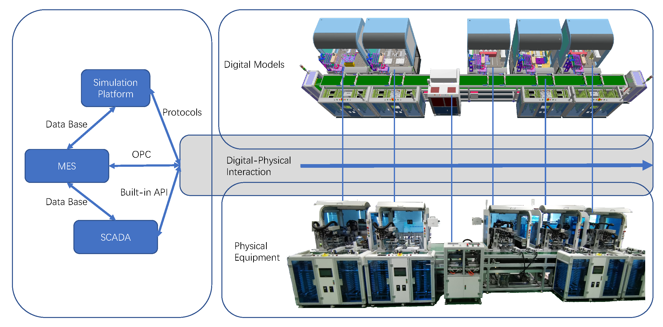
Three types of Digital Twins were introduced by Ghosh et al. [4]: (1) object twin, (2) process twin, and (3) phenomenon twin. The real-world manufacturing environment is collectively recreated in the cyber space, which is known as the object twin. To digitize the entire Digital Twin process from product design to manufacturing execution in physical space, realistic real-time digital models that reflect the physical system are essential to bridge the gap during the process [5], which concerns the synchronization between digital and physical entities. In the above context, computer-aided design (CAD) models driven by a Digital Twin are no longer simple time-independent three-dimensional (3D) objects hanging in empty space, but dynamic, precise, and complex representations [6] which form the basis for the Digital Twin capabilities. Such models not only serve the design verification and validation [7], but also are increasingly used as dynamic representations that include the model-based definition of the required product characteristics [8].

Nevertheless, over recent decades, advancements in computer technology have enabled the development of increasingly sophisticated virtual CAD models of physical artifacts [9]. These large-scale CAD models, which include processing equipment, storage, and transportation devices, as well as varying auxiliary devices, are generally involved in a Digital Twin-driven production line. Such customized CAD models are integrated with different-scale resolutions. Long rendering times turn into a technical barrier during a synchronizing process in a Digital Twin-driven production line. This barrier remains the same even under high-performance computing conditions. Data redundancy in 3D CAD models is a vital factor that affects synchronization. Consequently, lightweight 3D geometrical data have become necessary.

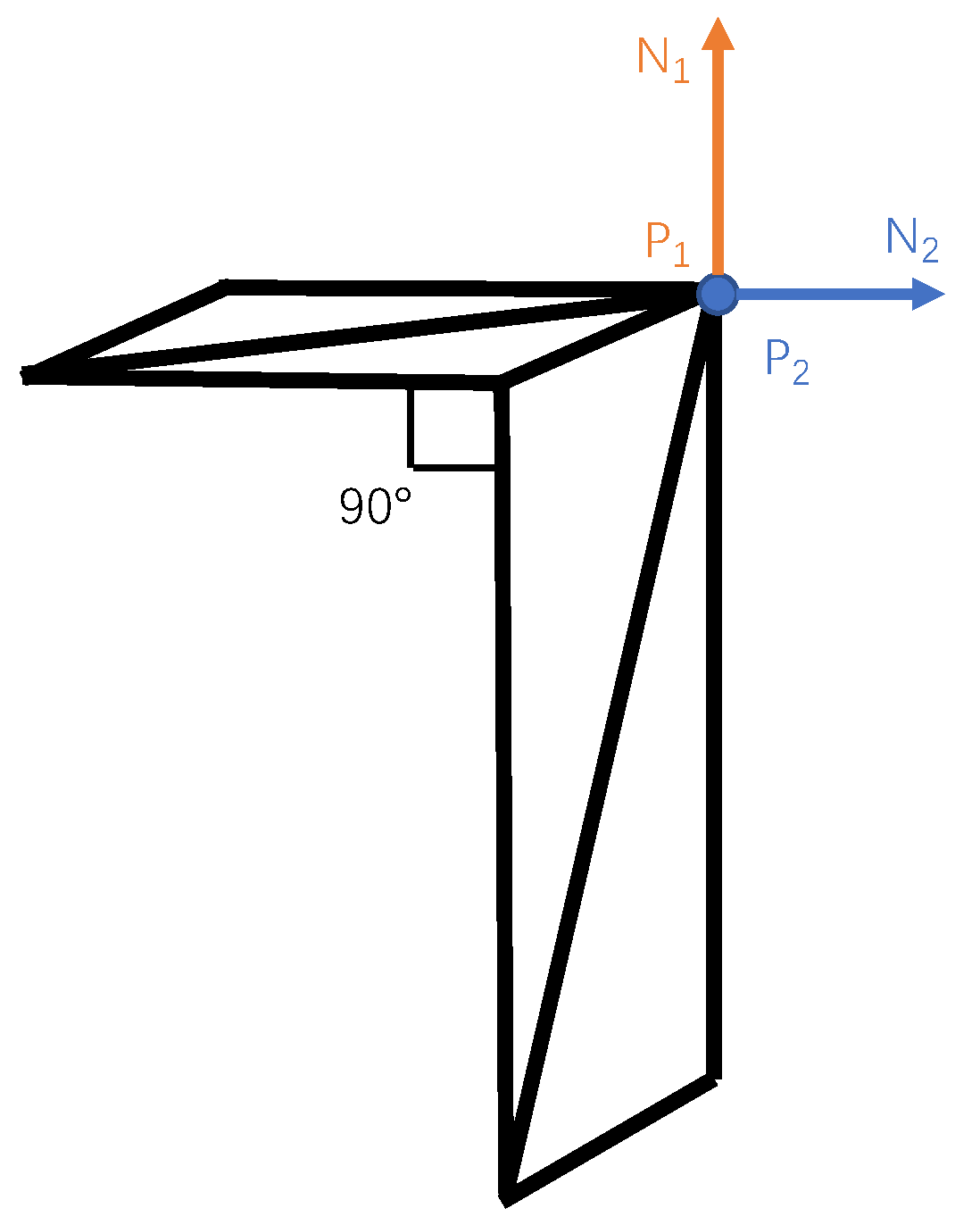
There is a conflict in achieving accurate synchronization while maintaining at the same time a high fidelity without losing useful feature information. To this end, an acceptable balance between these two factors should be found. However, various CAD models incorporated in Digital Twins are characterized by discrete folded corner planes, where two planes at the folded corners are repeatedly described by the edges and vertices that correspond to the two planes. As showed in Figure 1, the vertices $P_1$ and $P_2$ are repetitive, while the normal vectors $N_1$ and $N_2$ of the vertices are perpendicular to each other, to avoid the wrong information of plane normal vectors. Such CAD models often have extremely large volumes of geometrical data with complex data structures. When normal simplification algorithms are applied in the scenarios of Digital Twin-driven production lines, the surface breakage problem emerges, which leads to serious losses of significant features of the CAD model. Therefore, it is hard to preserve the real-time performance and high interaction accuracy between digital-physical entities. An effective lightweight mesh model approach is the top priority for performing feature-preserving operations of lightweight CAD models and preserve at the same time significant geometrical features.

In the scenarios of Digital Twin-driven production lines, CAD models can be divided into moving and non-moving parts. There are many negligible interfaces between the assemblies in the non-moving parts, which sacrifices a large amount of computer rendering performance. Thus, the lightweight approach is of great significance to keep the smooth motion coordination between digital and physical entities.

The rest of this paper is organized as follows: Section 2 briefly reviews the key related research streams in Digital Twins and mesh simplification; Section 3 presents a mesh simplification algorithm with several constraints and a penalty function; Section 4 describes the identification and simplification of interfaces based on interactive markers; in Section 5, the proposed algorithm steps are summarized; in Section 6, experimental results and analysis are demonstrated, and Section 7 draws the conclusions.

2. Related Works

The algorithm proposed in this study is based on Digital Twin technology, which is an effective solution to meet the demands for the design and operation of smart manufacturing systems. The concept of Digital Twin was first proposed and adopted by NASA for monitoring, safety, and reliability optimizations of spacecrafts [3]. The idea of the Digital Twin is to be able to design, test, manufacture, and use the virtual version of the systems [9], which includes more or less all information that could be useful in all the current and subsequent—lifecycle phases [10]. Digital Twins are applied in many different areas from many different perspectives [11,12], such as Product Lifecycle Management, Enterprise Resource Management, Supply Chain Management, cloud platforms including. analytics, diagnosis, etc. [13]. Different understandings of the Digital Twins can be observed in industrial practice [14]. Three types of Digital Twin were proposed by Ghosh et al. [4], which are object twin, process twin, and phenomenon twin, respectively. Here, an object twin means the Digital Twin of a real-world object used in a given manufacturing environment. A process twin means the Digital Twin of a process sequence in a given manufacturing environment. A phenomenon twin means the Digital Twin of a machining phenomenon in a given manufacturing environment. Digital Twin has bidirectional real-time connectivity with its physical counterpart. It has been stressed that Digital Twin needs semantically annotated content for fulfilling its bidirectional real-time connectivity. To construct the Digital Twin, five modules are needed. In addition, they can be listed as Input, Modeling, Simulation, Validation, and Output modules. In specific time-critical applications, the simulators are also expected to provide real-time information to the technology resulting in a hardware-in-the-loop (HIL) structure [15]. So, the HIL concept is usually used for real-time testing and validation of complex devices [16] and fault diagnosis in hardware development [17]. In the system management area [18], General Electric focuses on predicting the health and performance of their products over lifetime [19], while Siemens focuses on establishing a bridge between the digital model and the physical part [20]. In particular, more realistic and sophisticated virtual CAD models of manufactured products are essential to bridge the gap between design and manufacturing, as well as to couple real and virtual worlds [14].

The smart manufacturing system is often large in scale and complex in structure [21], which leads to the same scale and complexity of the CAD assembly digital models. Accordingly, large-scale CAD models have been generally involved in Digital Twin-driven production, which are supposed to be simplified to achieve a smooth interaction between digital and physical entities. Garland et al. [22] proposed a scheme of iterative edge contractions based on local Quadric Error Metrics (QEM). Their algorithm is capable of rapidly producing high-fidelity approximations of polygonal models. Nevertheless, it suffers from cumulative errors when dealing with large-scale models. In another study, Lindstrom et al. [23] calculated the projected distance from points to adjacent planes and took the area of the triangles as the constraint weight. Subsequently, the contraction target vertices were obtained from the square of the optimized volume. However, their algorithm has certain limitations in the terms of mesh quality and boundary influence. The same group [24] proposed an out-of-core mesh simplification algorithm, which extended the vertex clustering through error quadric information for the placement of the representative vertex of each cluster. Nevertheless, the manifold characteristics and topology of the original model could not be effectively preserved. Hoppe et al. [25] proposed a new QEM matrix with non-geometric attribute constraints, and by calculating the geometric distance norm and the attribute distance norm from a new vertex to any triangle, a fused quadratic matrix was obtained. This algorithm is effective in simplifying manifold CAD models, while there is still considerable room for improvement concerning detail feature preservation. Ho et al. [26] proposed a simplification algorithm where the user can select a specific area to retain the details; however, it has high user input requirements and is not easy to control.

In the past decade, simplification algorithms have become increasingly adaptive and effective. Ozaki et al. [27] proposed an external memory parallel computing framework for large-volume CAD models based on the classic QEM algorithm, using v-Supported Vector Machine (v-SVM) and the fuzzy C-means (FCM) clustering algorithm to classify regions. The data from different regions were processed through CPU/GPU, but the problem of losing detailed features was still not solved. To better control the detail preservation of local features, Jun et al. [28] introduced the concept of vertex curvature and added the corresponding curvature factor to QEM. However, only the normal vector of the vertex and the area of the adjacent triangles were taken into consideration. Consequently, their approach is suitable only for CAD models with relatively homogeneous mesh triangles. Liu et al. [29] proposed a lightweight algorithm with intelligent information reduction for large-scale CAD models, which can generate simplified CAD models using their intrinsic structures; still, user intervention is required, and certain components might be separated from the main body. Kwon et al. [30] used progressive control to remove sequentially the features acquired by volume decomposition. In this approach, the user intervenes in the progressive control stage and adjusts the Level of Details (LOD) for each component of the CAD assembly model; however, some geometric features cannot be recognized and thus cannot be simplified. Pellizzoni et al. [31] improved the QEM algorithm by enhancing the quadric error metrics with a penalizing factor based on discrete Gaussian curvature, which can be estimated efficiently through the Gauss-Bonnet theorem. During the edge decimation process, the presence of fine details is taken into consideration. Tariq et al. [32] used different vertex attributes in addition to geometry to simplify mesh instances with efficient time-space requirements and better visual quality; nevertheless, the impact of normals and textures was not taken into consideration.

In the simplification of CAD models of production equipment, the above-mentioned mesh simplification algorithms are prone to feature annihilation and uncontrolled errors. In particular, because the contraction cost in the algorithm is lower than the threshold, the features that need to be preserved in the subclass of models with fewer vertices and triangular facets can be contracted. Thus, unintended simplification results occur in the final simplified model, such as broken surfaces.

3. Mesh Simplification

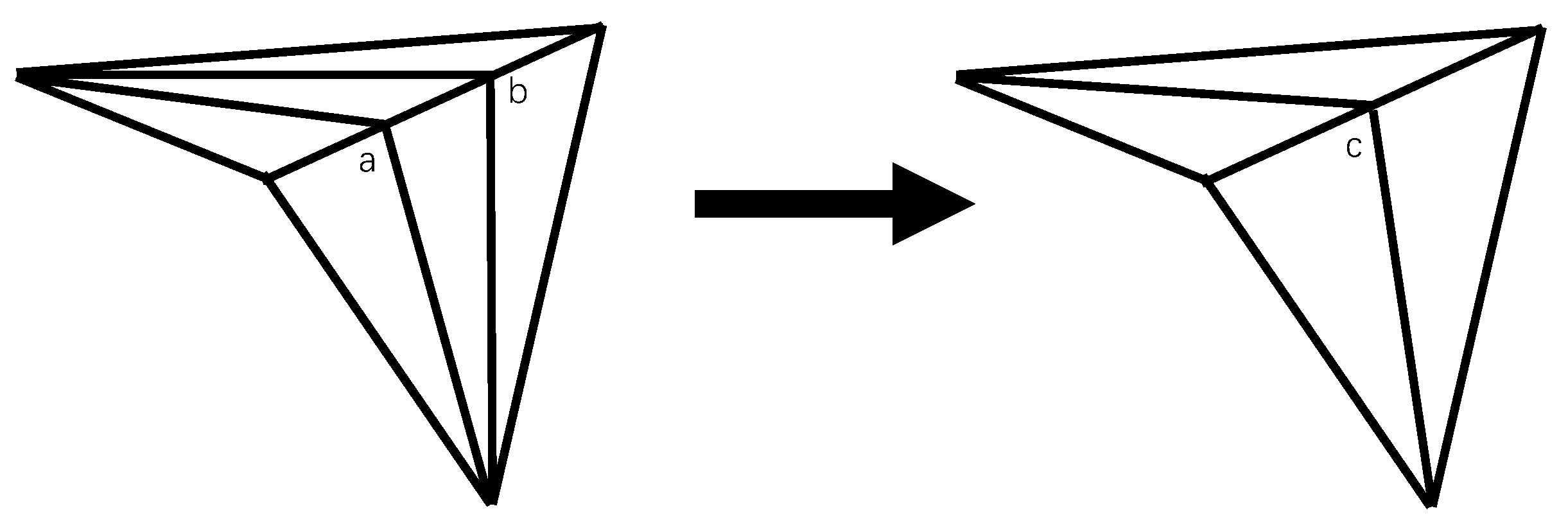
Realistic and sophisticated virtual CAD models of manufactured productions are essential to bridge the gap between design and manufacturing [14]. Thus, CAD models used in Digital Twins often have extremely large volumes of geometrical data with complex data structures. Such a model is the digital CAD model of a mobile phone production line with 33,310,548 vertices and 18,080,646 triangular facets [33], which requires mesh simplification using edge contractions, as shown in Figure 2, to obtain high-fidelity approximations of polygonal models for further operations. In this section, the repetitive mesh data are first pre-processed, and then, new constraints are introduced into the QEM matrix [22]. Finally, the optimal candidate contraction target is selected and the penalty function for narrow triangles is introduced.

To maintain the significant geometric features of CAD models and avoid any unexpected modifications during the simplification process, it is necessary to control the geometric error between the original CAD model and the simplified one. Common geometric error control approaches include Square Volume Measure [34], QEM [22], and Hausdorff distance Metrics [35]. Among them, QEM has the lowest time complexity, which can significantly improve the simplification efficiency. Therefore, in this paper, QEM is adopted to calculate the cost of each contraction target vertex.

3.1. Pre-Processing of Mesh Data

The correct normals should be stored in each plane for various assemblies in the Digital Twin. These models are composed of discrete folded corner planes, which are not similar to the ones composed of continuous planes that often appear in the aforementioned mesh simplification papers. To this end, it is necessary to pre-process the mesh data of common CAD assembly models. After all the non-repetitive vertex and edge objects are instanced, they are mapped to the mesh data one by one. Their unique hash codes are obtained by obfuscating the coordinate data of vertices and edges, and then, the repetitive vertices and edges are removed based on their hash codes.

$$H\left(v\right)=\sum \overrightarrow{p\left(v\right)}\times \overrightarrow{c}$$

(1)

where $H\left(v\right)$ is the hash value of each vertex; $\overrightarrow{p\left(v\right)}$ is the coordinate vector of each vertex, and $\overrightarrow{c}$ is the coefficient vector for obfuscation calculation.

Degenerate planes and edges are defined as the planes or edges that are decimated to a point. The degenerate planes and edges are removed, and the data structure abstraction operation of the entire mesh model is performed. Finally, the normal vector $\overrightarrow{n\left(f\right)}$ of each plane, as well as the distance d between the plane and the origin, are calculated.

$$\overrightarrow{n\left(f\right)}=\frac{\left(\overrightarrow{v_3}-\overrightarrow{v_1}\right)\times \left(\overrightarrow{v_2}-\overrightarrow{v_1}\right)}{\left|\left(\overrightarrow{v_3}-\overrightarrow{v_1}\right)\times \left(\overrightarrow{v_2}-\overrightarrow{v_1}\right)\right|}$$

(2)

$$d=\overrightarrow{n\left(f\right)}·\overrightarrow{v_1}$$

(3)

where $\overrightarrow{v_1},\overrightarrow{v_2},\overrightarrow{v_3}$ are the coordinate vectors of the three vertices on each triangular plane.

3.2. QEM

Subsequently, ${[x,y,z,1]}^T$ is defined as the certain vertex coordinate of the mesh model, and the plane equation of each triangle in it can be expressed by $ax+by+cz+d=0$, where $a^2+b^2+c^2=1$ and d is a constant. The error of an original vertex that contracts to a candidate contraction target vertex in the mesh is defined as the sum of the squares of distances to its first-order adjacent triangles:

$$\Delta \left(v\right)=\sum _{f\in NF\left(v\right)}{\left(C{o}_f^T{v}^{\prime }\right)}^2$$

(4)

where $C{o}_f={[a,b,c,d]}^T$ and $NF\left(v\right)$ represents the set of the first-order adjacent triangles of the original vertices. Thus, Equation (4) can be written as a quadratic expression:

$$\begin{array}{cc}\hfill \Delta \left(v\right)& =\sum _{f\in NF\left(v\right)}{v^{\prime }}^T\left(C{o}_{f}C{o}_f^T\right)v^{\prime }\hfill \\ \hfill & ={v^{\prime }}^T\left(\sum _{f\in NF\left(v\right)}C{o}_{f}C{o}_f^T\right)v^{\prime }\hfill \end{array}$$

(5)

where $Q\left(v\right)={\sum }_{f\in NF\left(v\right)}C{o}_{f}C{o}_f^T$, which is called the QEM matrix. Subsequently, the cost of an edge contracting to a candidate contraction target vertex can be determined by:

$$\begin{array}{cc}\hfill \Delta \left(v^{\prime }\right)& ={v^{\prime }}^{T}Q\left(v_1\right)v^{\prime }+{v^{\prime }}^{T}Q\left(v_2\right)v^{″}\hfill \\ \hfill & ={v^{\prime }}^T\left(Q\left(v_1\right)+Q\left(v_2\right)\right)v^{\prime }\hfill \end{array}$$

(6)

where $Q\left(v_1\right),Q\left(v_2\right)$ are the QEM matrices of two vertices on the contracted edge. Therefore, in this section, all vertices of the mesh model are traversed and the corresponding $Q\left(v\right)$ is calculated.

3.3. Connection Properties and Discrete Folded Corner Constraints

By calculating the dihedral angle of adjacent faces, the local connection properties (concave or convex) can be obtained, which restrains the folded corner edge of the CAD model from being simplified. By acquiring the information of the adjacent triangles of each edge, the edges on the boundary are ignored. The centroid coordinates $\overrightarrow{v_{10}}(x_{10},y_{10},z_{10}),\overrightarrow{v_{20}}(x_{20},y_{20},z_{20})$ and the normal vectors $\overrightarrow{n_1},\overrightarrow{n_2}$ corresponding to the qualified adjacent triangles can be calculated as follows:

$$\left\{\begin{array}{c}{x}_0=\left(x_1+x_2+x_3\right)/3\hfill \\ y_0=\left(y_1+y_2+y_3\right)/3\hfill \\ z_0=\left(z_1+z_2+z_3\right)/3\hfill \end{array}\right.$$

(7)

where $x_i,y_i,z_i$ are the coordinates of the three vertices of a triangle.

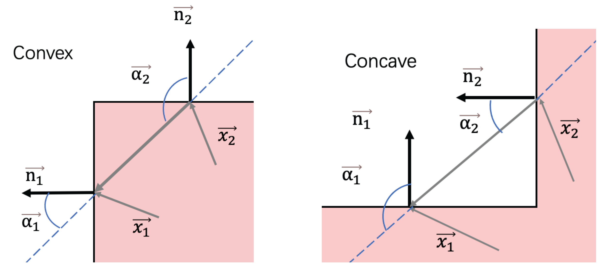
As shown in Figure 3, based on the relationship between the normal vector of adjacent triangles and the one connecting their centroids, it can be determined whether the connection property between the adjacent triangles is convex or concave. After the vector between the centroids $\overrightarrow{d}$ and the normal vectors $\overrightarrow{n_1},\overrightarrow{n_2}$ have been normalized, the connection property between the adjacent triangles is convex (or vice versa) if:

$$\begin{array}{cc}\hfill {\alpha }_1<{\alpha }_2& \Rightarrow cos\left({\alpha }_1\right)-cos\left({\alpha }_2\right)<0\hfill \\ \hfill & \iff \overrightarrow{{\mathrm{n}}_1}·\overrightarrow{d}-\overrightarrow{{\mathrm{n}}_2}·\overrightarrow{d}<0\hfill \end{array}$$

(8)

To avoid the precision noise, a deviation is introduced to deal with the approximately vertical connection properties.

$$\begin{array}{cc}\hfill \beta & =\left|\angle \left(\overrightarrow{n_1},\overrightarrow{n_2}\right)-\frac{\pi }{2}\right|\hfill \\ \hfill & =\left|{cos}^{-1}\left(\overrightarrow{n_1}·\overrightarrow{n_2}\right)-\frac{\pi }{2}\right|<{\beta }_{\mathrm{Thres}}\hfill \end{array}$$

(9)

If the deviation meets the threshold given as Equation (9), the dihedral angle of the adjacent triangles is introduced into the QEM matrix as an adaptive weight. In addition, corresponding positive and negative quantities are assigned according to their connection properties.

$$Q\left(v\right)=Q\left(v\right)\times \angle \left(\overrightarrow{n_1},\overrightarrow{n_2}\right)$$

(10)

3.4. Plane Geometric Constraints

The normal vector of each plane $\overrightarrow{n}$ and the distance d between plane and origin are used to generate the corresponding $Q\left(v\right)$ matrix.

$$Q\left(v\right)=Q\left(v\right)+\left[\begin{array}{c}\overrightarrow{n}\hfill \\ d\hfill \end{array}\right]\times \left[\begin{array}{cc}\overrightarrow{n}\hfill & d\hfill \end{array}\right]$$

(11)

Then, $Q\left(v\right)$ is multiplied by the triangular patch area, which is introduced as a triangular patch weight to the constraint:

$$\begin{array}{cc}\hfill Q\left(v\right)& =Q\left(v\right)\times S\left(f\right)\hfill \\ \hfill & =Q\left(v\right)\times \frac{\left(\overrightarrow{v_2}-\overrightarrow{v_1}\right)\times \left(\overrightarrow{v_3}-\overrightarrow{v_1}\right)}{2}\hfill \end{array}$$

(12)

where $\overrightarrow{v_1},\overrightarrow{v_2},\overrightarrow{v_3}$ denote the coordinates of the three vertices of the triangle.

3.5. Boundary Constraints

The edge is defined as “boundary”; that is, the edge has discontinuity if the number of adjacent triangles is equal to 1. First, the continuity of the edge is checked, then, all the edges are traversed, the matrix of discontinuous constraints (boundary constraints) is calculated and added to the matrix $Q\left(v\right)$, and finally, a triangular patch weight is introduced.

$$\overrightarrow{n_2}=\overrightarrow{e}\times \overrightarrow{n_{neigh}}=\left(\overrightarrow{v_2}-\overrightarrow{v_1}\right)\times \overrightarrow{n_{neigh}}$$

(13)

$$d=-\overrightarrow{n_1}·\overrightarrow{v_2}$$

(14)

$$Q\left(v\right)=Q\left(v\right)+\left[\begin{array}{c}{\overrightarrow{n}}_2\hfill \\ d\hfill \end{array}\right]·\left[\begin{array}{cc}{\overrightarrow{n}}_2\hfill & d\hfill \end{array}\right]$$

(15)

where $\overrightarrow{n_2}$ is the vector parallel to the plane of the calculated edge, $\overrightarrow{e}$ is the vector between two vertices of the edge, ${\overrightarrow{n}}_{neigh}$ is one of the normal vectors of first-order adjacent triangles of the calculated edge, $\overrightarrow{v_1},\overrightarrow{v_2}$ are the vertices of the calculated edge, and d is the distance between the calculated edge and the origin of coordinates.

3.6. Optimal Candidate Contraction Target

By traversing all the edges in the CAD model, the candidate contraction target vertex is iteratively selected, and the corresponding contraction c is calculated. Finally, the edges are pushed into the stack and stored in order from small to large.

$$\begin{array}{cc}\hfill c& =\Delta \left(v^{\prime }\right)={v^{\prime }}^{T}Q\left(v_1\right)v^{\prime }+{v^{\prime }}^{T}Q\left(v_2\right)v^{\prime }\hfill \\ \hfill & ={v^{\prime }}^T\left(Q\left(v_1\right)+Q\left(v_2\right)\right)v^{\prime }\hfill \end{array}$$

(16)

Due to the fact that the significant features of CAD models in Digital Twins should be preserved as much as possible, the possibility of significant features being modified should be reduced. To this end, the contraction target selection process is constrained to the dimensions of each edge that is about to be contracted. According to Equation (16), the contraction cost of the edge composed of $\overrightarrow{v_1}$ and $\overrightarrow{v_2}$ to a contraction target vertex $\overrightarrow{v^{\prime }}$ is as follows:

$$\Delta \left({\overrightarrow{v}}^{\prime }\right)={\overrightarrow{v}}^{\prime T}Q{\overrightarrow{v}}^{\prime }$$

(17)

$${\overrightarrow{v}}^{\prime }=\overrightarrow{v_2}+a·\overrightarrow{d}$$

(18)

$$\overrightarrow{d}=\overrightarrow{v_1}-\overrightarrow{v_2}$$

(19)

In Equation (18), a represents the relative offset coefficient of the contraction target vertex on the edge. The following equation can be obtained by substituting Equation (18) into Equation (17), and performing polynomial transformation:

$$\begin{array}{cc}\hfill & \Delta \left({\overrightarrow{v}}^{\prime }\right)={\left(\overrightarrow{v_2}+a·\overrightarrow{d}\right)}^{T}Q\left(\overrightarrow{v_2}+a·\overrightarrow{d}\right)\hfill \\ \hfill & ={\overrightarrow{d}}^{T}Q\overrightarrow{d}·a^2+\left({\overrightarrow{v}}_2^{T}Q\overrightarrow{d}+{\overrightarrow{d}}^{T}Q\overrightarrow{v_2}\right)·a+{\overrightarrow{v_2}}^{T}Q\overrightarrow{v_2}\hfill \end{array}$$

(20)

Since a is an unknown variable, Equation (20) can be regarded as a univariate quadratic function. According to the function properties, a minimum value exists in the expression, and the derivative of the expression can be obtained as follows:

$$2·{\overrightarrow{d}}^{T}Q\overrightarrow{d}·a+{\overrightarrow{v_2}}^{T}Q\overrightarrow{d}+{\overrightarrow{d}}^{T}Q\overrightarrow{v_2}=0$$

(21)

After the polynomial transformation of Equations (21) and (22) can be obtained:

$$a=\frac{{\overrightarrow{v_2}}^{T}Q\overrightarrow{d}+{\overrightarrow{d}}^{T}Q\overrightarrow{v_2}}{2·{\overrightarrow{d}}^{T}Q\overrightarrow{d}}$$

(22)

Consequently, the coordinate of the contraction target vertex can be calculated by substituting Equation (22) into Equation (18).

3.7. Penalty Function Design for Narrow Triangles

In some special cases, narrow triangles exist in the simplified mesh model, which can lead to unexpected irregularities. Currently, the regularity of a triangle is often used to determine whether a triangle is narrow, and the so-called regularity refers to the degree to which the triangle approaches an equilateral one. The equation reported in [28] is used to calculate the regularity of the triangles after CAD model simplification, while the regularity is used as a penalty function to correct the coordinate of the candidate contraction target vertex. The regularity can be calculated as:

$$r=\left(4\sqrt{3}A\right)/\left(l_1^2+l_2^2+l_3^2\right)$$

(23)

where A represents the area of the triangle, $l_1,l_2,l_3$ are the lengths of the three sides of the triangle, and r describes the regularity of the triangle. The more approximate the r is to 1, the better the quality of the triangle ($r=1$: equilateral triangle; $r\approx 0$: extremely narrow triangle).

4. Identification and Simplification of Interfaces

After simplifying the CAD model, the mesh model undergoes mesh segmentation. Each flat plane region in the triangular mesh model, as well as the corresponding vertices on the boundaries of the region, is identified.

Subsequently, the watershed segmentation algorithm [36] is employed to segment the mesh model, which identifies the plane regions and the boundaries of these regions based on the discrete curvature of the vertices. Afterward, the region clustering method is used to post-process the segmentation results; that is, region merging is performed to avoid the problem of over-segmentation.

4.1. Mesh Segmentation and Region Identification

The Voronoi area [37] is used to calculate the average curvature $K_H\left(\overrightarrow{v_i}\right)$ of the first-order adjacent triangle of each vertex $\overrightarrow{v_i}$, and the calculation equation is as follows:

$$\begin{array}{c}\hfill K_H\left(\overrightarrow{v_i}\right)=\frac{1}{4A_{mix}}\sum _{j\in N\left(i\right)}\left(cot{\phi }_{ij}+cot{\psi }_{ij}\right)\left({\overrightarrow{v}}_i-{\overrightarrow{v}}_J\right)·\overrightarrow{n}\end{array}$$

(24)

where $\overrightarrow{n}$ is the normal vector of each triangle, $\overrightarrow{v_j}$ is one of the adjacent vertices of the vertex $\overrightarrow{v_i}$, ${\phi }_k$ and ${\psi }_k$ are the diagonals of the edge where $\overrightarrow{v_i},\overrightarrow{v_j}$ are located; $A_{mix}$ is the sum of the areas $S_{v_i}$ of the first-order adjacent triangles of the vertex $\overrightarrow{v_i}$, which can be calculated as follows:

$$A_{mix}=\sum _i{S}_{v_i}$$

(25)

According to the Gauss-Bonnet theorem in differential geometry [38], the Gaussian curvature $K_G\left(\overrightarrow{v_i}\right)$ of each vertex $\overrightarrow{v_i}$ can be calculated by:

$$K_G\left({\overrightarrow{v}}_l\right)=\frac{1}{A_{mix}}\left(2\pi -\sum _{j\in N\left(i\right)}{\theta }_k\right)$$

(26)

where ${\theta }_k$ denotes the angle between the vertex $\overrightarrow{v_i}$ and the k-th triangle surface in its first-order neighborhood, and $A_{mix}$ denotes the sum of the areas of the first-order adjacent triangles of the vertex $\overrightarrow{v_i}$. Finally, the discrete curvature of the mesh vertices can be determined through the average and Gaussian curvature:

$$K\left(v_i\right)=K_H\left(v_i\right)-\sqrt{K_H^2\left(v_i\right)-K_G\left(v_i\right)}$$

(27)

After the discrete vertex curvatures have been calculated, the vertices with the minimum local curvature are identified, and then, the segmented region of all the other mesh elements is determined by the multi-directional gradient descent search. Subsequently, the algorithm searches for vertices whose curvature value is lower than that of all other adjacent vertices, and any local minimum vertices are marked out.

According to this, the flat region is iteratively marked, then, the vertices with the smallest and uneven local curvature are marked, and finally, the mesh vertices which are flat relative to these vertices are marked to achieve the initialization minimum. If the vertex has two region segmentation markers, the mesh vertex is marked as a boundary vertex.

Finally, region clustering is used to merge the segmented regions and update the boundary marks of the mesh vertices.

4.2. Identification and Designation of Interfaces Based on Interactive Markers

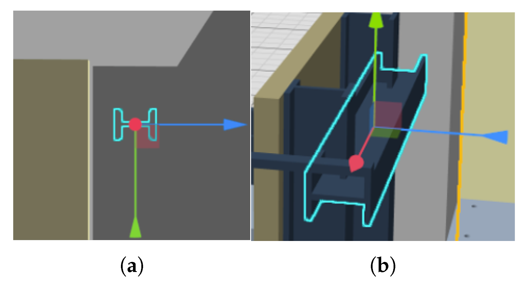
There are often many interfaces between parts of CAD assembly models. These interfaces often exist in the gaps of the CAD model parts, which cannot be observed by users during the operation of Digital Twins. For CAD assembly models that belong to the non-moving parts, these interfaces have no effect on the running process and solution results.

Consequently, rendering these contents in the simulation engine is a waste of computer performance. Thus, they can be simplified and removed to further reduce the cost of the computer rendering process.

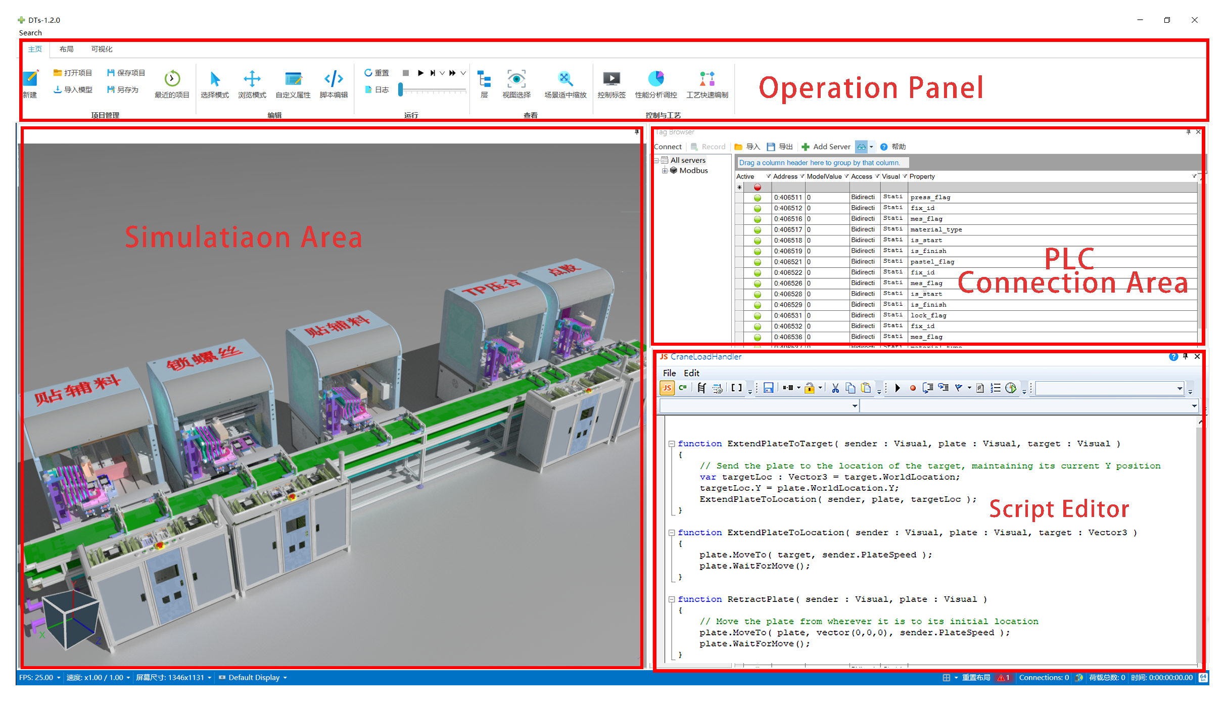
A self-developed Digital Twin system is used, and a contour recognition scheme is added to the UI, as shown in Figure 4, which is used to highlight the interfaces.

In the next step, the approach of Metro [39] is used to evaluate the proximity between two planes based on the approximate distance. According to coordinates of vertices on the boundaries marked after segmentation, the seed point $\overrightarrow{p}$ of the segmented plane can be selected, and then, the Euclidean geometric distance between the vertex $\overrightarrow{p}$ and another segmented plane S can be calculated:

$$e(\overrightarrow{p},S)=\underset{p^{\prime }\in S}{min}d\left(p,p^{\prime }\right)$$

(28)

where $p^{\prime }$ is any point in the plane S and $d(p,p^{\prime })$ is the Euclidean geometric distance between p and $p^{\prime }$. The unilateral distance between the two segmented planes $S_1$ and $S_2$ can be defined as:

$$E\left(S_1,S_2\right)=\underset{p\in S_1}{min}e\left(p,S_2\right)<E_{Thres}$$

(29)

where $E_{Thres}$ is the Euclidean geometric distance threshold set by the user to determine whether the distance between the planes is close.

The segmented planes whose geometric distance is less than the threshold $E_{Thres}$ are removed, and they are highlighted on the UI for interface identification. Finally, it is provided by the user interaction to determine whether the interfaces need to be simplified.

5. Algorithm Description

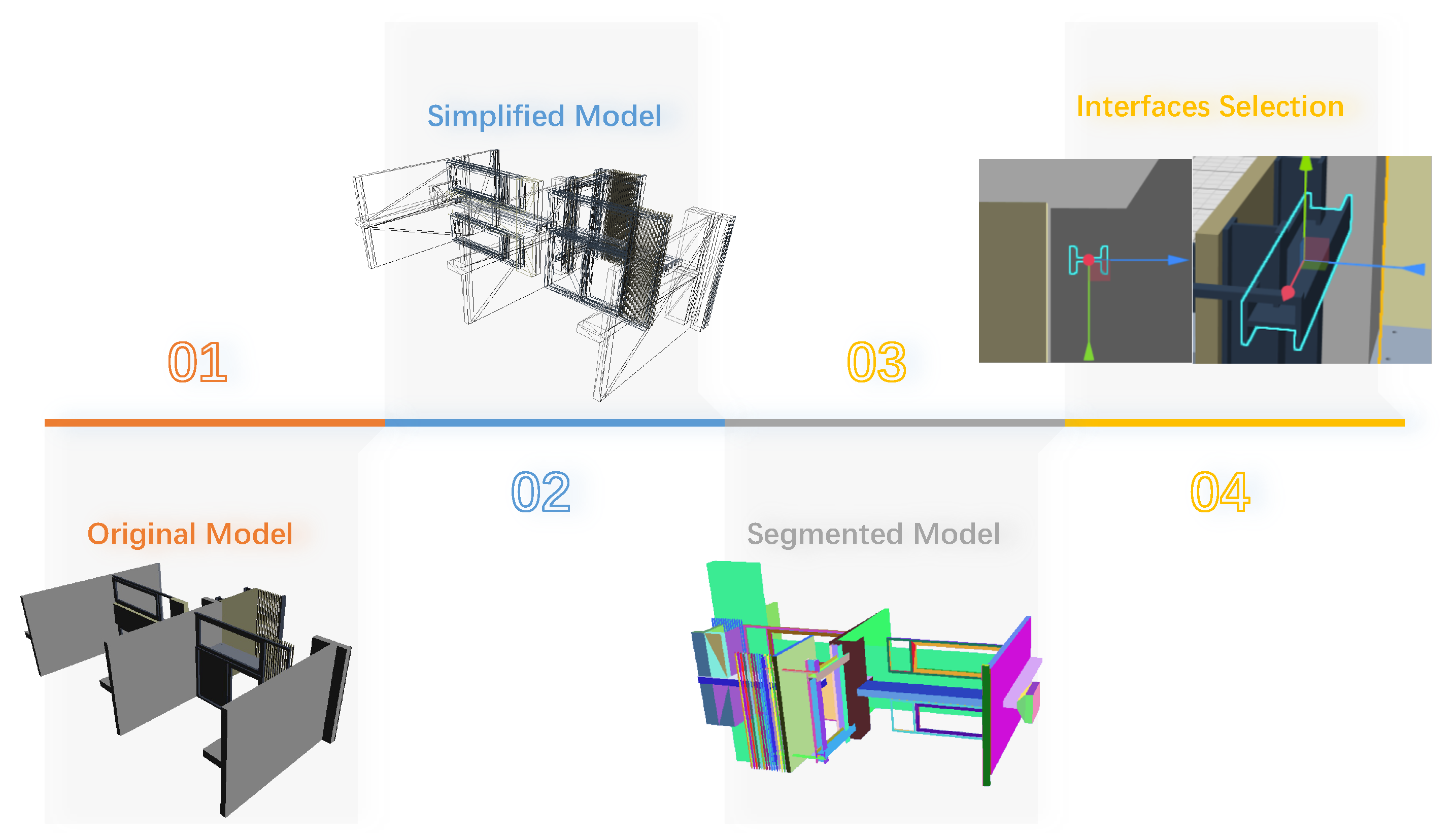
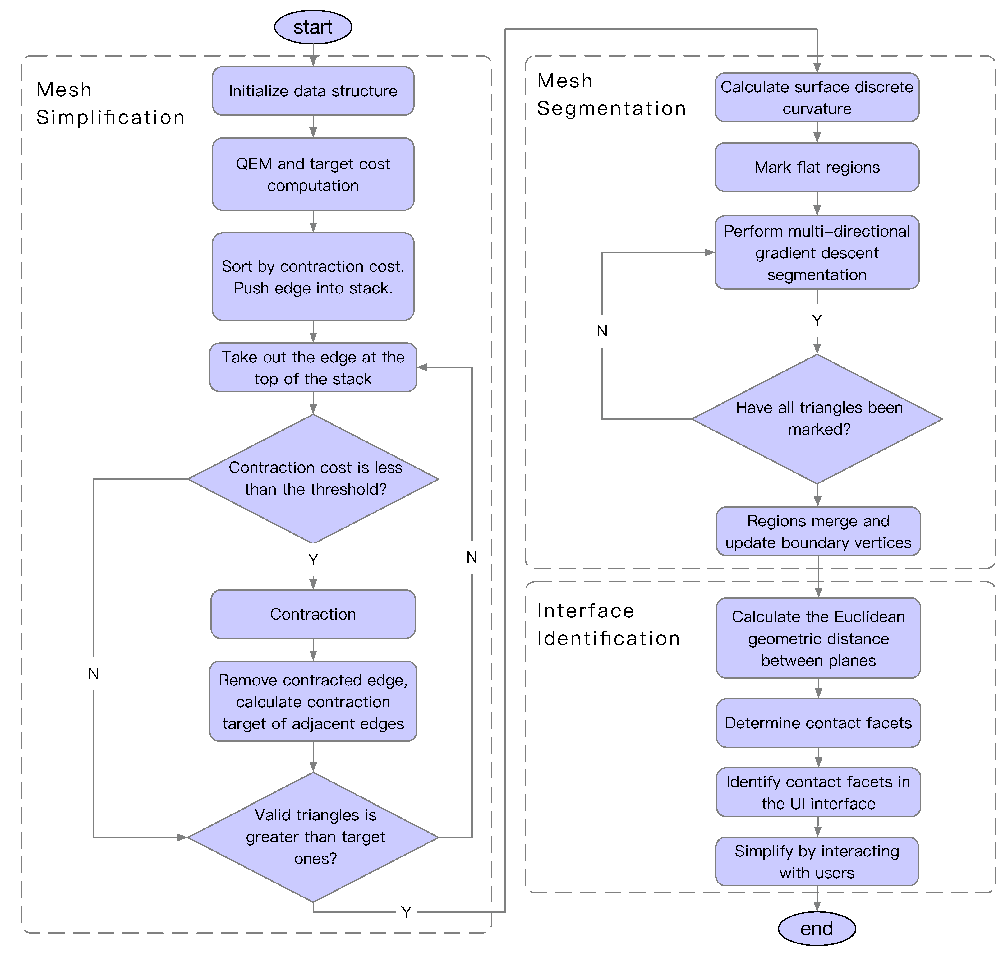
In this paper, an adaptive lightweight algorithm of mesh models is proposed, which is suitable for the simplification of sophisticated CAD assembly models of common production lines in Digital Twins. The output effects of each stage are shown in Figure 5. The specific process is exhibited in Figure 6. The steps of the proposed algorithm are summarized as follows:

Step 1. The vertices, normals, and indices are fetched from the CAD model file; then, they are saved to describe the topological structure of the mesh model;

Step 2. Discrete folded corner constraints, mesh boundary constraints, and plane geometric constraints are introduced; then, the QEM matrices for each vertex are generated;

Step 3. The candidate contraction target vertices of the edges in the mesh model are traversed one by one. Subsequently, the edge contraction cost is calculated based on the vertex, and the contraction cost is corrected by the triangle regularity penalty function. Finally, the edge objects are pushed into the contraction cost stack in the order from the smallest to the largest cost;

Step 4. The mesh simplification operations are executed iteratively. Each operation pops out the edge from the top of the stack and the edge contraction operation is performed. The contraction costs of the adjacent edges of the contracted edge and the optimal contraction target vertices are traversed and calculated, and the cost stack is updated. If the number of effective triangles is lower than or equal to that of the target ones, or the minimum cost of edges is lower than or equal to the error threshold, the edge contraction is stopped;

Step 5. The simplified mesh models are generated;

Step 6. The discrete surface curvatures of the vertices are traversed and calculated;

Step 7. The mesh vertices with the smallest local curvature are pushed into the stack with the smallest local curvature;

Step 8. The multi-directional gradient descent search is employed to traverse the segmentation area information of the mesh elements. If the vertices with a curvature value lower than that of all the adjacent vertices are local minimum vertices, the local minimum vertices are marked as flat regions and are pushed into the flat region stack;

Step 9. The mesh vertices with the smallest local curvature and those that are flat relative to them are marked for segmentation; then, the minimum surface discrete curvature is initialized;

Step 10. The remaining unmarked mesh vertices can be marked based on the tags of the marked mesh vertices;

Step 11. If the mesh vertex has two region tags, the mesh vertex will be marked as a boundary vertex;

Step 12. The segmented regions are merged through region clustering, and the boundary markers of the mesh vertices are updated;

Step 13. The Euclidean geometric distance between segmented planes is calculated. If the distance is less than the threshold distance set by the user, it is considered that the topological relationship between the two planes may be that of contact; where these two planes are defined as the interfaces;

Step 14. The interfaces are identified and highlighted on the UI, and ultimately it is up to the user to determine whether these interfaces should be simplified. In the end, the final lightweight mesh model is generated.

6. Results

6.1. Comparative Data Analysis

In this section, experiments were performed using IntelliJ IDEA and the self-developed Digital Twin system (DTs). All experiments were conducted on a commodity PC with Intel Core i7 3.6 GHz and 8 GB 2400 MHz DDR3 RAM.

In this experiment, the lightweight mesh models were common CAD assembly models, including a shelf model, a robot base model, and a stereoscopic warehouse model. Figure 7, Figure 8 and Figure 9 illustrate the visual quality of the lightweight mesh models generated using different algorithms.

In this paper, the Hausdorff distance [35] was used to compare the geometric errors of the CAD models before and after simplification, to evaluate the effect of each algorithm on the visual quality of the CAD models. The examples compared in this paper are common CAD assembly models with complex topologies, i.e., shelf model, robot base model, and stereoscopic warehouse model. Figure 7, Figure 8 and Figure 9 are the visual quality results of the above models obtained by different algorithms; (a) shows the original mesh model; (b)∼(d) present respectively the results of the QEM [22], Huang et al. [28], and proposed algorithms after a triangle number reduction to 80%; and (e)∼(g) are models simplified to 40%; and (h)∼(j) are models simplified to 20%.

As it can be observed in the above figures, the ability of the proposed algorithm to retain the significant geometric features of common CAD assembly models with complex topology was significantly stronger than that of the QEM [22] and Huang’s [28] algorithms. When the CAD models were simplified to 80%, 40% and 20% respectively using QEM [22], some significant features of the lightweight CAD models were lost, and serious breakage occurred. Although the detailed features of the lightweight CAD models generated by the algorithm of Huang et al. [28] were partially preserved, there were still some broken surfaces.

On the other hand, the contour features of the lightweight mesh model generated by the proposed algorithm were still clear and identifiable, the detailed features were also maintained well, and there were no broken surfaces. According to

Table 1. Comparison of the simplification errors of the shelf models simplified by the different algorithms to different proportions.

Proportion	Algorithm	Max Error	Average Error	Mean Square Error
	QEM	100.717	7.0282	14.1726
60%	Approach of [28]	7.2968	0.17084	0.65437
	Proposed Approach	0.00495	3 $\times {10}^{-5}$	9.7 $\times {10}^{-5}$
	QEM	100.717	3.93728	10.6638
40%	Approach of [28]	4.7807	0.09281	0.43418
	Proposed Approach	0.00443	1 $\times {10}^{-6}$	4.5 $\times {10}^{-5}$
	QEM	42.3065	1.57891	4.23958
20%	Approach of [28]	2.62158	0.00898	0.13053
	Proposed Approach	0.005	2 $\times {10}^{-6}$	5.2 $\times {10}^{-5}$

,

Table 2. Comparison of the simplification errors of the robot base models simplified by the different algorithms to different proportion.

Proportion	Algorithm	Max Error	Average Error	Mean Square Error
	QEM	0.1235	0.00392	0.0167
60%	Approach of [28]	0.02756	0.001842	0.00559
	Proposed Approach	0.00494	2 $\times {10}^{-6}$	9.7 $\times {10}^{-5}$
	QEM	0.1235	0.00287	0.01443
40%	Approach of [28]	0.02744	1.2 $\times {10}^{-3}$	3.7 $\times {10}^{-3}$
	Proposed Approach	0.00443	1 $\times {10}^{-6}$	4.5 $\times {10}^{-5}$
	QEM	0.1235	0.002565	0.01331
20%	Approach of [28]	4.3 $\times {10}^{-3}$	2.8 $\times {10}^{-5}$	2.4 $\times {10}^{-4}$
	Proposed Approach	0.005	2 $\times {10}^{-6}$	5.2 $\times {10}^{-5}$

and

Table 3. Comparison of the simplification errors of the stereoscopic warehouse models simplified by the different algorithms to different proportions.

Proportion	Algorithm	Max Error	Average Error	Mean Square Error
	QEM	1.48279	0.46217	0.67795
60%	Approach of [28]	4.4 $\times {10}^{-3}$	3.7 $\times {10}^{-4}$	1.2 $\times {10}^{-3}$
	Proposed Approach	0.00236	0.00038	0.00727
	QEM	0.96475	0.15869	0.27065
40%	Approach of [28]	0.01	2.7 $\times {10}^{-4}$	1.4 $\times {10}^{-3}$
	Proposed Approach	0.00063	0.00004	9.8 $\times {10}^{-5}$
	QEM	0.61697	0.07166	0.16939
20%	Approach of [28]	7.3 $\times {10}^{-3}$	9.7 $\times {10}^{-5}$	7.8 $\times {10}^{-4}$
	Proposed Approach	9.2 $\times {10}^{-5}$	1 $\times {10}^{-6}$	1.6 $\times {10}^{-5}$

, the geometric errors of the shelf and stereoscopic warehouse models simplified by the proposed algorithm were relatively smaller than those generated by the QEM [22] and Huang et al. [28] algorithms. Since the robot base model is similar to common continuous plane mesh models, the geometric errors of the proposed algorithm were similar to those of Huang et al. Consequently, the geometric errors of the proposed algorithm were not much different from those of Huang et al. [28], but were still much smaller than those of QEM [22].

6.2. Running Results of Digital Twins

Figure 10 shows the logical structure of the Digital Twin process. The key to Digital Twins lies in the real-time performance and accurate data synchronization in the interaction of digital-physical entities. The real-time data synchronization between the on-site physical equipment and the digital simulation CAD model is achieved by embedding the objects controlled by the Digital Twin process into online databases, industrial Ethernet protocols, and built-in application programming interfaces. Finally, it is presented in a synchronized manner with multiple views (Simulation View, Monitoring View, Execution View, and Physical View). On the one hand, by realizing the interaction of digital-physical entities between the Manufacturing Execution System (MES), the on-site physical equipment, and the simulation CAD model, it turns the original Sequential design into a parallel design. On the other hand, the system performance can be quickly and remotely tested through distributed hardware-in-the-loop testing to avoid full-line on-site testing [40].

In the above process, the real-time performance and accuracy of data transmission are self-evident, and a lightweight approach is urgently needed to provide strong support for it.

The DTs mentioned in this study support rapid customization of the workshop, production simulation, distributed integration and virtual debugging, performance control optimization, etc. It couples with 3D modeling, semi-physical simulation, and multi-view Functional modules such as synchronization (Digital Twin), virtual and real mutual control, and performance analysis.

In this study, a complete Digital Twin scenario of the entire mobile phone production line was built (Figure 11) based on DTs, and its running frame rate was recorded. All experiments were conducted on a commodity PC with Intel Core i7 3.6 GHz and 8 GB 2400 MHz DDR3 RAM.

The digital CAD models of the mobile phone production line equipment shown in Figure 12 had a huge amount of data with 33,310,548 vertices and 18,080,646 triangular facets. If the CAD model were imported directly into the Digital Twin software for further operation, it would introduce a huge challenge to the rendering performance of the computer, and the user would perceive an operation lag. Therefore, the real-time performance and accuracy of its life cycle data would not be guaranteed.

In Figure 13 and Figure 14, it is apparent that the application of the proposed lightweight algorithm resulted in an increase of average frame rate and a smoother frame rate fluctuation. The proposed lightweight algorithm improved tremendously the user experience. The average frame rates before and after the lightweight operation were 34.15 fps and 48.22 fps, respectively.

For a complete Digital Twin scene of the entire mobile phone production line, the experimental results demonstrated that the proposed lightweight algorithm can effectively improve the frame rate and stabilize the frame rate performance.

7. Conclusions

In this paper, a mesh segmentation algorithm is integrated into the mesh simplification algorithm, and the mesh discrete folded corner edge constraint and triangle regularity are introduced. The invisible interfaces between the assemblies are recognized and simplified. A lightweight approach that is applicable to various types of complex CAD assembly models of the production line equipment in Digital Twins has been proposed. The experimental results revealed that the geometric errors are reduced, and the running frame rates are relatively improved, while the significant and detailed features of the original mesh model are maintained with high quality. A high-quality 3D mesh digital CAD model for Digital Twins is obtained, which can strongly support the accuracy and efficiency of the interaction between digital and physical entities.