Article

On the Design of a Class of Rotary Compressors Using Bayesian Optimization

School of Engineering, IT and Physical Sciences, Federation University Australia, Mount Helen, Ballarat, VIC 3353, Australia
*
Author to whom correspondence should be addressed.
Machines 2021, 9(10), 219; https://doi.org/10.3390/machines9100219
Submission received: 16 August 2021 / Revised: 22 September 2021 / Accepted: 27 September 2021 / Published: 29 September 2021
(This article belongs to the Special Issue Advances in Positive Displacement Compressors)

Abstract

:
The optimization process of compressors is usually regarded as a ‘black-box’ problem, in which the mathematical form underlying the relationship between design parameters and the design objective is impractical and costly to be obtained. To solve the ‘black-box’ problem, Bayesian optimization has been proven as an accurate and efficient method. However, the application of such a method in the design of compressors is rarely discussed, particularly no work has been reported in terms of the positive displacement type compressor. Therefore, this paper aims to introduce the Bayesian optimization to the design of positive displacement compressors through the optimization process of the novel limaçon compressor. In this paper, a two-stage optimization process is presented, in which the first stage optimizes the geometric parameters as per design requirements and the second stage focuses on revealing an optimum setting of port geometries that improves machine performance. A numerical illustration is offered to prove the validity of the presented approach.

1. Introduction

In compressor design, information solely obtained from the simulation of the mathematical model is usually insufficient to reflect the thorough relationship between the design parameters and design objective in terms of performance. As such, designers often need to rely on optimization strategies to reveal the optimum design scenario before reaching the final decision on the prototype.
The published literature shows that various optimization techniques have been applied to the design optimization of the positive displacement machine and compressor in particular. Ooi [1] applied the direct-search method to seek a set of six machine dimensions and seven design constraints, which can minimize the mechanical losses of the rolling piston compressor. The author reported that a predicted 50% reduction in mechanical loss, which increases 14% of the coefficient of performance, can be achieved with a proper combination of design dimensions. Liu et al. [2] employed the gradient search method to determine optimum dimensions of bearing components that can reduce the frictional loss occurring in the scroll compressor. Based on the optimization result, the author found that the frictional loss can be reduced in the range of 14.1% to 18.1%. Sultan and Kalim [3] adopted the simultaneous perturbation stochastic approximation (SPSA) method to find the best piston trajectory of the reciprocating compressor, and the authors also employed the gradient-based optimization to determine the machine dimensions which can realize such a trajectory. Recently, the SPSA approach has also been utilized in the work of Phung and Sultan [4] to design a new embodiment of the limaçon machine referred to as the limaçon-to-circular machine. Like other limaçon machine embodiments, this new design can be used as expanders, compressors, and potentially pumps. Cavazzini et al. [5] adopted topology optimization, which combines the particle swarm method with the computational fluid dynamics, to determine the geometric parameters that can maximize the machine efficiency of the scroll compressor. The authors discovered that the compressor performance is more sensitive to the variation of three parameters, which are the size of the discharge port, the number of coils, and the radius of orbiting scroll. Silva and Dutra [6] used the genetic optimization algorithm to find an optimum piston trajectory that maximizes the performance of the reciprocating compressor. The authors reported that the optimum piston trajectory reduces the losses from the heat transfer and leakage, increasing the thermodynamic efficiency from 88.3% to 92.1% and the volumetric efficiency from 70.9% to 72%. In their latest work, Aw and Ooi [7] presented a comprehensive review of the previous investigation conducted on sliding-vane and rolling piston compressors. The authors discussed various aspects of these two types of compressors and pointed out the importance of the optimization process with respect to the development and design evolution of rotary type compressors.
It is worth mentioning that the process executed by the compressor is rather intricate, and the mathematical expression underlying such a process is impractical to be obtained, leading to the optimization of the compressor becomes a ‘black-box’ problem. For this kind of optimization problem, iterative methods such as direct-search or gradient-search are generally time-consuming and costly. One preferable alternative is the surrogate-based technique such as Bayesian optimization. In fact, many studies have proven that Bayesian optimization is an efficient and accurate tool for problems in which the evaluation of objective function is computationally expensive [8,9,10]. In the past decade, this method has become popular in many areas of science and engineering, including integrated system design [11], chemical engineering [12], policy optimization [13], and rail network [14]. Despite the successful application in various disciplines, the utilization of Bayesian optimization in the design of compressors is rarely discussed, particularly no work has been reported in terms of the positive displacement type compressor. Therefore, this paper attempts to introduce the concept of Bayesian optimization to the field of positive displacement compressors by way of presenting the optimization process of the novel limaçon compressor. The proposed optimization process will be implemented through a two-stage process, in which the first stage optimizes the geometric parameters that determine the overall size of the machine as per design requirements. Based on the result of the first stage, the second stage is intended to reveal the parameters of the port geometry, which contains the angular location, angular width, and the length of the port, that can maximize the machine performance, such as the isentropic efficiency and the volumetric efficiency.

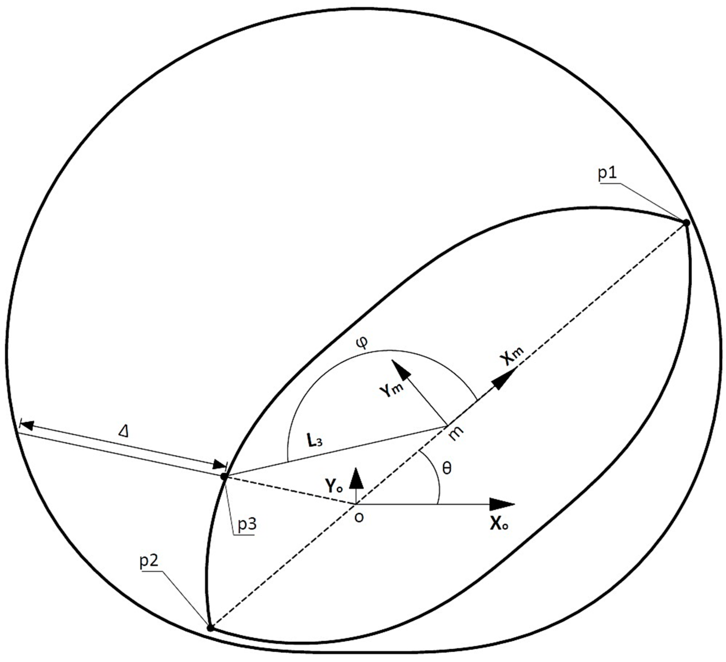
2. Geometric Characteristics of the Limaçon Compressor

One feature distinguishing the limaçon compressor from other types of rotary compressors is that the profiles of the housing and rotor are developed from a mathematical curve named the limaçon of Pascal. In fact, the use of the limaçon technology in fluid machinery can be traced back to the 1800s, but none of those early designs received enough attention from either industrial or academic communities owing to the limitation of manufacturing methods and the lack of mathematical understanding. Over the last two decades, the work of Sultan [15,16,17,18] offered good insights into the limaçon technology, and some studies on the application of the limaçon technology in the gas expander have been reported recently [19,20,21]. However, the investigation of this technology in the compressor is still rarely reported in the available literature. This section is intended to present the geometric characteristics of the limaçon compressor.
Analogous to other types of rotary compressors, the limaçon compressor has advantages such as being compact in size and light in weight. Additionally, the limaçon compressor possesses better sealing performance as the rotor apices are in constant contact with the housing during the operation, and the two-lobe design of the rotor also implies the double-acting nature of the machine. Most distinctively, a larger capacity can be realized by adjusting the limaçon aspect ratio without changing the machine size, thereby allowing for a higher power-to-weight ratio.
Figure 1 below shows a typical limaçon compressor and its working process. As shown in the Figure 1a, the rotor chord, p 1 p 2 , performs sliding and rotational motion about the limaçon pole, o , during its operation. As the rotor moves, the midpoint of the chord, m , is kinematically connected to the circumference of the housing base circle whose radius is r ; the profile of the limaçon housing can be obtained by tracing the path of the chord apex, p 1 or p 2 . To readily describe the parametric coordinates of the chord apices, two Cartesian frames, X o Y o and X m Y m , are respectively introduced at o and m . The housing profile in the X o Y o coordinate can be expressed as:
{ x h = r sin 2 θ + L cos θ                 y h = r r cos 2 θ + L sin θ
where L is half rotor chord length and θ is the angular displacement swept by the chord from the X o - to the X m -axis. It is worthy of mentioning here that the shape of the housing profile is dependent on a geometric factor which is referred to as the limaçon aspect ratio, β = r L . For a limaçon curve that is applicable to fluid machinery, the limaçon aspect ratio needs to be less than 0.25 so that the housing profile can be produced as single-looped and dimple-free.
The lenticular profile of the rotor can be developed by mirroring the lower portion of the limaçon housing (i.e., θ [ π , 2 π ] ) about the chord. However, this could lead to undesirable housing-rotor interference at the lower portion of the housing as the limaçon curves that are respectively used for the housing and rotor profiles share the same base circle. To avoid this interference, it is necessary to shorten the half rotor chord length, L , by a distance L c ; the parametric expression of the rotor with respect to the moving frame, X m Y m , can then be obtained as follows:
{ x r = r r sin θ r + ( L L c ) cos θ r                       y r = r r r r cos 2 θ r + ( L L c ) sin θ r
where r r is the radius of the rotor base circle which is identical to r in this design, and θ r [ π ,   2 π ] is the angle measured from the X m -axis to any point on the rotor profile.
Of important note is that the value of L c needs to be carefully regulated in order to ensure the clearance, Δ , between the housing and the rotor would not fall below a minimum allowable value, Δ m i n , assigned to the design. The expression of Δ has been proposed by Sultan [16] as follows:
Δ = 2 β L 3 sin ( θ φ ) L 3 2 L L 3 2 L 2 + 4 β sin θ ( β sin θ + L 3 L cos φ ) + L
where φ is the angle measured from the X m -axis to the radial line L 3 connecting m to a point p 3 on the rotor profile as shown in Figure 2. L 3 has the expression as follows:
L 3 = 2 r r sin ( φ + π ) + ( L L c )
To obtain an appropriate value for L c which can produce Δ that meets the design requirements, the following conditions must be simultaneously satisfied:
{ Δ θ = 0 Δ φ = 0 Δ Δ m i n 0
The two angles, θ and φ , obtained from Equation (5) are to locate the angular position of the minimum clearance, making sure that Equation (3) using these angles will always yield the lowest value of L c in terms of the proposed Δ m i n .
As shown in Figure 1, the working chamber of the limaçon compressor is separated by the rotor into the upper and the lower portions. Such a configuration implies the fact that the limaçon compressor is a double-acting machine by nature, i.e., the suction process correspondingly occurs in the lower chamber when the discharge process is being conducted in the upper chamber. As such, the limaçon compressor is capable of compressing the working fluid twice per revolution of the crankshaft, and the net volume available for each compression charge can be expressed as a function of θ as follows:
V c = H L 2 [ π ( β 2 r r 2 L 2 + L c L ( 1 L c 2 L ) ) 4 β cos θ + 4 r r L ( 1 L c L ) ]
where H is the axial length of the rotor measured perpendicular to the page.
Equation (6) shows that the variation of chamber volume follows a sinusoidal manner where the maximum and the minimum values are at θ = π and θ = 0 , respectively. Generally, the minimum volume, provided that the rotor-housing clearance condition is satisfied, should be kept as small as practical so that the volumetric performance and machine capacity would not significantly deteriorate. To determine whether the limaçon compressor can present a satisfactory performance, a volumetric ratio, R , is employed. This volumetric ratio, R , is defined as the minimum volume to the maximum volume of the working chamber as follows:
R = π ( β 2 r r 2 L 2 + L c L L c 2 2 L 2 ) 4 ( r r L c L 2 + β r r L ) π ( β 2 r r 2 L 2 + L c L L c 2 2 L 2 ) 4 ( r r L c L 2 β r r L )
In addition, the volume of the working fluid, V i , induced into the chamber by each suction stroke can be used to indicate the machine capacity and which is calculated as:
V i = V c | θ = θ c u t μ V c | θ = 0
where θ c u t ( 0 ,   π ] indicates the end of the suction process. The clearance volume factor, μ , is assigned by the designer to include the effect of residual fluid in the minimum chamber on the suction process. The expression for this factor is shown below:
μ = ρ o ρ i
where ρ i and ρ o are the densities of the fluid flowing in and out of the compressor, respectively. By combining Equations (6) and (8), V i can be expressed in a detailed fashion as follows:
V i = H L 2 ( 1 μ ) [ π ( β 2 r r 2 L 2 + L c L ( 1 L c 2 L ) ) + 4 r r L ( 1 L c L ) ] 4 β H L 2 cos ( θ c u t μ )

3. Mathematical Model

3.1. Mass Flow Rate through the Inlet Port

The mass flow rate through the inlet port can be expressed as:
m ˙ i = ρ i A i u i
where ρ i , u i , and A i are the density, velocity of the fluid, and the instantaneous area of the inlet port at the downstream side, respectively. The computation process of u i and A i can be based on the work of Sultan and Schaller [19].

3.2. Mass Flow Rate through the Discharge Valve

The limaçon compressor is designed with a discharge valve to control the fluid flowing out of the chamber and to prevent backflow from the outlet manifold. The mass flow rate through the discharge valve can be expressed as:
m ˙ v = ρ v A v u v
where ρ v and u v are the density and the velocity of the fluid at the downstream side of the valve, and A v is the effective flow area of the valve obtained from the expression suggested by Tuymer and Machu [22]:
A v = 1 ( 1 0.85 π D v p ( z z m i n ) ) 2 + ( 1 A v p ) 2
where D v p and A v p are the effective diameter and area of the valve plate, respectively. The terms z and z m i n are, respectively, the instantaneous and the minimum displacement of the valve plate; the instantaneous displacement, z , can be obtained from the dynamic model of the discharge valve shown below:
m v p d 2 z d θ 2 = F F r ω 2
In Equation (14), F is the force due to the pressure difference between the two sides of the valve, which is expressed as:
F = C d A v p ( P v c P o t )
where C d is the drag coefficient, P v c and P o t are the pressure in the valve chamber and outlet storage tank, respectively. The resistance force, F r , provided by the spring-damper system (including springs and dampers of the valve, valve seat, and stopper) is calculated in accordance with the valve instantaneous displacement, z , as follows:
F r = { ω ( C v + C s e ) d z d θ + ( k v + k s e ) z k s e z m i n , i f z < z m i n ω C v d z d θ + k v z , i f z m i n < z < z m a x ω ( C v + C s t ) d z d θ + ( k v + k s t ) z k s t z m a x , i f z < z m a x    
where C , k , and z m a x are the damping coefficient, the spring stiffness, and the maximum allowable displacement of the valve, respectively; the subscripts v , s e , and s t represent the valve, the seat, and the stopper, respectively.

3.3. Side and Apex Leakage

For the limaçon compressor, most leakage occurs at the side clearance, the gap between the rotor and the front and back plates of the machine, and apex clearance due to the pressure difference between working chambers. Hence, the total leakage mass flow rate, m ˙ l , is the sum of the side leakage, m ˙ s , and the apex leakage, m ˙ a ,
m ˙ l = m ˙ s + m ˙ a
where the side leakage m ˙ s is calculated using the same approach as m ˙ i (Equation (11)) as shown below:
m ˙ s = ρ s A s u s
where ρ s is the downstream density, A s is the side leakage flow area which is calculated from the half rotor chord length, L , and the side clearance, L s ,
A s = 4 L s L
The apex leakage m ˙ a is formulated by assuming that the leakage through the apex is isentropic flow similar to that of the convergent-divergent nozzle. Apex leakage calculation can be shown as follows:
m ˙ a = { C f A a P a u 2 γ ρ a u ( γ 1 ) P a u [ ( P a d P a u ) 2 γ ( P a d P a u ) γ + 1 γ ] ,     i f       P a d P a u > ( 2 γ + 1 ) γ γ 1 C f A a P a u ρ a u P a u ( 2 γ + 1 ) γ + 1 γ 1                                                             ,     i f       P a d P a u < ( 2 γ + 1 ) γ γ 1
where C f is the flow coefficient, P a u and P a d are the pressure at the upstream and the downstream of the leakage path, respectively, ρ a u is the upstream density at the throat, γ is the specific heat ratio, A a is the leakage flow area at the apex clearance, which is calculated as:
A a = 2 L c H
To reduce the effect of the apex leakage on machine performance, a sealing scheme can be applied to the machine apices. The mathematical model of apex seal and the seal dynamic behavior is detailed in the work of Phung and Sultan [21].

3.4. Thermodynamic Model

By assuming the compressor is working adiabatically, the variation of properties of the working fluid inside each working chamber (i.e., the upper and lower chamber) can be obtained, based on the first law of thermodynamics as well as the conservation of mass, as follows:
d ρ c d θ = 1 V c ω ( m ˙ i m ˙ o m ˙ l 4 ρ c ω β L 2 H sin θ )
d s c d θ = 1 ρ c V c T c ω ( m ˙ i ( h i h c ) m ˙ o ( h o h c ) m ˙ l ( h l h c ) 4 ρ c ω β L 2 H sin θ )
In Equations (22) and (23), ρ c , s c and T c denote density, entropy, and temperature inside the working chamber, respectively, h represents the enthalpy, and the subscripts i , o , and l indicate the inlet port, outlet tank, and leakage, respectively. A more detailed modelling process of the thermodynamic model of the limaçon machine can be found in the work of Sultan [20]. To simulate the behavior of the compressor in one cycle, the above set of differential equations is solved iteratively where the values of various variables are compared at the start and the end of each cycle to signify the cyclical nature of the compressor operation. The comparison is performed with the help of the error function, σ , shown below:
σ = σ 1 + σ 2 + σ 3 + σ 4
where σ 1 , σ 2 , σ 3 and σ 4 are obtained as follows:
σ 1 = ( 2 ( P c A ( θ l i + π ) P c B ( θ ) ) P c A ( θ l i + π ) + P c B ( θ ) ) 2
σ 2 = ( 2 ( P c B ( θ l i + π ) P c A ( θ ) ) P c B ( θ l i + π ) + P c A ( θ ) ) 2
σ 3 = ( 2 ( ρ c A ( θ l i + π ) ρ c B ( θ ) ) ρ c A ( θ l i + π ) + ρ c B ( θ ) ) 2
σ 4 = ( 2 ( ρ c B ( θ l i + π ) ρ c A ( θ ) ) ρ c B ( θ l i + π ) + ρ c A ( θ ) ) 2
where superscripts A and B represent the upper chamber and the lower chamber, respectively. If the error function is not small enough, the parameters at the end of the cycle are employed as initial conditions in the following iteration.

3.5. Simulation of the Limaçon Compressor

In this section, a simulation of the limaçon compressor is presented based on the mathematical models above. Air is selected as the working fluid and the assumption of geometric parameters used in the simulation is listed in Table 1. The ambient temperature is assumed at 20   ° C and the inlet and outlet pressure are set as P i = 100   kPa and P o = 300   kPa , respectively. The operating speed of the crankshaft is assumed at 1400   rpm in the simulation. The simulation is conducted for one working cycle and Figure 3 depicts the variation of some properties, including the pressure and temperature of fluid, the volume of the working chamber, and the torque.

3.6. Performance Indices

The performance of a rotary compressor is usually described by a series of indices. In the present study, the performance of the limaçon compressor is indicated by two of the most used performance indices, which are the isentropic efficiency, η i s , and the volumetric efficiency, η v o l . The isentropic efficiency is defined in this paper as the ratio of the ideal work to the actual work, which can be written in terms of enthalpies, as shown in Equation (29):
η i s = ( h o h i ) ( h o , a c t u a l h i )
where h o ,   a c t u a l is the actual enthalpy at the discharge manifold.
Another performance index used in the current study is the volumetric efficiency, which is the ratio of the actual suction mass of fluid to the amount of fluid, m i d , ideally drawn into the chamber, as shown in Equation (30):
η v o l = m i m i d
The ideal mass of fluid processed per working cycle is given as:
m i d = 2 ρ i V s
where V s is the swept volume and it is calculated as:
V s = V c ( π ) V c ( 0 )
For each working cycle, the total mass of the fluid flowing into the chamber can be calculated as per Equation (33) below:
m i = 2 δ θ ( n = 1 N ( m ˙ i A + m ˙ i B ) n ( m ˙ i A ) n ( m ˙ i A ) 1 2 ( m ˙ i B ) n ( m ˙ i B ) 1 2 )
where δ θ is the size of the angular interval, n is the successive point, and N is the total number of intervals. It is worth mentioning here that the multiplication of a factor of 2 appears in Equations (31) and (33) due to the double-acting nature of the machine.

4. Optimization Process

4.1. Bayesian Optimization Method

Bayesian optimization is a class of surrogate-based global optimization targeting to find the minima (or maxima) of an output y over an input x in a domain 𝕕 , and it can be concisely expressed as follows:
x = argmin x     𝕕 y
where the mathematical expression underlying the relationship between x and y cannot readily be explicitly defined. In practice, Bayesian optimization starts with building a prior distribution based on observations to express assumptions about the black box objective function. It is necessary to point out that the actual value of the function generally differs from the observed one as errors occurring in aspects, such as recording or measuring, are not avoidable. Therefore, the optimization procedure will be more realistic if the observation used to develop the prior distribution is added up with a noise factor, ε , such that those errors can be considered into the process, and the actual function value y is then calculated as
y = f + ε
where f is the observed function value.
Suppose that there are n sets of observation have been made, Bayesian optimization employs statistical methods, particularly Gaussian Process (GP), to sample the observations, which is associated with the input x as follows [23],
f = ( K x + σ 2 I ) w
where σ is the standard deviation, I is the identity matrix, w is a vector of weights, and K x is the covariance matrix that has the form
K x = [ k ( x 1 ,   x 1 ) k ( x 2 ,   x 1 ) k ( x n ,   x 1 ) k ( x 1 ,   x 2 ) k ( x 1 ,   x n ) k ( x n ,   x n ) ]
In Equation (37), each element in the matrix is a covariance function that describes the relationship between points x i and x j ( i , j = 1 , 2 , , n ). For the optimization of the limaçon compressor, the M a t é r n   5 / 2 covariance function is used, which has the form
k ( x i ,   x j ) = c 1 ( 1 + 5 l 2 ( x i ,   x j ) + 5 3 l 2 ( x i ,   x j ) ) exp ( 5 l 2 ( x i ,   x j ) )
where l 2 ( x i ,   x j ) = n ( x i x j ) 2 c 2 2 is the radial basis function, and c 1 and c 2 are the hyperparameters.
Given that one seeks to predict the function value at a new point x * , one can set up the relation between x * and observed points as follows,
K x * = [ k ( x * ,   x 1 ) k ( x * ,   x 2 ) k ( x * ,   x n ) ]
The predicted function value at the point x * can then be computed as
f * = [ K x * ] T ( K x + σ 2 I ) 1 f
In Bayesian optimization, Equation (40) is referred to as the surrogate model of the objective function, and the variance σ * 2 that describes the uncertainty on the prediction can be calculated as
σ * 2 = k ( x * , x * ) [ K x * ] T ( K x + σ 2 I ) 1 K x *
Based on the above equations, the objective function can be evaluated at any input point, and the obtained function value can be verified by using the selected input in the real process. From the optimization point of view, however, it would be time-consuming and wasteful if the evaluation is conducted on any point that is arbitrarily selected in the searching domain. As such, Bayesian optimization employs the acquisition function to guide the search of the next query point. The mechanism of the acquisition function for selecting the next query point is based on the prediction ( f * ) and the uncertainty ( σ * 2 ) of the candidate point. In fact, the acquisition function can be regarded as the examiner of a scoring process. With low prediction (for minimization problems) and high uncertainty, the candidate point obtains a high score from the acquisition function, and the candidate point with the highest score will be selected as the next query point.
Currently, there are many available acquisition functions, e.g., Probability of Improvement (PI) and the Expected Improvement (EI). For the optimization of the limaçon compressor, the scaled expected-improvement acquisition function (ScaledEI) is used [24], which has the following form
S c a l e d E I ( x * ) = E I ( x * ) V I ( x * )
In Equation (42), E I is the normal expected-improvement acquisition function that takes the form:
E I ( x * ) = { ( f m i n f * ) Φ ( Z ) + ϕ ( Z ) σ * ,       i f   σ * > 0 0 ,       i f   σ * = 0
where f m i n is the minimum function value that is observed, Φ and ϕ denote the probability density function and cumulative density function, respectively, and Z is expressed as:
Z = f m i n f * σ *
The term V I in Equation (42) is the variance of the improvement quantifier, which has the form:
V I ( x * ) = σ * 2 ( Z 2 + 1 ) Φ ( Z ) + ( Z ) ϕ ( Z ) E I ( x * ) 2
A comprehensive explanation of ScaledEI can be sought in the work by Noè and Husmeier [24].
Subsequently, the selected query point and its corresponding function value of the real process will be used to update the GP and the process will be repeated till the terminating criteria are satisfied. This also reveals another feature of the Bayesian optimization technique, that is the knowledge of the surrogate function is kept updating along the optimization process, thereby refining the surrogate model.

4.2. Two-Stage Optimization

The optimization of the limaçon compressor in this paper employs the Bayesian optimization presented in the above section. Due to the fact that that the thermodynamic model is complex and computationally intensive, the optimization procedure is implemented by a two-stage process to reduce the computation cost of the overall optimization process. The first stage is to optimize the geometric parameters, including the half chord length, L , the limaçon aspect ratio, β , and the rotor clearance, L c , to meet the specified design requirements. The obtained outcome is evaluated in terms of an evaluation function shown below:
E o 1 = w 1 F 1 + w 2 F 2 + w 3 F 3  
where w 1 , w 2 , and w 3 are weighting factors assigned by the designer to highlight the significance of the corresponding term in the evaluation; F 1 , F 2 , and F 3 are evaluation functions of design requirements associated with Δ , R and V i , which are respectively expressed as follows:
{ F 1 = R R r e q F 2 = V i V r e q F 3 = Δ Δ r e q
where the subscript r e q denotes the design requirement. One should note that Δ used in F 3 is the lowest value of the rotor-housing clearance in terms of the proposed outcome. Therefore, conditions in Equation (5) must be satisfied on top of Equation (47), and the input vector of design variables for the first stage, x o 1 , is then given as:
x o 1 = [ L β L c   ] T
In the first stage, 10 sets of x o 1 will be randomly generated and the corresponding E o 1 will be calculated by using the geometric model proposed in Section 2. These pre-collected data will be regarded as observations that are employed by GP to build the surrogate model. Subsequently, 1500 sets of new input points, x o 1 * , will be sampled from the search domain and feed to the acquisition function to determine the next query point. The determined query point will be then used to calculate the corresponding E o 1 * , which will be saved and used to update the GP till the terminating criteria are reached. When the terminating criteria are satisfied, the machine size will be determined based on the x o 1 * that achieves the lowest value of the recorded E o 1 * , and the second stage optimization will be implemented on top of these geometric parameters to improve the machine performance by modifying the setting of the inlet and outlet ports by utilizing the thermodynamic model presented in Section 3.4. The design variables of this stage, x o 2 , is given as follows:
x o 2 = [ θ l i θ l o Δ θ i         Δ θ o L p i L p o ] T
where θ l , Δ θ , and L p are the angular location of the port leading edge measured from the X o -axis, the port angular width, and the port length, respectively; the subscript i and o represent the inlet port and the outlet port, respectively. The evaluation function of this stage is given by incorporating the performance indices (i.e., isentropic efficiency, η i s , and volumetric efficiency, η v o l ) obtained from the mathematical model:
E o 2 = w 4 ( 1 η i s ) 2 + w 5 ( 1 η v o l ) 2  
where w 4 and w 5 are weighting factors assigned by the designer. The steps of the second stage are similar to that of the first stage, except that 20 sets of x o 2 * and the corresponding E o 2 * will be collected before initiating the optimization process. It should be mentioned here that it is relatively impractical to extract the exact combination of design variables that can produce the global optimum of E o 1 * and E o 2 * due to the high complexity of the relationship between design variables and design objectives. Instead, a more feasible way is that the optimum outcome is reflected by a set of results obtained from the optimization procedure. Figure 4 illustrates the process of the two-stage optimization employed in the current study.

5. Numerical Illustration

In this section, a numerical illustration is presented, and assumptions of the optimization process, such as operating conditions and weighting factors, are listed in Table 2. Mathematically, the searching domain of design variables can be simply set according to the corresponding geometric constraints, e.g., L [ 0 , + ] . For a real compressor, however, it is unrealistic for L to be zero or a very large value. Hence, by considering the actual design situation, the searching domain of each design variable is selected, as shown in Table 3.
Figure 5a depicts a histogram that shows the distribution of E o 1 based on results obtained from the first stage. It is clear that the majority of the result is concentrated in the low-value region (i.e., the first cluster in the figure), indicating that the proposed optimization tends to produce promising outcomes. Figure 5b–d present the distribution of each design variable that yields the result of the first cluster of Figure 5a, which provides useful information to guide the setting of design variables in order to obtain an optimum outcome. The combination of design variables that achieve the minimum E o 1 is used to calculate objective parameters, which are compared with the design requirements as shown in Table 4. With the selected design variables, the limaçon compressor is designed with a volumetric displacement of 720   cm 3 per revolution of the crankshaft.
Figure 6 depicts the distribution of E o 2 , which exhibits a similar pattern to that of E o 1 . The distribution of design variables of the second stage is presented in Figure 7. Based on the first cluster of Figure 6, the optimization yields an average isentropic efficiency of 93.81 % , peaking at 97.05 % and an average volumetric efficiency of 83.62 % with the highest of 86.99 % .
Based on the results, the designer will obtain a range for every design parameter from which an acceptable design can be manufactured. However, it should be pointed out that the optimization is conducted by assuming the compressor is working under a constant operating speed and pressure ratio, making the optimum design only valid for the given working condition. In actual applications, the machine is generally required to handle various tasks while maintains acceptable performance; therefore, it is necessary to evaluate the design under different working conditions. In the current work, the result whose design variables achieve the minimum E o 1 and E o 2   is considered as the optimum design. Figure 8 shows the performance of the proposed optimum design with respect to different speeds of the crankshaft. It is found that the optimum design can exhibit relatively stable performance when the speed varies within a small percentage around that used in the optimization. Figure 9 depicts the machine performance under different outlet pressure. It is obvious that the isentropic efficiency is not sensitive to the changes occurring in the outlet pressure, as reflected by the nearly flat curve in Figure 9. For the volumetric efficiency, it decreases as the outlet pressure increases, but the reduction is not significant when the outlet pressure fluctuates around the value used in the optimization, thus suggesting a reasonable level of robustness. Based on Figure 8 and Figure 9, the best performance is found to be 99.09 % for isentropic efficiency and 86.25 % for volumetric efficiency, and they are compared with the reported performance of other types of rotary compressors to highlight the significant potential of the limaçon compressor, as shown in Table 5.

6. Conclusions

In this paper, the Bayesian optimization technique is applied in a two-stage optimization process of the limaçon compressor, where the first stage determines the size of the compressor as per design requirements and the second stage aims to optimize the setting of the port to improve machine performance. The results of the numerical illustration prove the validity of the proposed method for the given design tasks with obtaining satisfactory machine performance. Additionally, a discussion is presented on the effects of operating parameters (pressure ratio and speed) on the performance of the optimized design. It is found that the optimized design exhibits relatively stable isentropic efficiency over the tested range of the speed and the outlet pressure, whereas volumetric efficiency can be maintained within an acceptable range when the operating condition is around that used in the optimization. This provides the designer useful information on the suitable operating conditions for the optimized design in real applications, and more importantly, it highlights the importance of the optimization process before the prototype is produced for a specific application.

Author Contributions

Conceptualization, K.L., T.H.P. and I.A.S.; methodology, K.L., T.H.P. and I.A.S.; software, K.L., T.H.P. and I.A.S.; validation, K.L.; formal analysis, K.L.; investigation, K.L.; resources, T.H.P. and I.A.S.; data curation, K.L.; writing—original draft preparation, K.L.; writing—review and editing, K.L., T.H.P. and I.A.S.; visualization, K.L.; supervision, T.H.P. and I.A.S.; project administration, T.H.P. and I.A.S.; All authors have read and agreed to the published version of the manuscript.

Funding

This research was funded by Findlay Engineering Pty Ltd. under FedUni research project number (G2037).

Institutional Review Board Statement

Not applicable.

Informed Consent Statement

Not applicable.

Data Availability Statement

Not applicable.

Conflicts of Interest

The authors declare no conflict of interest.

References

  1. Ooi, K. Design optimization of a rolling piston compressor for refrigerators. Appl. Therm. Eng. 2005, 25, 813–829. [Google Scholar] [CrossRef]
  2. Liu, Y.; Hung, C.; Chang, Y. Design optimization of scroll compressor applied for frictional losses evaluation. Int. J. Refrig. 2010, 33, 615–624. [Google Scholar] [CrossRef]
  3. Sultan, I.; Kalim, A. Improving reciprocating compressor performance using a hybrid two-level optimisation approach. Eng. Comput. 2011, 28, 616–636. [Google Scholar] [CrossRef]
  4. Phung, T.H.; Sultan, I.A. Geometric Design of the Limaçon-to-Circular Fluid Processing Machine. J. Mech. Des. 2021, 143, 103501. [Google Scholar] [CrossRef]
  5. Cavazzini, G.; Giacomel, F.; Ardizzon, G.; Casari, N.; Fadiga, E.; Suman, A.; Pinelli, M. CFD-based optimization of scroll compressor design and uncertainty quantification of the performance under geometrical variations. Energy 2020, 209, 118382. [Google Scholar] [CrossRef]
  6. Silva, E.; Dutra, T. Piston trajectory optimization of a reciprocating compressor. Int. J. Refrig. 2021, 121, 159–167. [Google Scholar] [CrossRef]
  7. Aw, K.T.; Ooi, K.T. A Review on Sliding Vane and Rolling Piston Compressors. Machines 2021, 9, 125. [Google Scholar] [CrossRef]
  8. Pelikan, M.; Goldberg, D.E.; Cantú-Paz, E. BOA: The Bayesian optimization algorithm. In Proceedings of the Genetic and Evolutionary Computation Conference, Orlando, FL, USA, 13–17 July 1999; Volume 1, pp. 525–532. [Google Scholar]
  9. Snoek, J.; Larochelle, H.; Adams, R.P. Practical Bayesian optimization of machine learning algorithms. In Proceedings of the Advances in Neural Information Processing Systems, Lake Tahoe, NA, USA, 3–6 December 2012; pp. 2951–2959. [Google Scholar]
  10. Frazier, P.I.; Wang, J. Bayesian optimization for materials design. In Information Science for Materials Discovery and Design; Lookman, T., Alexander, F.J., Rajan, K., Eds.; Springer: Berlin/Heidelberg, Germany, 2016; pp. 45–75. [Google Scholar]
  11. Torun, H.; Swaminathan, M.; Kavungal Davis, A.; Bellaredj, M. A Global Bayesian Optimization Algorithm and Its Application to Integrated System Design. IEEE Trans. Very Large Scale Integr. (VLSI) Syst. 2018, 26, 792–802. [Google Scholar] [CrossRef]
  12. Griffiths, R.R.; Hernández-Lobato, J.M. Constrained Bayesian optimization for automatic chemical design. arXiv 2017, arXiv:1709.05501. [Google Scholar]
  13. Letham, B.; Karrer, B.; Ottoni, G.; Bakshy, E. Constrained Bayesian Optimization with Noisy Experiments. Bayesian Anal. 2019, 14, 495–519. [Google Scholar] [CrossRef]
  14. Hickish, B.; Fletcher, D.; Harrison, R. Investigating Bayesian Optimization for rail network optimization. Int. J. Rail Transp. 2019, 8, 307–323. [Google Scholar] [CrossRef] [Green Version]
  15. Sultan, I.A. The Limaçon of Pascal: Mechanical Generation and Utilization for Fluid Processing. Proc. Inst. Mech. Eng. Part C J. Mech. Eng. Sci. 2005, 219, 813–822. [Google Scholar] [CrossRef] [Green Version]
  16. Sultan, I.A. Profiling Rotors for Limaçon-to-Limaçon Compression-Expansion Machines. J. Mech. Des. 2006, 128, 787–793. [Google Scholar] [CrossRef]
  17. Sultan, I.A. A Surrogate Model for Interference Prevention in the Limaçon-to-Limaçon Machines. Eng. Comput. 2007, 24, 437–449. [Google Scholar] [CrossRef]
  18. Sultan, I.A. Inverse geometric design for a class of rotary positive displacement machines. Inverse Probl. Sci. Eng. 2008, 16, 127–139. [Google Scholar] [CrossRef]
  19. Sultan, I.A.; Schaller, C. Optimum Positioning of Ports in the Limaçon Gas Expanders. J. Eng. Gas Turbines Power 2011, 133. [Google Scholar] [CrossRef]
  20. Sultan, I.A. Optimum design of limaçon gas expanders based on thermodynamic performance. Appl. Therm. Eng. 2012, 39, 188–197. [Google Scholar] [CrossRef]
  21. Phung, T.; Sultan, I.; Appuhamillage, G. On the apex seal analysis of limaçon positive displacement machines. Mech. Mach. Theory 2018, 127, 126–145. [Google Scholar] [CrossRef]
  22. Tuymer, W.J.; Machu, E.H. Compressor valves. In Compressor Handbook; Hanlon, P.C., Ed.; McGraw-Hill: New York, NY, USA, 2001. [Google Scholar]
  23. Rasmussen, C.E.; Williams, C.K.I. Gaussian Processes for Machine Learning; MIT Press: Cambridge, MA, USA, 2006. [Google Scholar]
  24. Noè, U.; Husmeier, D. On a new improvement-based acquisition function for Bayesian optimization. arXiv 2018, arXiv:1808.06918. [Google Scholar]
  25. Cuevas, C.; Lebrun, J.; Lemort, V.; Winandy, E. Characterization of a scroll compressor under extended operating conditions. Appl. Therm. Eng. 2010, 30, 605–615. [Google Scholar] [CrossRef]
  26. Pan, X.; Tian, C.; Wu, S.; Xing, Z.; Pan, S. Experimental study of the swing compressor with no valves. Appl. Therm. Eng. 2019, 163, 114274. [Google Scholar] [CrossRef]
  27. Shakya, P.; Ooi, K. Introduction to Coupled Vane compressor: Mathematical modelling with validation. Int. J. Refrig. 2020, 117, 23–32. [Google Scholar] [CrossRef]
  28. Wang, J.; Liu, Y.; Chen, Z.; Tan, Q. Geometric model and pressurization analysis on a novel sliding vane compressor with an asymmetrical cylinder profile. Int. J. Refrig. 2021, 129, 175–183. [Google Scholar] [CrossRef]
Figure 1. (a) The limaçon compressor; (b) illustration of the working process (suction is blue and delivery is red).
Machines 09 00219 g001aMachines 09 00219 g001b
Figure 2. The rotor-housing clearance.
Machines 09 00219 g002
Figure 3. Variation of fluid properties; (a) pressure; (b) temperature; (c) volume; and (d) torque.
Machines 09 00219 g003
Figure 4. Illustration of the two-stage optimization process.
Machines 09 00219 g004
Figure 5. Result of the first stage: (a) distribution of E o 1 ; and distribution of first stage design variables: (b) half chord length; (c) aspect ratio; (d) rotor clearance.
Machines 09 00219 g005
Figure 6. Distribution of E o 2 .
Machines 09 00219 g006
Figure 7. Distribution of second stage design variables: (a) leading edge of inlet port; (b) leading edge of outlet port; (c) inlet port angular width; (d) outlet port angular width; (e) inlet port length; (f) outlet port length.
Machines 09 00219 g007aMachines 09 00219 g007b
Figure 8. Performance of the optimized compressor under different speeds (at P o = 300   kPa ).
Machines 09 00219 g008
Figure 9. Performance of the optimized compressor under different outlet pressure (at 1400   rpm ).
Machines 09 00219 g009
Table 1. Geometric parameters used in the simulation.
Geometric ParametersValues
Half-length of the rotor-chord, L 0.0517   m
Axial length of the rotor, H 0.0672   m
Rotor clearance, L c 1   mm
Side clearance, L s 0.01   mm
Aspect ratio, β 0.1
Leading edge of inlet port, θ l i 7.5 °
Leading edge of outlet port, θ l o 175 °
Angular width of inlet port, Δ θ i 11 °
Angular width of outlet port, Δ θ o 10 °
Length of inlet port, L p i 0.0336   m
Length of outlet port, L p o 0.0222   m
Table 2. Assumptions of the optimization process.
ParametersValue
Speed of the crankshaft 1400   rpm
Temperature at inlet port, T i 20   ° C
Pressure at inlet port, P i 100   kPa
Pressure at outlet port, P o 300   kPa
Clearance volume factor, μ 5
Cut-off angle of the suction process, θ c u t π
Weighting factors w 1 1
w 2 1000
w 3 100
w 4 1
w 5 1
Table 3. The searching domain of each design variable.
Design VariableLower LimitUpper Limit
Half chord length, L 0.04   m 0.15   m
Aspect ratio, β 0.04   0.22
Rotor clearance, L c 0.5   mm 1.5   mm
Leading edge of inlet port, θ l i 7.5 ° 3 °  
Leading edge of outlet port, θ l o 175 ° 200 °
Angular width of inlet port, Δ θ i 4 ° 16 °
gular width of outlet port, Δ θ o 4 ° 16 °
Length of inlet port, L p i 0.02   m 0.09   m
Length of outlet port, L p o 0.02   m 0.09   m
Table 4. Comparison of obtained result and required result.
Objective ParametersRequired ValueObtained Value
Volume ratio, R 0.02 0.0193
Induced volume per suction process, V i 3 × 10 4   m 3 3.316 × 10 4   m 3
Rotor-housing clearance, Δ 5 × 10 4   m 5.9 × 10 4   m
Table 5. Performance comparison of other types of rotary compressors.
TypeVolumetric Displacement per RevolutionWorking FluidReported Maximum Performance
Limaçon 720   cm 3 Air 86.25 %   ( V o l u m e t r i c ) ,  
99.09 %   ( i s e n t r o p i c )
Hermetic scroll [25]-R134A 72 %   ( I s e n t r o p i c )
Swing-vane [26] 10.49   cm 3 R410A 91 %   ( V o l u m e t r i c ) ,  
79 %   ( I s e n t r o p i c )
Coupled-vane [27] 44   cm 3 Air 79 %   ( V o l u m e t r i c )
Asymmetrical sliding vane [28] 1.79   cm 3 Air 73.27 %   ( V o l u m e t r i c )
Publisher’s Note: MDPI stays neutral with regard to jurisdictional claims in published maps and institutional affiliations.

