1. Introduction
The adoption of electrified systems is one of the biggest challenge of the automotive industry and this has led to many research activities dealing with their development and criticalities, [
1,
2,
3]. A way to improve fuel economy and performance of motor vehicles is to adopt hybrid architectures [
4]. Hybrid electric vehicles (HEV) work in several operating modes: fully electric; charge sustaining; stationary condition; braking regeneration [
5]. Considering these scenarios, a power-split transmission and a compound power-split electric continuously variable transmission (eCVT) have been introduced to improve the global efficiency of the system. HEVs are often equipped with multiple power sources so transmissions with multiple inputs are often employed as the power split transmissions (PS-CVT) [
6]. Among them, the input split type shows good efficiency in the overall shifting ranges [
7] and it is the most suitable split system for single mode hybrid powertrains. However, single mode powertrains of input split type, show low efficiency at high vehicle speeds [
7,
8]. In dual mode powertrains, the power split type can be selected engaging or disengaging a clutch included in the transmission layout. The availability of two transmission modes overcome the problems of the single mode powertrain, providing better vehicle performance in terms of fuel economy, acceleration and motor size [
9,
10,
11]. Beside the input power split eCVT, there are more complex solutions with several transmission modes considering, in the system layout, at least two epicyclical gear trains and one or more locking system [
12,
13,
14]. These solutions can be classified as compound type power split and examples are given by the devices developed by Allison, Timken, Renault, Toyota and by the GM/Daimler/BMW joint project called Global Hybrid Cooperation [
5].
A proper modelling and simulation tool is very important in the early design and analysis stage. This is even more critical for the power-split HEVs due to the numerous available configurations/components and various control strategies [
15,
16,
17]. Our research group has recently studied the power flows and efficiency of the Power Split CVT [
8,
18,
19]. The powers flowing in the different paths of the PS-CVT have been evaluated in the two possible directions [
8].
The results of the above-mentioned analysis were that the efficiency depends on the power flow types and the overall losses are minimized through a type I power flow, in a series-PS-CVT and type II power flow in a parallel-PS-CVT. The selection of the PS-CVT type, series or parallel, strongly depends on the transmission ratio limits in the concept phase. The type II flow leads to higher efficiencies with low transmission ratio values whilst type I flows ensures higher efficiency and input powers selecting high global transmission ratio values.
In this work, an analytical method to evaluate the power flows and the efficiency of “four-port-mechanical-power split device” is proposed. The purpose of this work is to provide a useful tool to obtain an optimal design of the control system through a general and complete model of the efficiency of transmission. The selected compound architecture consists of an eCVT connecting two planetary gears (PG1, PG2). The internal power circulations are determined through a dynamic analysis of the four-port Compound eCVT. Finally, an analytical expression of the efficiency of the compound transmission is shown, considering that the only dissipative device of the compound is the eCVT variator.
2. Kinematics Analysis of Compound Power-Split CVU
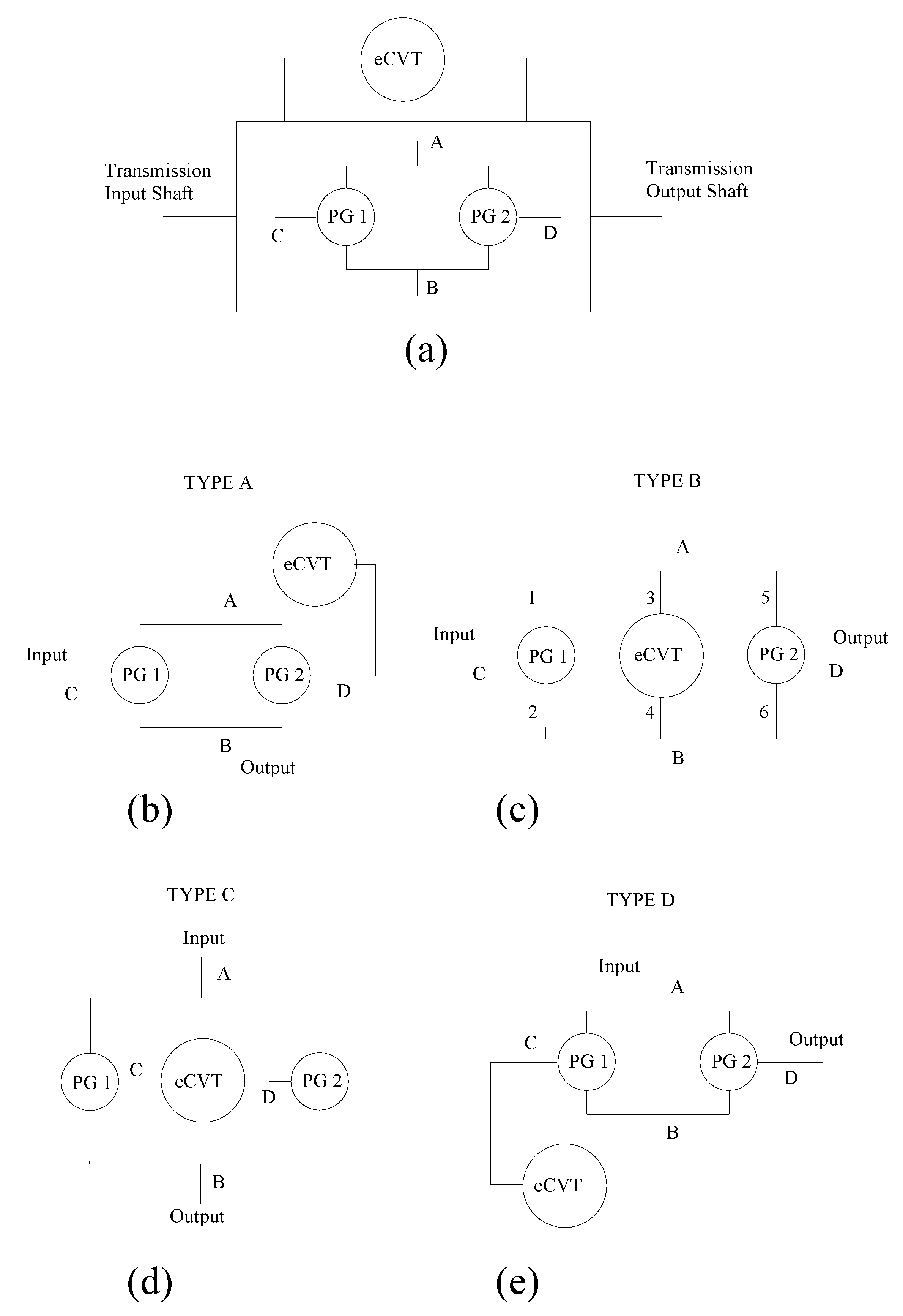
A compound power-split CVU consists of an eCVT and one power split device. The eCVT system is obtained connecting two electric motors, named M1 and M2 as schematically shown in
Figure 1a ([
18]), whilst the two planetary gear sets, named PG 1 and PG 2 in
Figure 1, act as mechanical power split device. In this work, the combination of these system has been named ‘Four-port mechanical power-split device’ and the available four set-ups are shown in
Figure 1b–e. In [
18,
19], the type A and D arrangements (
Figure 1b,e) have been analysed and discussed due to their possible application on heavy vehicles such as large buses, trucks. The compound power-split transmission discussed in this work is the “Type B” layout,
Figure 1c, in which the input and output shafts are connected to the two planetary gear trains.
In the schematic layout, the shafts are numbered from 1 to 6. The definition of the transmission ratios for the PGs and the eCVT is directly obtained:
with:
where
denotes the angular speed of the
ith path. The global speed ratio, named
, is derived rearranging and combining the expressions defined in (1):
From Equation (4) it follows that:
The partial derivative of the global speed ratio with respect to the eCVT speed ratio is always a monotonic function since the sign of Equation (5) changes according to the sign of the numerator, function of the planetary gears characteristic. Equations (4) and (5) are analytical expressions that can be directly used in the early design stage to determine the characteristic values of the planetary gears. eCVTs have a speed ratio ranging from a minimum and a maximum value, named and respectively and these limits are the design inputs, together with the global speed ratio limits, to obtain and .
The overall speed ratio,
, is designed as a monotonic function of the
. If a direct proportion between
and
is selected, the condition in (6) must be verified, starting from the result obtained expression in Equation (5):
If specific minimum and maximum values (
) are required as limits of the global speed ratio, it would be possible to unequivocally compute the transmission ratio of the planetary gear trains using Equation (4), with a given eCVT (
and
known). Imposing a monotonic increase in the expression
, the values
and
are obtained:
The expressions in (7) and (8) are a system of two equations in the two unknown quantities
and
. Solving with respect to
and
:
The same approach can be followed if a monotonic decrease relation is imposed between the global and eCVT speed ratios. In this case, the functions to obtain the planetary gear trains ratios, and , are and , here omitted for brevity. The expressions of and are included in Equations (11) and (12)
3. Power Flow in Compound Power-Split CVU
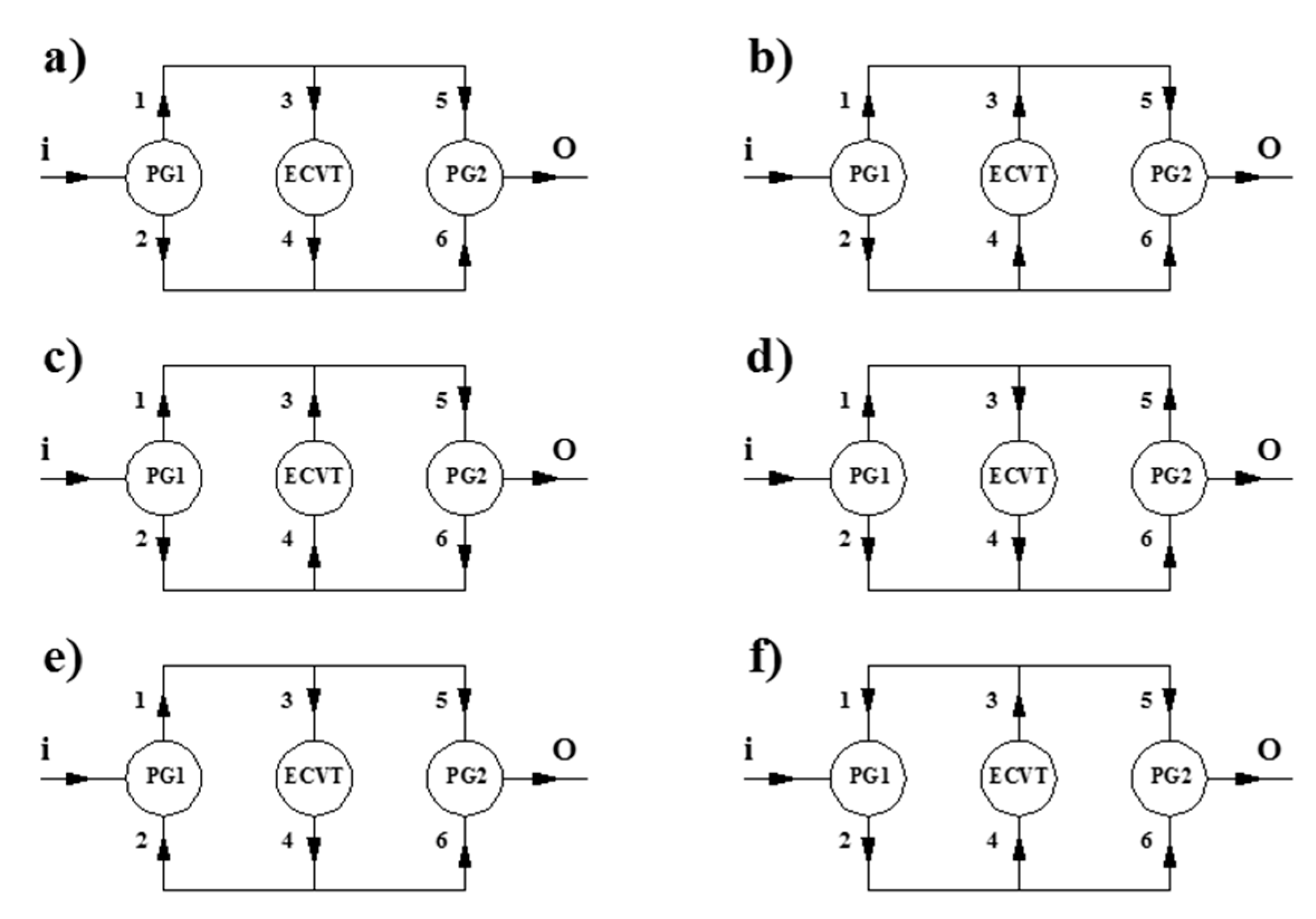
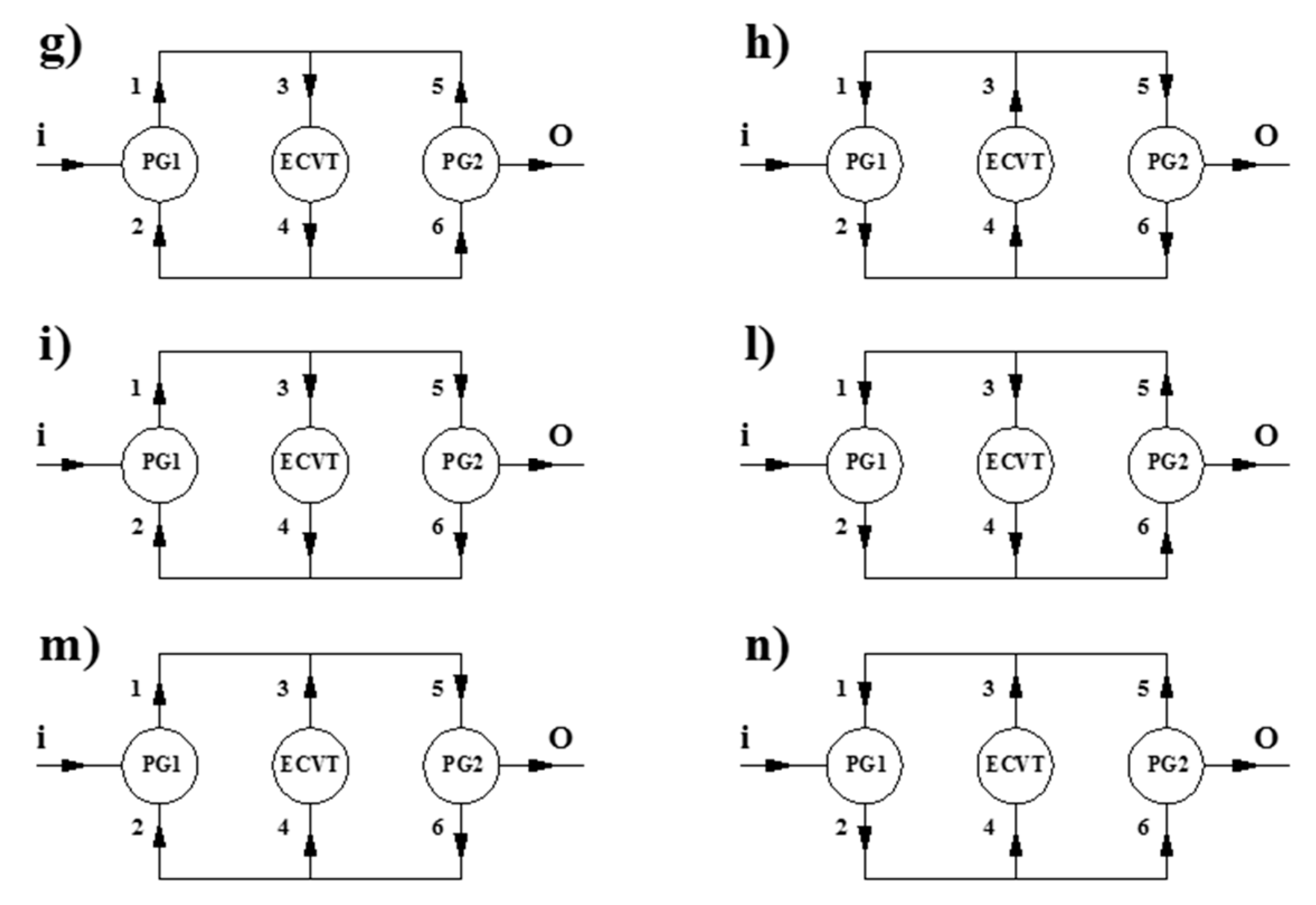
The presence of two planetary gear sets establishes several power flows within the compound system. The possible power flows are schematically described in
Figure 2. Each power flow occurs when specific conditions are verified.
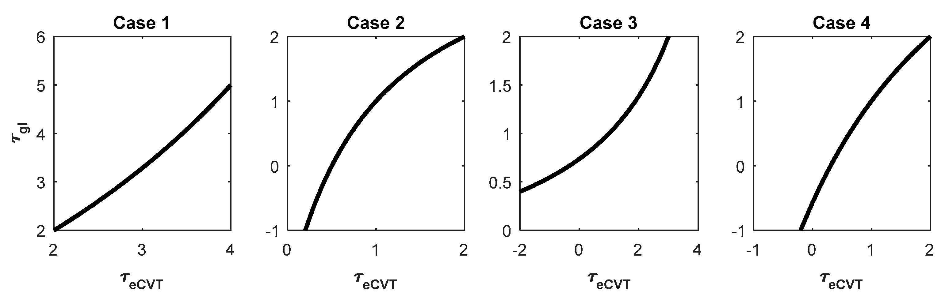
This section deals with the necessary conditions to understand at priori which power flows will occur in the power-split device. These conditions are divided in four cases, depending on the signs of the speed ratios,
and
.
Figure 3 describes, as an example, four cases, functions of the imposed speed ratios limits.
3.1. Case n. 1: e > 0
If
and
are always positive, that is, their operational limits are within positive values:
From Equation (1) the following is obtained:
From Equations (13) and (14) it can be seen that if:
The
and
would tend to infinity when
. Therefore, the values reported in Equation (15) cannot be considered. So,
must be:
If we suppose the planetary gear without losses, the torques ratios of the planetary gear are (
Figure 1):
With the Equations (14) and (17), we obtain the following expressions of the relationships between the powers:
Therefore, if the conditions in Equation (13) are verified, for each of the possible power ratio signs,
Table 1 shows the ranges of the values of
and
. For example,
is positive when
, whilst is negative when
.
Using the results reported in
Table 1, it is possible to uniquely determine the power ratio signs (e.g., the power flows within the transmission as in
Figure 2) knowing the values of
and
.
For example, Type (a) and (b) power flows have an identical condition of
and
(first two rows in
Table 1). However, they are distinguished by the direction of the power in the eCVT (
Figure 1). In particular, type (a) power flow occurs when
. From Equation (17), it is possible to obtain the following equation:
From Equations (4) and (20) it follows:
From Equation (21) and considering
(first row of
Table 2), the type (a) power flow occurs when
, having
. Otherwise, a type (b) power flow occurs when
. The same consideration is repeated for the flows [i − m] and for flows [l − n], since they are distinguished by the direction of the power in the eCVT.
Also for these cases, the last column of
Table 2 shows the additional conditions to distinguish them. In conclusion, known
and
or calculated through Equations (9) and (10) (or Equations (11) and (12), using
Table 2 it is possible to uniquely identify the power flow that is established in the Compound. For example, if
and
the power flow is type (f).
3.2. Case n. 2: ; and
In this case we assume that
is always positive, whilst the
can even reach negative values, meaning that the output shaft speed can reverse its rotating direction. The global speed ratio,
, is equal to zero when
(Equation (4)). Therefore,
could pass from positive to negative values if and only if:
Given that
, it follows:
When the output shaft speed,
, changes its rotating direction (i.e.,
), the sign of the output torque,
, changes accordingly. This implies that the shaft torques in the branches 5 and 6 (
Figure 2), named
respectively, change their sign. Conversely, the sign of the torques
related to the shafts directly connected to the input shaft through the PG 1, remains unchanged since
(input torque) is unchanged. Through Equations (18) and (19),
Table 3 shows the conditions that determine the sign of the power ratios in the two planetary gear sets. The last 2 rows of
Table 3 show the sign of
and
, which changes in the transit from the condition of neutral gear (
), that is, when
.
Using the results of the
Table 3,
Table 4 shows the necessary conditions for the power flows occurrence. The table shows that some power flows are never established if the global speed ratio can assume negative values. From the condition of Equation (23), the power flows named (a), (b), (e) and (f) are automatically excluded since they occur for a negative value of
. Type (i) and (m) power flows have an identical condition of
and
. Considering Equation (23) in addition to the conditions of
e
,
is obtained. This condition is only possible for the type (m) power flow (
Figure 1), that is, the type (i) power flow can never occur. Similarly, Type (l) and (n) power flows have an identical condition of
and
. Then, repeating what has been said before, only type (l) power flow (
Figure 1) is possible, that is, the type (n) power flow can never occur. This is highlighted in the table with grey rows.
In conclusion, taking into account the results shown in
Table 4,
Table 5 summarizes the power flow as a function of
and
. The type of power flow changes when
.
3.3. Case n. 3: ; and
In this case
can be equal to zero meaning that the speed of shaft “B”,
, is null (Equation (1)). When
= 0, the powers in the branches 4, 2 and 6, (
P4 =
P2 =
P6) are equal to 0. Consequentially, from the powers equilibrium
Pi =
P1 =
P5 =
PO and
. For other values of
, the direction of
P1 and
P5 cannot change, because the sign of the torques and angular velocities cannot change. Then, given that
P1 < 0 and
P5 > 0, the possible power flows (
Figure 1) are: Type (a), (b), (c), (e), (i) and (m). Furthermore, it must be:
because, from Equation (4), if Equation (24) is not verified, there would be a
, whilst if the Equation (25) was not verified, it would
. Considering the Equations (18) and (19),
Table 6 shows the conditions on the signs of the powers for case 3.
Using the summary of the conditions presented in
Table 6, the necessary conditions to determine which power flow will occur are described in
Table 7. Also in this case, there are cases in which the data of
Table 6 are not sufficient. For example, in line 1 and 2 of
Table 7 and
are negative and this implies that
and
when
(
Table 6). This condition occurs for type (a) and (b) power flow when
. The condition that can be added to establish the power flow relies on the magnitude of the torques in the branches 1 and 5: Type (a) (
) when
whilst Type (b) (
) when
.
When
, the sign of the powers
and
is reverted (
Figure 1) and it changes from the type (a) power flow to the two possible alternatives type (i) or (m). Taking into account that
remains valid only the type (m) power flow is automatically obtained. Similar considerations can be repeated for the other rows in the
Table 7.
3.4. Case n. 4: and ; and
Case n.4 is the most general one since
and
can be zero (
= 0 or
= 0). In this case scenario, Equation (24) must be verified otherwise there would be an operating condition for which
. Considering that
must be able to assume a null value, from Equation (4) it is possible to obtain:
Table 8 shows the condition on the signs of the powers in the different branches, obtained by means of Equations (18) and (19) together with Equation (24) and (26).
is always negative for the same reasons of the case n.3. The other powers have a sign which depends on the sign of
,
and
.
When
,
Table 9 shows the conditions necessary to obtain the various power flows. The type (f), (h), (l) and (n) power flow cannot occur because it would require
. The type (b) power flow is impossible because it requires (
Figure 1)
, that is,
(Equation (21)). Similar considerations are valid for the type (i) power flow. Also in this case the power flows that never occurs are shown with grey rows.
Table 10 shows the conditions for obtaining the various power flows when
. The results are obtained based on the
Table 8 and Equation (21). In this case, the type (a) and (b) power flows require the same condition for
and
. However, the type (b) (
) power flow does not occur for the Equation (21). Similar considerations can be repeated for the type (m).
Finally, using the results of
Table 9,
Table 10 and
Table 11 summarizes the power flow for different values of
and
. For example, the first row is characterized by
and
. In these conditions, when
the power flow is type (a) (
Table 9). When
the power flow becomes type (i) (row n. 7 in
Table 10). Whereas when
the power flow becomes type (g) (row n. 6 in
Table 10). In conclusion, when
or
changes sign, the type of power flow changes.
In conclusion the
Table 2,
Table 5,
Table 7 and
Table 11 show the type of power flow according to the transmission ratios of the planetary gear train and the eCVT.
The analysis of the four cases has demonstrated the usefulness of this approach in the definition of the power flow within a compound split transmission through kinematic considerations. In summary, the power flow within the system is obtained:
Knowing the kinematic relationship between and
Knowing the parameters of the planetary gears, obtained in the design stage
Knowing the maximum and minimum limits of the eCVT and compound speed ratios
4. Efficiency in Compound Power-Split CVU
In the Compound Power Split device, the power loss is mainly due to the eCVT. Consequently, it is interesting to evaluate the value of the eCVT power. It has been demonstrated in References [
12,
13,
14], that the power through the eCVT branch, divided by the input power of the overall CVU, can be easily calculated, independently on the internal arrangement of the CVU, under the assumption of negligible power loss (ideal CVU), by:
In this hypothesis, the power through the eCVT is:
The overall efficiency can be easily derived under this hypothesis. This assumption is generally accepted, because the efficiency of the eCVT,
is very low (e.g., an electric motor–generator) compared with the other components. Considering the node connecting the eCVT with the shafts 1 and 5 in
Figure 1:
By the Equations (29) and (30), we obtain:
If
(type (a), (d), (e), (g), (i), (l) power flows) the eCVT power loss can be calculated as:
Therefore, the output power is:
By the Equations (31) and (33), we obtain:
Therefore, from Equations (32) and (35):
If
(type (b), (c), (f), (h), (m), (n) power flow) the eCVT power loss can be calculated as:
Similarly to the case above, it is obtained:
Then, the Equations (36) and (39) describe the global efficiency as a function of the eCVT transmission ratio.
5. Example: Power Flows and Efficiency in a Compound Power-Split CVU
In this section, we will evaluate the performance of one example of Compound Power Split CVU. We assume that the input design parameters are:
With a target global speed ratio limits as:
With the value reported in Equations (40) and (41), the values of the planetary gear ratios are derived using by Equations (9) and (10):
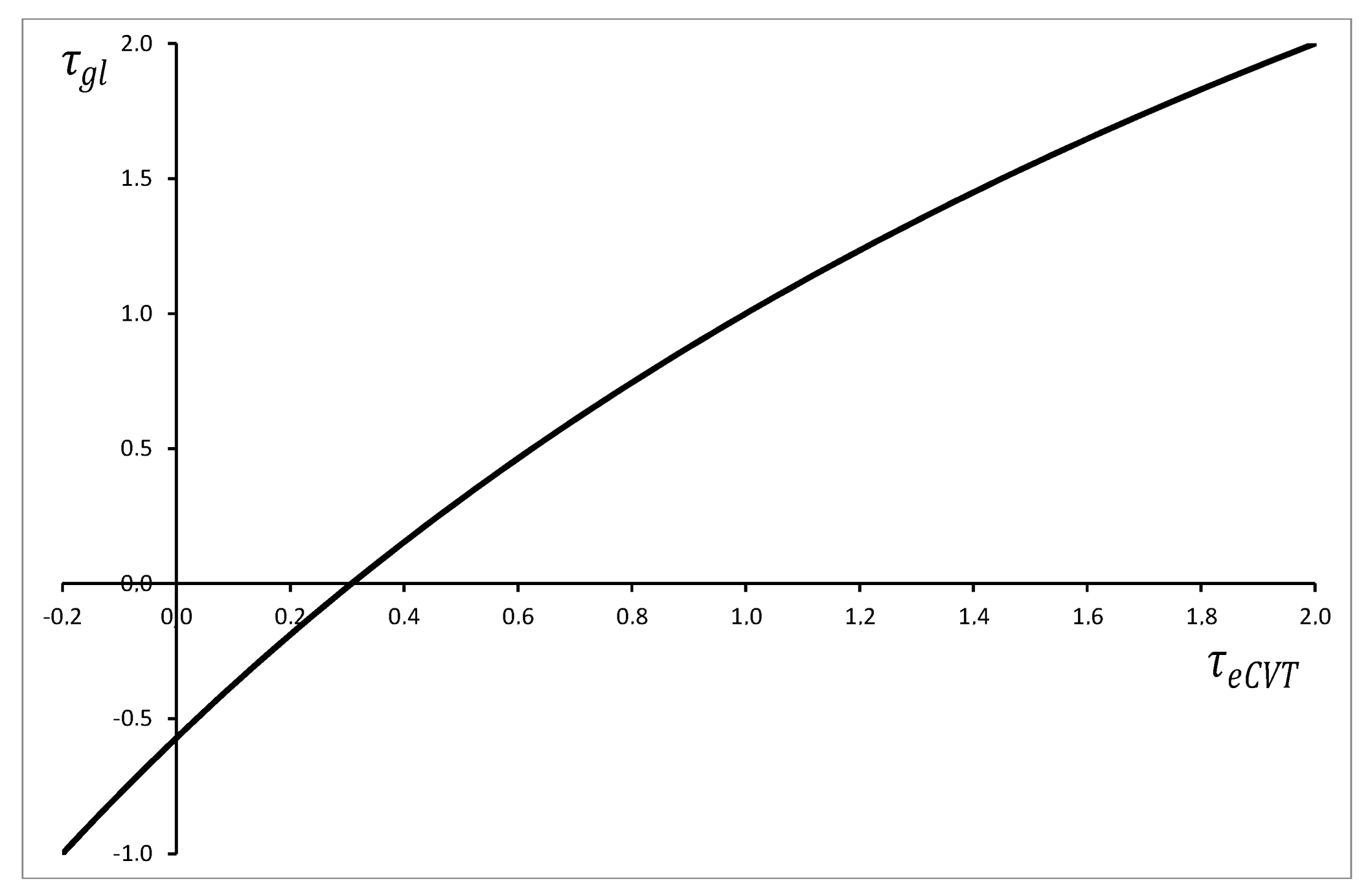
Figure 4 shows
versus
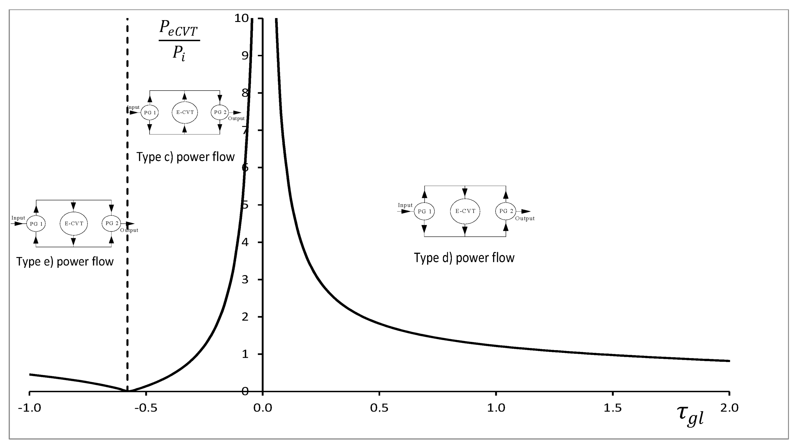
. Of course, the function is increasing, because Equations (9) and (10) have been applied. The power through the eCVT as a function of
(Equation (28)) is shown in
Figure 5, under the assumption of negligible power loss. Three regions can be distinguished in
Figure 5, corresponding to three different ranges of
: the first range
with
; the second range
with
and the third range
with
. Each region corresponds to a different power flow circulation.
In particular, since:
from
Table 11, the power flows are automatically established:
Type (e) power flow when and
Type (c) power flow when and
Type (d) power flow when and
For low values, close to zero, of the global transmission ratio,
, a considerable re-circulating power occurs (
Figure 5). When
and
, the power that circulates through the eCVT is less than the input power.
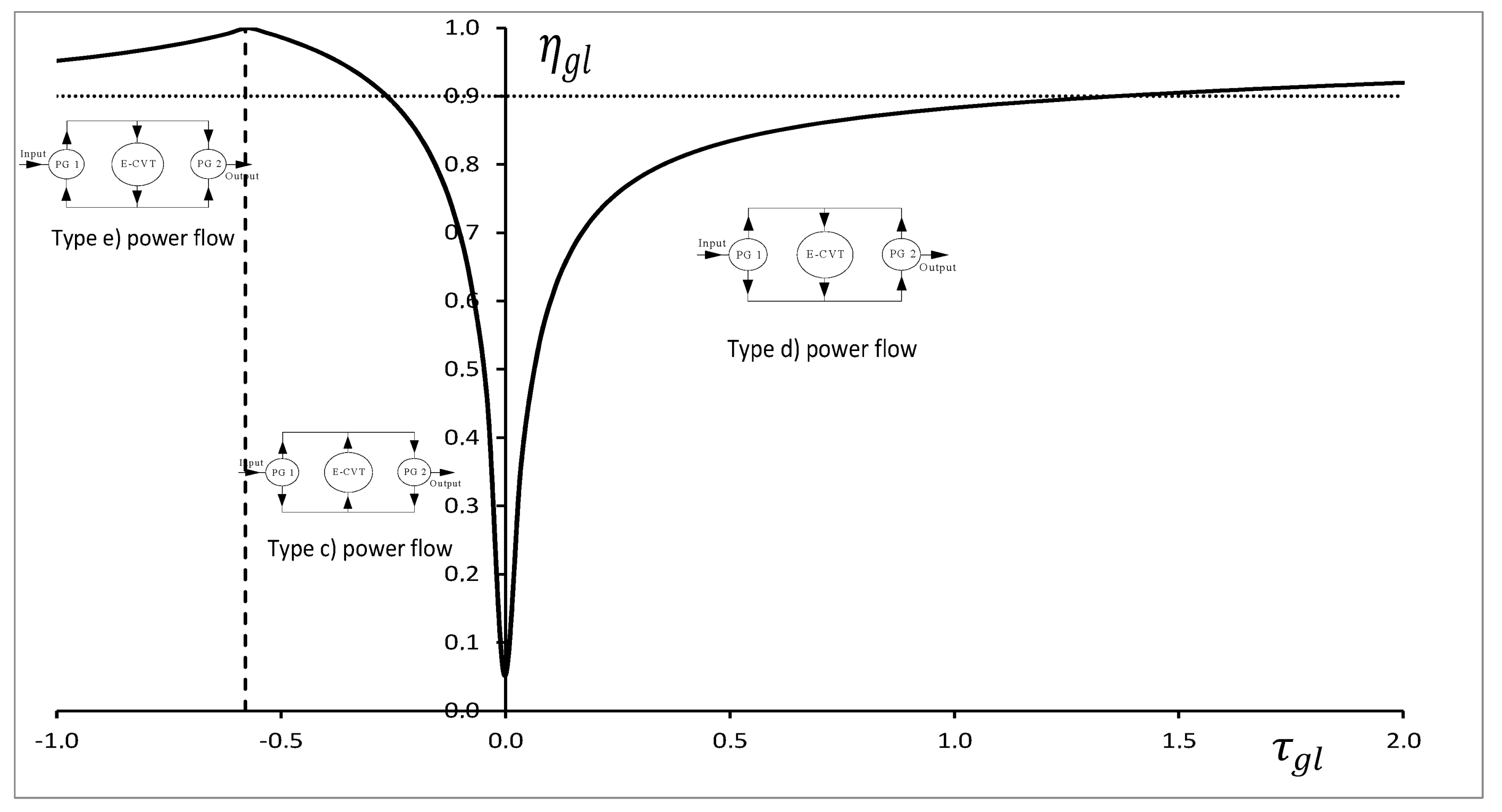
The efficiency of the system, when type (e) and (d) power flow occur, is determined using the expression in Equation (36). Conversely, Equation (39) allows the calculation of the efficiency when the power flow is type (c).
Assuming
,
Figure 6 shows the global efficiency (
) as a function of the overall speed ratio. The overall efficiency decreases near the
equal to zero since the power in the eCVT is asymptotically increasing. When there is no re-circulating power, the global efficiency becomes greater than the one of the eCVT. The example here presented gives an indication on how to derive an optimal energy management of the power-split transmission. Generally, the energy management strategy controls, clutches and brakes within the transmission and the eCVT ratio trying to minimize the losses (e.g., the power flowing within the eCVT). The approach here presented allows the analysis at priori of the most efficient conditions in which the system can work. Looking at
Figure 5, it is possible to select the global speed ratio values where the power flowing through the eCVT is lower than the input power (e.g.,
). These ranges are characterized by high efficiency, greater than the eCVT. In particular, the system reaches the maximum performance around the “node point” for
. The possible node points of the transmission can be obtained by setting Equations (35) and (38) equal to zero, according to the power flow in the system.
6. Conclusions
Hybrid vehicles are the most promising technologies that can lead to significant improvements in the efficiency and the performance of a vehicle equipping several drivetrain architectures. A power-split transmission and a compound power-split electric continuously variable transmission (eCVT) have been introduced to improve the global efficiency in all operating conditions. A four-port mechanical power-split device with a “Type B” arrangement, with one eCVT between two planetary gear sets, connecting the input and output shaft, has been examined, analysing the 12 possible power flows within the transmission and the mathematical conditions that uniquely set which power flow occurs. These conditions are expressed as function of the transmission ratios of the compound components. The novelty deals with the possibility to characterize the overall performance of the system ones the mechanical components (e.g., their kinematic characteristics) are selected. Some tables summarize the results obtained by this approach and a numerical example showed the potentiality of this tool for determining the power flows. In conclusion, we proposed an original approach by which it is possible to evaluate:
the type of power flow,
the value of the power through the eCVT,
the overall efficiency of the systems,
The results are just functions of the bounds of the eCVT and the CVU. In conclusion, if the global ratio and eCVT range are known, it is possible to determine the values of the planetary gears constants and the type of power flows that are generated. The power flow changes when the value of the eCVT or global transmission ratio passes through zero. Finally, for each type of power flow, the equation that allows the calculation of efficiency is derived.
Author Contributions
All authors certify that they have participated sufficiently in the work to take public responsibility for the content, including participation in the concept, design, analysis, writing, or revision of the manuscript.
Funding
This research received no external funding.
Acknowledgments
Politecnico di Bari is gratefully acknowledged for the useful contributions in the development analysis.
Conflicts of Interest
The authors declare no conflict of interest.
References
- Muniamuthu, S.; Krishna Arjun, S.; Jalapathy, M.; Harikrishnan, S.; Vignesh, A. Review on electric vehicles. Int. J. Mech. Prod. Eng. Res. Dev. 2018, 8, 557–566. [Google Scholar]
- De Pinto, S.; Chatzikomis, C.; Mantriota, G. Comparison of Traction Controllers for Electric Vehicles with On-Board Drivetrains. IEEE Trans. Veh. Technol. 2017, 66, 6715–6727. [Google Scholar] [CrossRef]
- De Pinto, S.; Camocardi, P.; Sorniotti, A.; Mantriota, G.; Perlo, P.; Viotto, F. A four-wheel-drive fully electric vehicle layout with two-speed transmissions. In Proceedings of the IEEE Vehicle Power and Propulsion Conference, Coimbra, Portugal, October 2014; pp. 1–6. [Google Scholar]
- Huang, Y.; Surawski, N.C.; Organ, B.; Zhou, J.L.; Tang, O.H.H.; Chan, E.F.C. Fuel consumption and emissions performance under real driving: Comparison between hybrid and conventional vehicles. Sci. Total Environ. 2019, 659, 275–282. [Google Scholar] [CrossRef] [PubMed]
- Panday, A.; Bansal, H.O. A review of optimal energy management strategies for hybrid electric vehicle. Int. J. Veh. Technol. 2014, 2014, 160510. [Google Scholar] [CrossRef]
- De Pinto, S.; Bottiglione, F.; Mantriota, G. Infinitely variable transmissions in neutral gear: Torque ratio and power re-circulation. Mech. Mach. Theory 2014, 74, 285–298. [Google Scholar]
- Bottiglione, F.; Mantriota, G. Reversibility of power-split transmissions. J. Mech. Design Trans. ASME 2011, 133, 084503. [Google Scholar] [CrossRef]
- Bottiglione, F.; De Pinto, S.; Mantriota, G.; Sorniotti, A. Energy consumption of a battery electric vehicle with infinitely variable transmission. Energies 2014, 7, 8317–8337. [Google Scholar] [CrossRef]
- Shakouri, P.; Ordys, A.; Darnell, P.; Kavanagh, P. Fuel efficiency by coasting in the vehicle. Int. J. Veh. Technol. 2013, 2013, 391650. [Google Scholar] [CrossRef]
- Kim, N.; Kim, J.; Kim, H. Control strategy for a dual mode electromechanical, infinitely variable transmission for hybrid vehicles. Proc. Inst. Mech. Eng. Part D 2008, 222, 1587–1601. [Google Scholar] [CrossRef]
- Kim, J.; Kang, J.; Kim, Y.; Kim, T.; Min, B.; Kim, B. Design of Power Split Transmission: Design of dual mode Power Split Transmission. Int. J. Autom. Technol. 2010, 11, 565–571. [Google Scholar] [CrossRef]
- Rotella, D.; Cammalleri, M. Power losses in power-split CVTs: A fast black-box approximate method. Mech. Mach. Theory 2018, 128, 528–543. [Google Scholar] [CrossRef]
- Cammalleri, M.; Rotella, D. Functional design of power-split CVTs: An uncoupled hierarchical optimized model. Mech. Mach. Theory 2017, 116, 294–309. [Google Scholar] [CrossRef]
- Rotella, D.; Cammalleri, M. Direct analysis of power-split CVTs: A unified method. Mech. Mach. Theory 2018, 121, 116–127. [Google Scholar] [CrossRef]
- Kim, J.; Kim, T.; Min, B.; Hwang, S.; Kim, H. Mode control strategy for a two-mode hybrid electric vehicle using electrically variable transmission (EVT) and fixed-gear mode. IEEE Trans. Veh. Technol. 2011, 60, 793–803. [Google Scholar] [CrossRef]
- Zhao, Z.; Wang, C.; Zhang, T.; Dai, X.; Yuan, X. Control Optimization of a Compound Power-Split Hybrid Transmission for Electric Drive; SAE Technical Paper 2015-01-1214; SAE: Warrendale, PA, USA, 2015. [Google Scholar] [CrossRef]
- Hong, S.A.; Choi, W.A.; Ahn, S.A.; Kim, Y.B.; Kim, H.A. Mode shift control for a dual-mode power-split-type hybrid electric vehicle. Proc. Inst. Mech. Eng. Part D 2014, 228, 1217–1231. [Google Scholar] [CrossRef]
- De Pinto, S.; Mantriota, G. A simple model for compound split transmissions. Proc. Inst. Mech. Eng. Part D 2014, 228, 549–564. [Google Scholar] [CrossRef]
- Bottiglione, F.; Mantriota, G. Power Flows and Efficiency of Output Compound e-CVT. Int. J. Veh. Technol. 2015, 2015, 136437. [Google Scholar] [CrossRef]
Figure 1.
(a) Compound ECVT based on the four-port mechanical power-split device; (b) type A arrangement; (c) type B arrangement; (d) type C arrangement; (e) type D arrangement; eCVT: electric continuously variable transmission PG1: first planetary gear; PG2: second planetary gear.
Figure 1.
(a) Compound ECVT based on the four-port mechanical power-split device; (b) type A arrangement; (c) type B arrangement; (d) type C arrangement; (e) type D arrangement; eCVT: electric continuously variable transmission PG1: first planetary gear; PG2: second planetary gear.
Figure 2.
Power flows types within a Type B compound transmission: 12 possible flows (a–i,l–n) with different power circulations.
Figure 2.
Power flows types within a Type B compound transmission: 12 possible flows (a–i,l–n) with different power circulations.
Figure 3.
Examples of as a function of in four cases, depending on the minimum and maximum limits.
Figure 3.
Examples of as a function of in four cases, depending on the minimum and maximum limits.
Figure 4.
Global transmission ratio as a function of eCVT transmission ratio.
Figure 4.
Global transmission ratio as a function of eCVT transmission ratio.
Figure 5.
eCVT power fraction vs. global transmission ratio.
Figure 5.
eCVT power fraction vs. global transmission ratio.
Figure 6.
Global efficiency vs. global transmission ratio.
Figure 6.
Global efficiency vs. global transmission ratio.
Table 1.
Case 1—Power ratios signs.
Table 1.
Case 1—Power ratios signs.
| Power Ratio | >0 | <0 |
|---|
| | |
| | |
| | |
| | |
Table 2.
Case 1—Power flows for each range of the planetary gear constants.
Table 2.
Case 1—Power flows for each range of the planetary gear constants.
Power Flow Type
(Figure 2) | | | | | | | Additional Condition |
|---|
| (a) | <0 | <0 | <0 | <0 | | | |
| (b) | <0 | <0 | <0 | <0 | | | |
| (c) | <0 | <0 | <0 | >0 | | | |
| (d) | <0 | <0 | >0 | <0 | | | |
| (e) | <0 | >0 | <0 | <0 | | | |
| (f) | >0 | <0 | <0 | <0 | | | |
| (g) | <0 | >0 | >0 | <0 | | | |
| (h) | >0 | <0 | <0 | >0 | | | |
| (i) | <0 | >0 | <0 | >0 | | | |
| (l) | >0 | <0 | >0 | <0 | | | |
| (m) | <0 | >0 | <0 | >0 | | | |
| (n) | >0 | <0 | >0 | <0 | | | |
Table 3.
Case 2—Power ratios signs.
Table 3.
Case 2—Power ratios signs.
| Power Ratio | >0 | <0 |
|---|
| | |
| | |
| | |
| | |
Table 4.
Case 2—Conditions of the planetary gear constants for each power flow. The grey rows represent the power flows that cannot occur.
Table 4.
Case 2—Conditions of the planetary gear constants for each power flow. The grey rows represent the power flows that cannot occur.
Power Flow
(Figure 2) | | | | | | | Additional Condition |
|---|
| (a) | <0 | <0 | <0 | <0 | | | |
| (b) | <0 | <0 | <0 | <0 | | | |
| (c) | <0 | <0 | <0 | >0 | | | |
| (d) | <0 | <0 | >0 | <0 | | | |
| (e) | <0 | >0 | <0 | <0 | | | |
| (f) | >0 | <0 | <0 | <0 | | | |
| (g) | <0 | >0 | >0 | <0 | | | |
| (h) | >0 | <0 | <0 | >0 | | | |
| (i) | <0 | >0 | <0 | >0 | | |
|
| (l) | >0 | <0 | >0 | <0 | | | |
| (m) | <0 | >0 | <0 | >0 | | | |
| (n) | >0 | <0 | >0 | <0 | | |
|
Table 5.
Case 2—Power flows for each range of the planetary gear constants.
Table 5.
Case 2—Power flows for each range of the planetary gear constants.
| | Power Flow |
|---|
| | (c) when | (d) when |
| | (g) when | (m) when |
| | (h) when | (l) when |
Table 6.
Case 3—Power ratios signs.
Table 6.
Case 3—Power ratios signs.
| Power Ratio | >0 | <0 |
|---|
| | |
|
|
|
| | |
|
|
|
Table 7.
Case 3—Power flows for each range of the planetary gear constants.
Table 7.
Case 3—Power flows for each range of the planetary gear constants.
| | Condition | Power Flow |
|---|
| | | (a) when | (m) when |
| | | (b) when | (i) when |
| | | (c) when | (e) when |
| | | (e) when | (c) when |
| | | (i) when | (b) when |
| | | (m) when | (a) when |
Table 8.
Case 4—Power ratios signs.
Table 8.
Case 4—Power ratios signs.
| Power Ratio | >0 | <0 |
|---|
| | |
|
|
|
|
|
|
|
|
|
Table 9.
Case 4—Power flows for each range of the planetary gear constants for .
Table 9.
Case 4—Power flows for each range of the planetary gear constants for .
Power Flow
(Figure 2) | | | Additional Condition |
|---|
| (a) | | | |
| (b) | | | Never because |
| (c) | | | |
| (d) | | | |
| (e) | | | |
| (g) | | | |
| (i) | | | Never because |
| (m) | | | |
Table 10.
Case 4—Power flows for each range of the planetary gear constants for .
Table 10.
Case 4—Power flows for each range of the planetary gear constants for .
Power Flow
(Figure 2) | | | Additional Condition |
|---|
| (a) | | | |
| (b) | | | never |
| (c) | | | |
| (d) | | | |
| (e) | | | |
| (g) | | | |
| (i) | | | |
| (m) | | | never |
Table 11.
Case 4—Power flows for each range of the planetary gear constants.
Table 11.
Case 4—Power flows for each range of the planetary gear constants.
| | Power Flow |
|---|
| | (a) when | (i) when | (g) when |
| | (d) when | (c) when | (e) when |
| | (e) when | (c) when | (d) when |
| | (g) when | (m) when | (a) when |
© 2019 by the authors. Licensee MDPI, Basel, Switzerland. This article is an open access article distributed under the terms and conditions of the Creative Commons Attribution (CC BY) license (http://creativecommons.org/licenses/by/4.0/).


