Article

A Comparative Study between Regression and Neural Networks for Modeling Al6082-T6 Alloy Drilling

by
Nikolaos E. Karkalos
1,
Nikolaos Efkolidis
2,
Panagiotis Kyratsis
2,* and
Angelos P. Markopoulos
1
1
School of Mechanical Engineering, Section of Manufacturing Technology, National Technical University of Athens, Heroon Polytechniou 9, 15780 Athens, Greece
2
Department of Mechanical Engineering & Industrial Design, Western Macedonia University of Applied Sciences, GR 50100 Kila Kozani, Greece
*
Author to whom correspondence should be addressed.
Machines 2019, 7(1), 13; https://doi.org/10.3390/machines7010013
Submission received: 31 December 2018 / Revised: 28 January 2019 / Accepted: 29 January 2019 / Published: 2 February 2019
(This article belongs to the Special Issue Advances in CAD/CAM/CAE Technologies)

Abstract

:
Apart from experimental research, the development of accurate and efficient models is considerably important in the field of manufacturing processes. Initially, regression models were significantly popular for this purpose, but later, the soft computing models were proven as a viable alternative to the established models. However, the effectiveness of soft computing models can be often dependent on the size of the experimental dataset, and it can be lower compared to that of the regression models for a small-sized dataset. In the present study, it is intended to conduct a comparison of the performance of various neural network models, such as the Multi-layer Perceptron (MLP), the Radial Basis Function Neural Network (RBF-NN), and the Adaptive Neuro-Fuzzy Inference System (ANFIS) models with the performance of a multiple regression model. For the development of the models, data from drilling experiments on an Al6082-T6 workpiece for various process conditions are employed, and the performance of models related to thrust force (Fz) and cutting torque (Mz) is assessed based on several criteria. From the analysis, it was found that the MLP models were superior to the other neural networks model and the regression model, as they were able to achieve a relatively lower prediction error for both models of Fz and Mz.

1. Introduction

Aluminum is among the most widely-used metallic elements. Due to its beneficial properties such as being lightweight and having high corrosion resistance for a considerable range of factors, it is preferred for the fabrication of various parts in the automotive and aerospace industry. Aluminum is often found in the form of an alloy with various elements such as copper, magnesium, manganese, and silicon, among others, and can be subjected to special treatment such as quenching or precipitation hardening in order to alter its properties, such as strength. Various aluminum alloys exhibit considerably high strength-to-weight ratios, and most of the alloys have excellent machinability.
As aluminum is used for a wide variety of applications, a large amount of experimental work has already been conducted regarding various machining processes. Especially in the case of the drilling process, several parameters regarding the influence of process parameters on the forces, surface quality, or tool wear have been conducted, providing useful details for the appropriate processing of this material. Nouari et al. [1] investigated the effect of drilling process parameters and tool coating on tool wear during dry drilling of AA2024 aluminum alloy. They noted that at a certain cutting speed, a transition in tool wear mechanisms occurs, leading in higher tool wear, and thus, they investigated the shift in wear mechanism for various tool coating materials. Their results indicated that, at high cutting speeds, larger deviations from the nominal hole diameters are obtained mainly due to the higher temperature generated on the rake face of the tool, leading to increased tool damage. While abrasion or adhesion wear is observed for lower speeds in the form of built-up edge or built-up layer, the increase of temperature for high cutting speeds resulted in diffusion wear and the increase of the material adhered to the tool. Furthermore, although the uncoated tool produced more accurate hole dimensions at low cutting speeds, this trend was reversed in the case of higher cutting speeds, and the use of the uncoated HSS tool was found to produce the least accurate holes. Girot et al. [2] also conducted experiments regarding tool wear during dry drilling of aluminum alloys. In their work, they aimed at the reduction of the built-up layer in the cutting tool by altering the process parameters and tool coating and geometry. They employed an uncoated carbide drill, a nano-crystalline diamond-coated drill, a nano-crystalline Balinit-coated drill, and a Mo diamond-coated drill and conducted experiments with variable cutting speed. After they established the relationship between the cutting parameters, thrust force, and burr height, they found that diamond coatings were superior due to their low friction coefficient and adequate adhesion of the coating on the tool, and the nano-structured diamond coated tools were the best performing in particular.
Farid et al. [
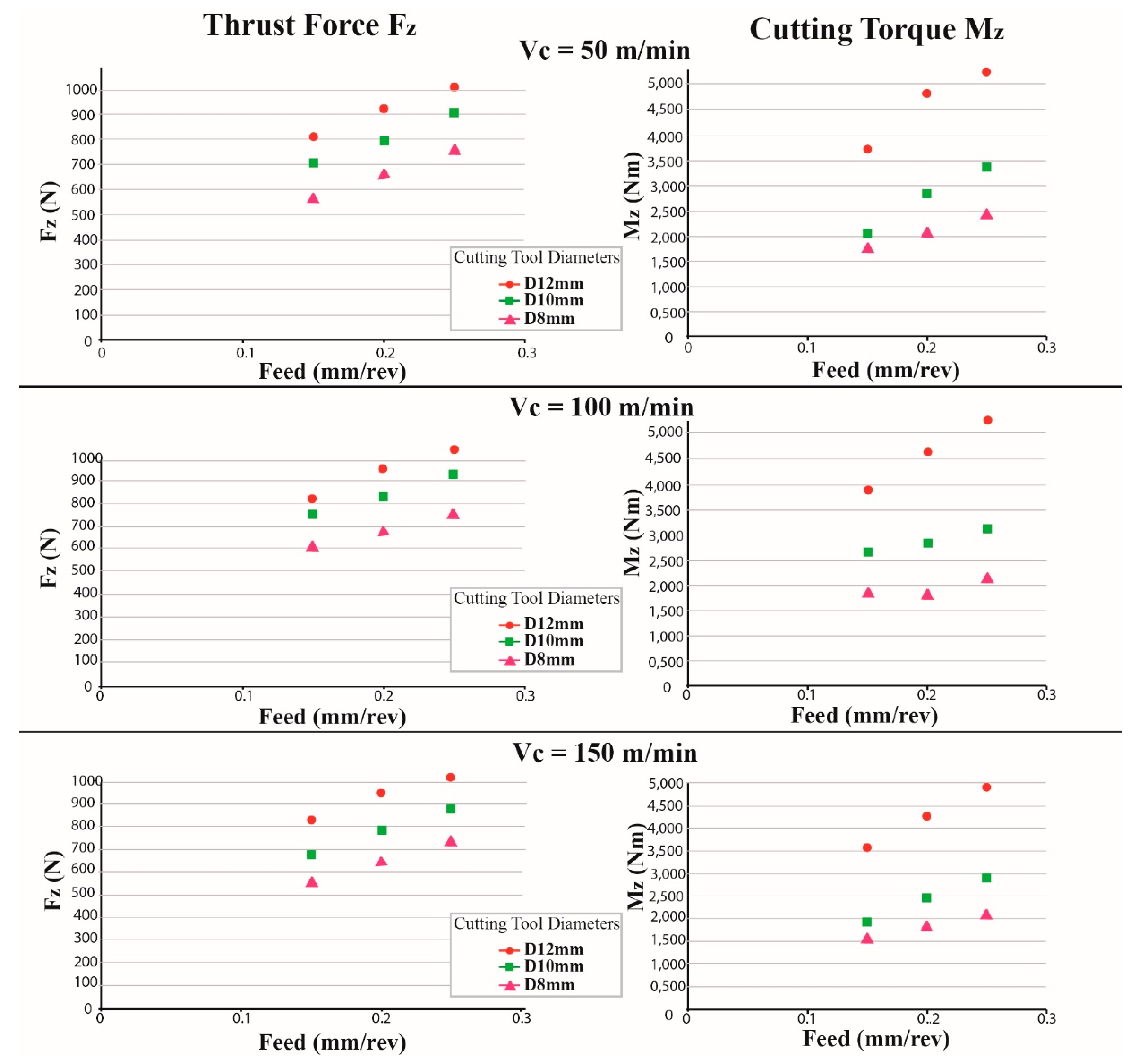
3] conducted a study on chip morphology during high speed drilling of Al-Si alloy. More specifically, they investigated the effect of cutting speed and feed rate on chip morphology by conducting observations at various surfaces of the chip using microscopy techniques. For the drilling experiments, uncoated WC drills were employed to produce 15 mm-diameter holes under various cutting speeds and feed values, in the range of 240–320 m/min and 0.16–0.24 mm/rev, respectively. It was found that, on the free surface of the chip, lamella structures were created and that an increase of speed and feed rate led to a decrease of the frequency of the appearance of these lamella structures. Regarding chip morphology, the increase of cutting speed and feed led to the increase of chip pitch and height and a decrease of the chip compression ratio. Finally, thrust force was found to increase with a decrease of cutting speed and an increase of the feed rate, so it was suggested that high cutting speeds are essential in order to minimize thrust force in the case of Al-Si alloys’ drilling.
Qiu et al. [4] investigated the use of high-performance drills during drilling of aluminum and titanium alloys with a view toward minimizing cutting force and torque. For their experiments, they employed two conventional and two modified types of drills, which had larger point, primary relief, and helix angles and a lower second clearance angle. For the aluminum alloy, the cutting speed was varied from 100–200 m/min and the feed rate from 0.1–0.2 mm/rev. The experiments indicated that the tools with the modified geometry were able to reduce thrust force and torque in the majority of cases, with the average reduction of force being 9.78% and torque 21.08%. Dasch et al. [5] conducted a thorough comparison regarding various categories of coated cutting tools for the drilling process of aluminum. For their study, they used five different types of coating materials, namely carbon, graphitic, hydrogenated and hydrogen-free diamond-like carbon, and diamond on two types of drills, namely HSS and carbide drills. In the tests, they measured tool wear, temperature, and spindle power. After conducting tests on various cases of cutting speed and feed combinations, they concluded that the most important is to coat the flutes of the tool rather than the cutting edge, that coated tools were able to drill up to 100-times more holes than the uncoated, and that hydrogenated carbon coatings are superior to the other types of coating.
Regarding modeling of the drilling process, various studies have been conducted due to its popularity. Kurt, Bagci, and Kaynak [6] determined the optimum cutting parameters for high surface quality and hole accuracy using the Taguchi method. In their work, they conducted experiments at various cutting speeds, feed rates, and depths of drilling and tested the performance of both uncoated and coated HSS drills. After the experiments were conducted by the Taguchi method, regression models for Ra, and hole diameter accuracy were derived, and the optimum parameters were identified by analyzing the S/N ratio results. Kilickap [7] used the Taguchi method and Response Surface Methodology (RSM) to predict burr height during drilling of aluminum alloys and to determine the optimum drilling parameters. He conducted experiments using various cutting speeds, feed rates, and point angles and observed the burr height and surface roughness. Analysis using the Taguchi method and Analysis Of Variance (ANOVA) revealed the optimum parameters for reducing the burr height and surface roughness, and regression models created using RSM were proven to be adequate to describe the correlation between process parameters and process outcome. Sreenivasulu and Rao [8], Efkolidis et al [9], and Kyratsis et al [10] also employed the Taguchi method to determine the optimum levels of the process parameters for the minimization of thrust force and torque during drilling of aluminum alloys. After they performed experiments at various cutting speeds, feed rates, and various drill diameters and geometries, they determined the most significant parameters of the process and their optimum values.
Apart from regression models, several studies based on neural network models have been reported in the relevant literature. Singh et al. [11] employed an Artificial Neural Network (ANN) model to predict tool wear during drilling of copper workpieces. As inputs for the neural network, feed rate, spindle speed, and drill diameter were selected, and thrust force, torque, and maximum wear were the outputs. After the optimum number of hidden layers and neurons, as well as the optimum learning rate and momentum coefficient were determined, it was shown that the best neural network predicted tool wear with a maximum error of 7.5%. Umesh Gowda et al. [12] presented an ANN model for the prediction of circularity, cylindricity, and surface roughness when drilling aluminum-based composites. After the experiments, tool wear, surface roughness, circularity, and cylindricity were obtained as a function of machining time, and NN models were used to correlate process parameters with these quantities.
Besides the usual MLP models, other similar approaches such as RBF-NN or hybrid approaches combining MLP with fuzzy logic or genetic algorithms have also been presented. Neto et al. [13] also presented MLP and ANFIS models for the prediction of hole diameter during drilling of various alloys. For the neural network models, inputs from various sensors such as acoustic emission, electric power, force, and vibration were employed. Thorough analysis of the predicted results’ errors revealed that MLP models had superior performance to ANFIS models. Ferreiro et al. [14] conducted a comprehensive study in developing an AI-based burr detection system for the drilling process of Al7075-T6. For that reason, they employed data-mining techniques and tested various approaches with a view toward reducing the classification errors. All developed models performed better than the existing mathematical model for burr prediction, and in particular, it was shown that a model based on the naive Bayes method exhibited the maximum accuracy.
Lo [15] employed an ANFIS model for the prediction of surface roughness in end milling. In their models, they employed both a triangular and trapezoidal membership function with 48 sets of data for training and 24 for testing. The error was found to be minimum using the triangular membership function. Zuperl et al. [16] used an ANFIS model for the estimation of flank wear during milling. The model was trained with 140 sets of data (75 for training and 65 for testing) and included 32 fuzzy rules. It was shown that a model with a triangular membership function was again capable of exhibiting the lowest error. Song and Baseri [17] applied the ANFIS model for the selection of drilling parameters in order to reduce burr size and improve surface quality. In this work, a different model was built for each of the four outputs, namely burr height, thickness, type, and hole overcut. One hundred and fifty datasets were used, 92 for the training, 25 for checking, and 25 for testing of the model. For the first output, the best model had four membership functions of a triangular type; for the second one, the best model had a three-membership function of a Gaussian type; and the last two three- and four-membership functions of a generalized bell type, respectively. Fang et al. [18] used an RBF model for surface roughness during machining of aluminum alloys. Their model included eight inputs, related to process parameters, cutting forces, and vibration components, and five outputs, related to surface roughness. The RBF model was proven to be faster than an MLP model, but it was inferior in terms of accuracy. Elmounayri et al. [19] employed an RBF model for the prediction of cutting forces during ball-end milling. The model had four inputs, related to the process parameters and four outputs, namely the maximum, minimum, mean, and standard deviation of instantaneous cutting force. In this case, it was noted that the RBF network was more efficient and accurate and faster than the classical MLP.
Although comparisons between regression models and neural network model for cases of machining processes have already been conducted, comparison between several soft computing methods has rarely been conducted, and only a few relevant studies exist. Tsai and Wang [20] conducted a thorough comparison between various neural network models such as different variants of MLP, RBF-NN, and ANFIS for the cases of electrical discharge machining. They concluded that the best performing method was ANFIS, as it exhibited the best accuracy among the tested methods. Nalbant et al. [21] conducted a comparison between regression and artificial neural network models for CNC turning cases and concluded that although the neural network model was performing slightly better, both models were appropriate for modeling the experimental results. Jurkovic et al. [22] compared support vector regression, polynomial regression, and artificial neural networks in the case of high-speed turning. Their models included feed, cutting speed, and depth of cut as inputs, and separate models were created for three output quantities, namely cutting forces, surface roughness, and cutting tool life. In the cases of cutting force and surface roughness, they found that the polynomial regression model was the best, whereas in the case of cutting tool life, ANN performed better than the other methods.
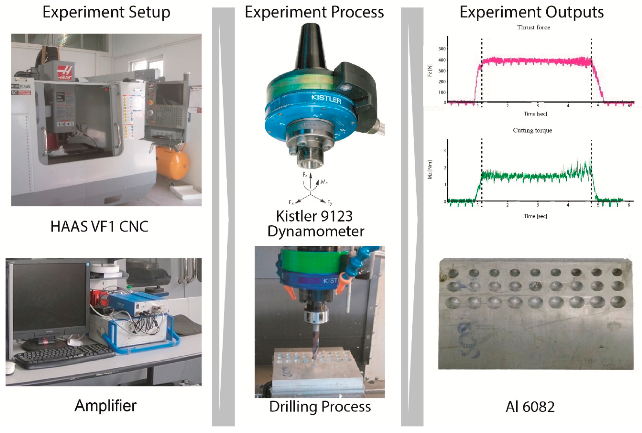
In the present study, a comparison of various neural network models, as well as multiple regression models is conducted with a view toward determining the best performing model for the case of drilling Al6082-T6. As in this case, a relatively small dataset is used, it is expected that the results of regression models and neural network models will be comparable, and so, it is interesting to find out whether there can be a clear difference in the performance of these methods in the present case. The various neural network models are trained with different parameters, and the comparison between them is conducted by criteria relevant to the prediction error, both for training and testing datasets.

2. Artificial Neural Networks

Artificial neural networks are among the most important soft computing methods, widely used for a great range of applications spanning across various scientific fields. This method is able to successfully predict the outcome of a process by using pairs of input and output data in a learning procedure. In fact, this method imitates the function of biological neurons, which receive inputs, process them, and generate a suitable output. The most common ANN model, namely MLP, has a structure containing various interconnected layers of neurons, starting from an input layer and ending at an output layer. The middle layers are called hidden layers, and their number is variable, depending on the size and the characteristics of each problem. Each neuron is connected by artificial synapses to the neurons of the following layer, and a weighting coefficient, or weight, is assigned to each synapse. The inputs for each neuron are multiplied by the weighting coefficient of the respective synapse, and then, they are summed; after that, the output from each neuron is generated by using an activation function, which usually is a sigmoid function, such as the hyperbolic tangent.
The ANN model is created by a learning process, containing three different stages, i.e., training, validation, and testing. For each stage, a part of the total input/output data is reserved, most commonly 70%, 15%, and 15%, respectively. The learning process consists of the determination of suitable weight values according to real input/output data pairs and is an iterative process. This process is called error backpropagation, as the difference of the predicted and actual output is first computed in the output layer, and then, the error is propagated through the network in the opposite way, from the output to the input layer; after various iterations, or epochs, the network weights are properly adjusted so that the error is minimized. The training and validation stage both involve adjustment of the weights, and it is possible to stop the learning process if the error is not decreasing after some epochs, a technique that is named the early stopping technique. Finally, during the testing stage, the trained model is checked for its generalization capabilities by providing it with unknown data from the testing data sample. Usually, the Mean Squared Error (MSE) is used for the determination of model performance:
M S E = 1 n i = 1 n ( Y i A i ) 2
where n is the number of data samples, Yi are the predicted values and Ai the actual values.
Furthermore, the Mean Absolute Percentage Error (MAPE) can be also employed to evaluate the results of neural network models:
M A P E = 100 % n i = 1 n | Y i A i A i |
Finally, RBF-NN is constructed by using an appropriate radial function as the activation function for a neural network model with a single layer. Most commonly, a Gaussian-type function is used as the activation function:
φ ( r ) = e ε r 2
where ε is a small number and r = x x i , with x being an input and xi the center of the radial basis function. Apart from the widely-used MLP model and RBF-NN models, various other types of neural networks exist, as well as hybrid models, combining ANN with other soft computing methods such as fuzzy logic. In addition to the learning and optimization ability of the neural networks, fuzzy logic systems are able to provide a means for reasoning to the system with the use of IF-THEN rules. ANFIS is a soft computing method with characteristics related both to neural networks and fuzzy logic. Generally, the creation of an ANFIS model has several similarities to the creation of a MLP model, but there exist also some basic differences. This model has a structure similar to the MLP structure, but there are some additional layers, related to membership functions of the Fuzzy Inference System (FIS). One of the most common fuzzy models used in ANFIS models is the Sugeno fuzzy model. By the training process, fuzzy rules are formed, and an FIS is created. At first, the input data are converted into fuzzy sets through a fuzzification layer, and then, membership functions are generated. Membership functions can have various shapes such as triangular, trapezoid, or Gaussian, among others. In the second layer, the number of nodes is equal to the number of fuzzy rules of the system; the determination of the number of fuzzy rules is conducted using a suitable method such as the subtractive clustering method. The output of the second layer nodes is the product of the input signals, which they receive from the previous nodes. Then, in the third layer, the ratio of each rule’s firing strength to the sum of the firing strengths of all rules is calculated, and it is used in the defuzzification layer to determine the output values from each node. Finally, the total output is calculated by summation of the outputs of the fourth layer. The FIS parameters are updated by means of a learning algorithm in order to reduce the prediction error, such as in the case of MLP model.

3. Methods and Materials

3.1. Technics of Experiments

In the present work, it is intended to conduct a comparison of various methods, which can be employed for modeling of the drilling process of Al6082-T6. The datasets for the models were obtained by conducting experiments on an Al6082-T6 workpiece. This work material used for the present investigation was a 140 mm × 100 mm × 30 mm plate with the chemical composition and main mechanical properties as summarized in Table 1.
Drilling experiments were carried out on a HAAS VF1 CNC machining center using solid carbide drill tools. Two components of drilling loads (thrust force Fz and torque Mz values) were recorded with a Kistler dynamometer Type 9123 connected to a three-channel charge amplifier with a data acquisition system. Dynoware software (Type 2825D-02) was used in order to monitor and record the experimental values of the cutting forces, as shown in Figure 1.

3.2. Methodology of Results Analysis

The experiments were conducted according to a full factorial strategy. The three cutting parameters selected for the present investigation were the cutting speed (V), the feed rate (f), and the cutting tool diameter (D). Cutting velocity values of 50 m/min, 100 m/min, and 150 m/min together with feed rates of 0.15 mm/rev, 0.2 mm/rev, and 0.25 mm/rev were used in combination with three cutting tool diameters (D) of 8 mm, 10 mm, and 12 mm. The constant depth of the holes drilled was 30 mm. The machining parameters used and their levels are shown in Table 2.
During the experimental process, 27 different solid carbide drilling tools (one tool for each hole) were clamped to a Weldon clamping device with a high rigidity, while a mechanical vise was used for clamping the workpiece. As the type of cutting tools (KENNAMETAL B041A/KC7325) is non-through coolant solid carbide, the cutting fluid used (KOOLRite 2270) was provided by the delivery system near them. Figure 2 demonstrates all the dimensional details of the main shape of the cutting tools. All the possible combinations of the manufacturing parameters were used (cutting speed, feed rate, tool diameter).
As shown in Figure 3, apart from multiple regression method, three soft computing methods, related to artificial neural networks, namely MLP, RBF-NN, and ANFIS methods, were used.
For the development of the model, MATLABTM software was employed. For each method, only one characteristic, mainly related to the architecture of the network, was varied, and the other settings were assumed to be equal to the default settings of the software. For the MLP and RBF-NN, the number of hidden neurons was varied, and for the ANFIS, where the number of inner nodes cannot be altered in the same way as in the other two types of networks, the number of clusters used for the data, using the fuzzy c-means clustering method, which directly affects the number of parameters of the system, was varied. In all cases, the lower and upper boundaries for the variable parameters were chosen in a way that it did not lead to extreme overfitting; the analysis conducted was able to determine exactly the limit values of the variable parameters, which can lead to a properly-functioning model.
The choice of the number of hidden neurons is crucial in the case of MLP and RBF-NN, as it can increase the accuracy of the network up to a point, and then, it causes problems of overfitting. In the relevant literature, no certain methodology for the determination of the exact number of hidden neurons exists; there are several empirical rules, which usually relate the appropriate number of hidden neurons with the number of input and output variables. However, the number of available pairs of input/output data also affects the choice of the number of hidden neurons, as it is not appropriate to use more network parameters, e.g., weights and biases, than the number of available input/output data pairs. This is especially important for the present study, as the size of dataset was relatively small, namely 27 input/output data pairs. For the determination of the lower and upper value of the number of hidden neurons, in order not to conduct an exhaustive search, the recommendations from some empirical relationships were taken into consideration. In [23], it was proposed that the number of hidden neurons could be approximated as follows:
n = N i n p + N o u t + a
where Ninp is the number of input neurons, Nout the number of output neurons, and α is a number between zero and 10. In the present case, Ninp equals to three, i.e., drill diameter, cutting speed, and feed, and Nout is one, i.e., thrust force or cutting torque. Thus, according to this formula, the lower and upper boundaries for the number of hidden neurons in the present study was between two and 12. However, in the present study, an investigation of the optimum value of hidden neurons was conducted by taking into consideration the performance of the models regarding not only MSE, but also MAPE, both for the training and testing dataset, as it is required to achieve a low value of error for the training data, but also to prevent the network from overfitting, something that is indicated by the error in the testing dataset. For the MLP and RBF-NN, the number of hidden neurons is varied between one and eight, a choice that is comparable to the suggestions offered by Equation (4). Each network was trained 50 times with the same settings in order to overcome the effect of the random initialization of weights. For the ANFIS models, the parameter that was varied was the number of clusters, in the range of 2–4. As with the other two types of networks, the training was repeated 50 times, and the results regarding MSE and MAPE for training and testing data are presented.
For all models, the data pairs reserved for the testing stage of the network assessment were selected randomly, but were the same in order to conduct a more appropriate comparison between these models. Models were developed separately for thrust force Fz and torque Mz. In Figure 4, a flowchart presenting graphically the procedure followed in the present study is depicted.

4. Results and Discussion

4.1. Result of Experiment

Figure 5 shows the experimental values derived from the whole process. It is clear that there was a relationship between cutting parameters and cutting forces. When the tool diameter increased, both cutting forces increased. As the feed rate values increased, the cutting forces increased respectively. The cutting speed did not noticeably affect either cutting force. A full factorial strategy was applied, and twenty seven (27) drilling experiments were performed, while both Fz and Mz were modelled separately using polynomial mathematical models.

4.2. Multiple Regression Models

The RSM is a tool based on the collection of statistical and mathematical techniques used for process optimization. Optimization can be managed by creating an empirical relationship between independent variables and the response of the system using the quantitative data collected from experiment [5,6]. The experiments were designed and executed by employing second-order nonlinear mathematical models in order to predict the thrust force and the cutting torque, which are of the following form:
Y = b 0 + b 1 X 1 + b 2 X 2 + b 3 X 3 + b 4 X 1 2 + b 5 X 2 2 + b 6 X 3 2 + b 7 X 1 X 2 + b 8 X 1 X 3 + b 9 X 2 X 3
where Y is the response, Xi stands for the coded values, and bi stand for the models’ regression coefficients.
When the level of significance is very small, less than 0.05, this indicates that the results were high and probably not randomly scattered. The significant terms were found by Analysis Of Variance (ANOVA) for each response (Table 3 and Table 4).
The following regression equations for the thrust force and the cutting torque as a function of three input process variables were developed:
F z =     222   +   57.6   D   +   1.96   V   +   1292   f     0.76   D * D     0.0117   V * V     667   f * f +   0.0560   D * V   +   103   D * f     1.20   V * f  
and:
M z =   12.9     2.67   D   +   0.0137   V     15.6   f   +   0.140   D * D     0.000055   V * V   +   4.7   f * f           0.000122   D * V   +   2.63   D * f     0.0233   V * f
where D is the tool diameter (mm), f is the feed rate (mm/rev), and V is the cutting speed (m/min).
The p-values are used as a basic tool to check the importance of each of the coefficients. The smaller the amount of P, the more significant is the corresponding coefficient. In our case, for Fz, these factors are: D (p-value = 0.026), V (p-value = 0.002), V*V (p-value = 0.000), and D*f (p-value = 0.005), while for Mz, the significant terms are: D (p-value = 0.000), D*D (p-value = 0.000), V*V (p-value =0.046), and D*f (p-value = 0.000). Moreover, from Table 3 and Table 4, it is evaluated that the coefficient of multiple determination was very close to unity for both cases (R2 = 99.6% for Fz and R2 = 98.9% for Mz), and the adjusted coefficient (R2 adj) was 99.4% for Fz and 98.3% for Mz. All these statistical estimators indicate an appropriate RSM model with the degree of freedom and optimal architecture that can be used for predictive simulations of the reactive extraction. Of course, for both cases, only the significant terms can be included in order to present a set of simplified equations. The agreement between experimental and RSM predicted data is shown in Figure 6. Residual analysis was performed to test the models’ accuracy; in both cases, all points were positioned near to a straight line, indicating that RSM predicts the experimental data for the considered valid region well.

4.3. Multi-Layer Perceptron Models

As was described in the Methods and Materials section, in the case of MLP models, an investigation of the optimum number of hidden neurons was conducted based on various criteria. After the MLP models were developed, the results obtained were as presented in Table 5.
As can be seen from Table 5 and Figure 7, in the case of the thrust force model, the MSE for the training dataset was generally decreasing with an increase of the number of hidden neurons. Especially, for models with over five neurons, the MSE became extremely small, indicating that the training dataset can be reproduced with a high level of accuracy by this model. However, the MSE for the testing dataset, which is an indication of overfitting, became the minimum for the model with four hidden neurons and then increased again. A similar situation was observed in the case of MAPE, where MAPE for the training dataset became extremely small for networks with more than four hidden neurons, but the minimum MAPE for the testing dataset was obtained for the model with five hidden neurons. Thus, the optimum number of hidden neurons was four or five, and the final choice was conducted in terms of total error, as the error values for these cases were very close. Finally, the case with four neurons was chosen as the total error was very close to the total error of the case with five neurons, and this network was less complex than the other.
As can be seen from Table 6 and Figure 8, in the case of the torque model, the MSE for training was decreasing with an increasing number of hidden neurons, mainly for models with more than six hidden neurons. However, the minimum value of MSE for the testing dataset was obtained for the model with four hidden neurons. Regarding MAPE, the minimum value for the training dataset was obtained for the model with seven hidden neurons, whereas the minimum value for the testing dataset was obtained for the model with six hidden neurons. Thus, the best model was determined again by checking the total error, and it was determined that the network with six hidden neurons was the best performing one. Generally, it was observed that the error values for the Mz model were considerably larger than those of the Fz model. Nevertheless, the results confirmed that the optimum number of neurons was dependent on the size of the dataset; as for the relatively small dataset of 27 samples, a model with six hidden neurons was sufficient.

4.4. Radial Basis Function Neural Network Models

As was previously mentioned, in the case of RBF-NN models, it is intended to determine the optimum number of hidden neurons. In Table 3, the results from the RBF-NN models are presented.
For the RBF-NN models in the case of thrust force, it can be observed from Table 7 and Figure 9 that MSE for the training set was decreasing with an increasing number of hidden neurons, but there was not such a large decrease as in the case of MLP models. For the testing dataset, MSE was the minimum for the model with seven hidden neurons, and the same was noted for MAPE for the training dataset. Thus, the model with seven hidden neurons was the optimum in this case. It is to be noted that the value of MAPE for both the training and testing dataset was considerably reduced for models with over three neurons, something that was not observed to a similar extent in the case of MLP models, at least for the testing dataset.
As for the torque (Mz) cases, it was observed from Table 8 and Figure 10 that the optimum model was the one with eight hidden neurons, as it exhibited both a lower MSE and MAPE for the testing dataset. Thus, it can be stated that for RBF-NN models, a slightly larger number of hidden neurons was required compared to MLP models.

4.5. Adaptive Neuro-Fuzzy Inference System Models

In the case of ANFIS models, results from cases with a different number of clusters are presented in Table 9.
In the case of the ANFIS models for thrust force, it can be seen from Table 9 and Figure 11 that the MSE for both training and testing datasets was reduced with an increasing number of clusters. Furthermore, the same can be observed for the MAPE for both datasets; thus, the ANFIS model with four clusters was selected as the best performing network. In the case of torque models, whose results are presented in Table 10 and Figure 12, the optimum value of MSE for the testing dataset was obtained for the model with two clusters, whereas the optimum value of MAPE for the testing dataset was obtained for the model with four clusters. Therefore, the best model was selected according to the total error values, which were lower for the model with four clusters.

4.6. Comparison of Regression and Neural Network Models

The thrust force and cutting torque predictive models were developed by RSM and ANN by implementing a full factorial experimentation design depending on the effects of the selected cutting parameters such as cutting speed, feed rate, and tool diameter. Figure 13 and Figure 14 illustrate the comparison between the experimental values of Fz and Mz and their values of the ANN and RSM models, respectively.
After the results regarding all developed models were presented, a comparison between these models was conducted. For the comparison, the best model from each method was selected, and its performance was evaluated using the same criteria, as can be seen in Table 11. As for the regression model, the MSE was not calculated, and also, no separate dataset for training and testing exists, so the total MAPE for each case was chosen as the criterion for the comparison between all models.
Among the three neural network models, it can be seen that the MLP model had the lowest MAPE values in all cases, followed by the ANFIS model and the RBF model. The MLP and ANFIS models were clearly superior to the RBF model and also better than the regression model. Thus, it can be concluded that the MLP model was more appropriate for the modeling of thrust force and torque in the presented case. Finally, given the relatively small size of the neural networks model, there was no significant difference in terms of computational time between these approaches and the regression model, and so, it was shown that these models can perform efficiently for the presented case.

5. Conclusions

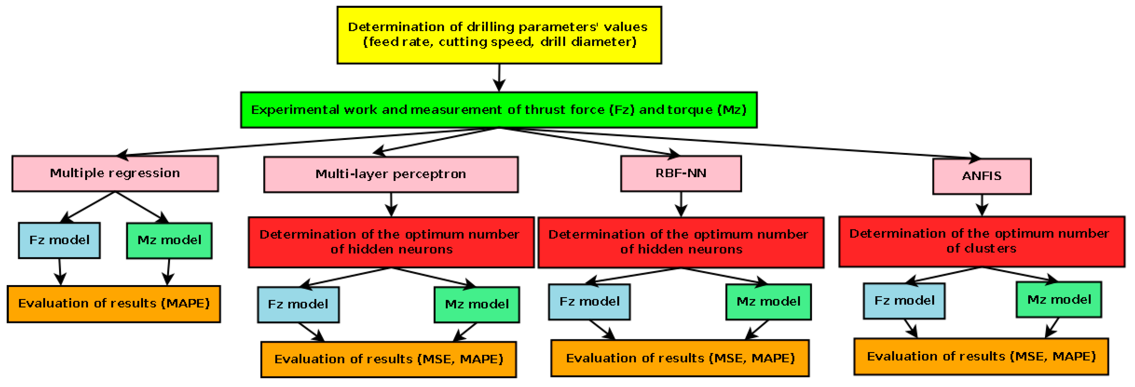
In the present paper, various methods for the modeling of the drilling process, such as regression and neural network models, were compared in order to determine which is the most accurate and efficient one. These models were applied to cases of drilling Al 6082-T6 alloy under various process conditions. From this study, several conclusions can be drawn.
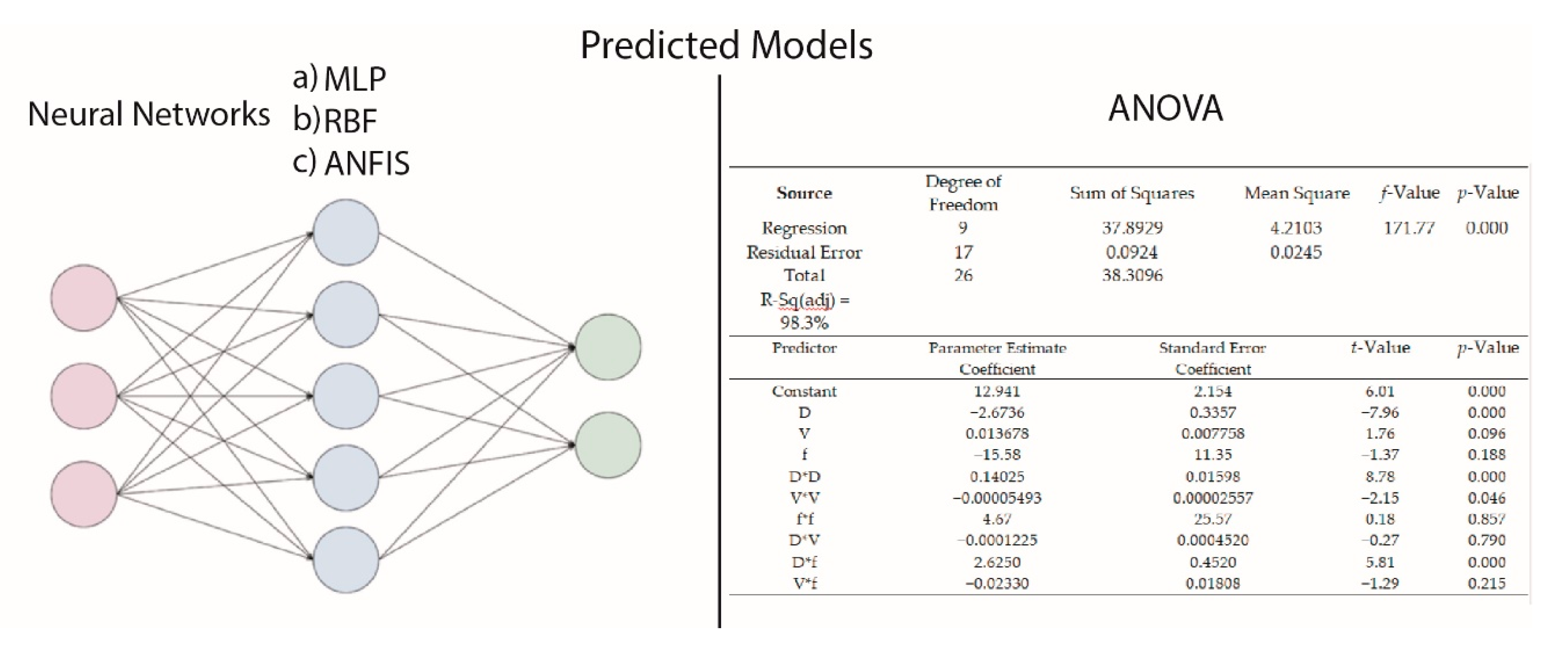
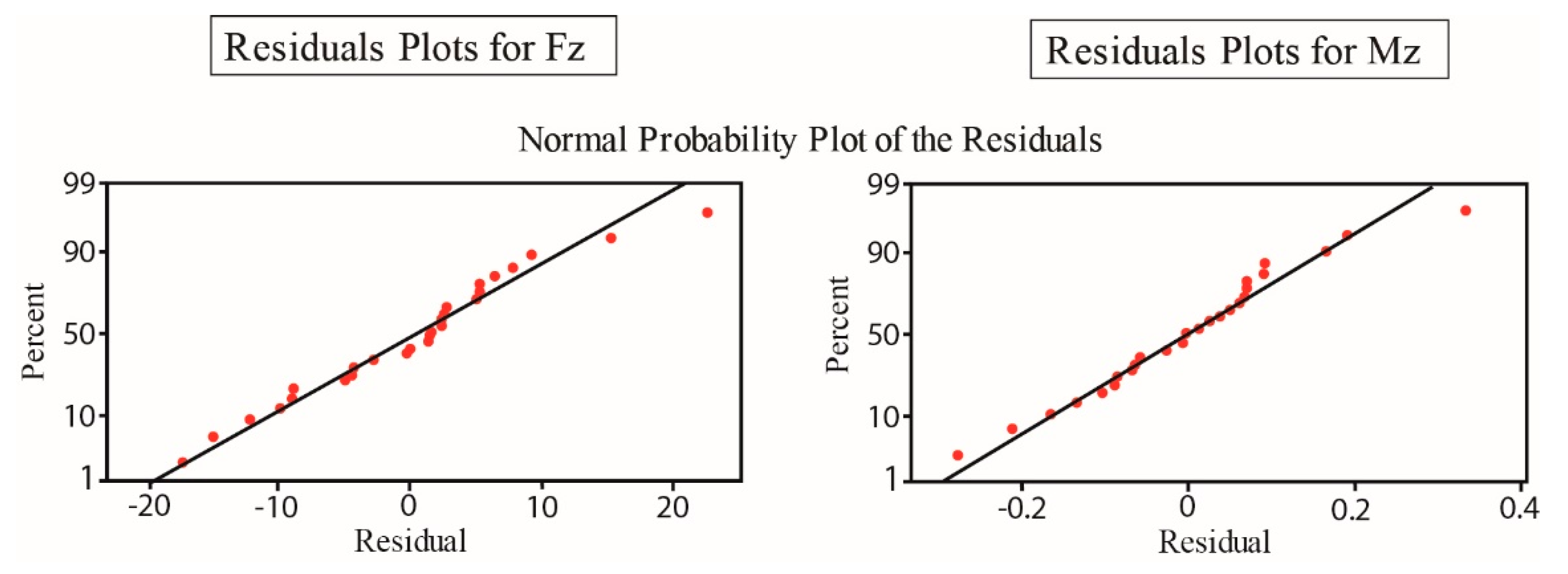
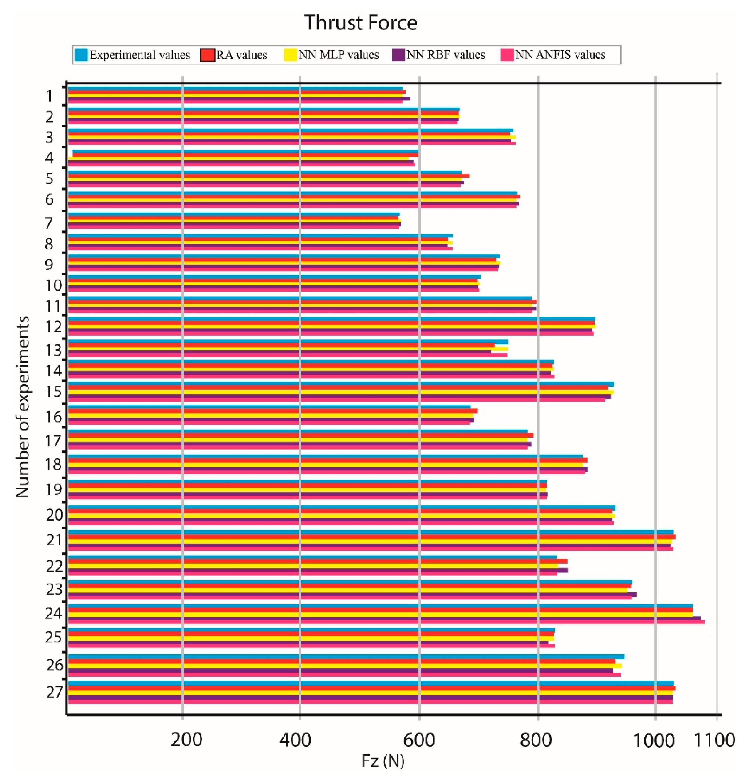
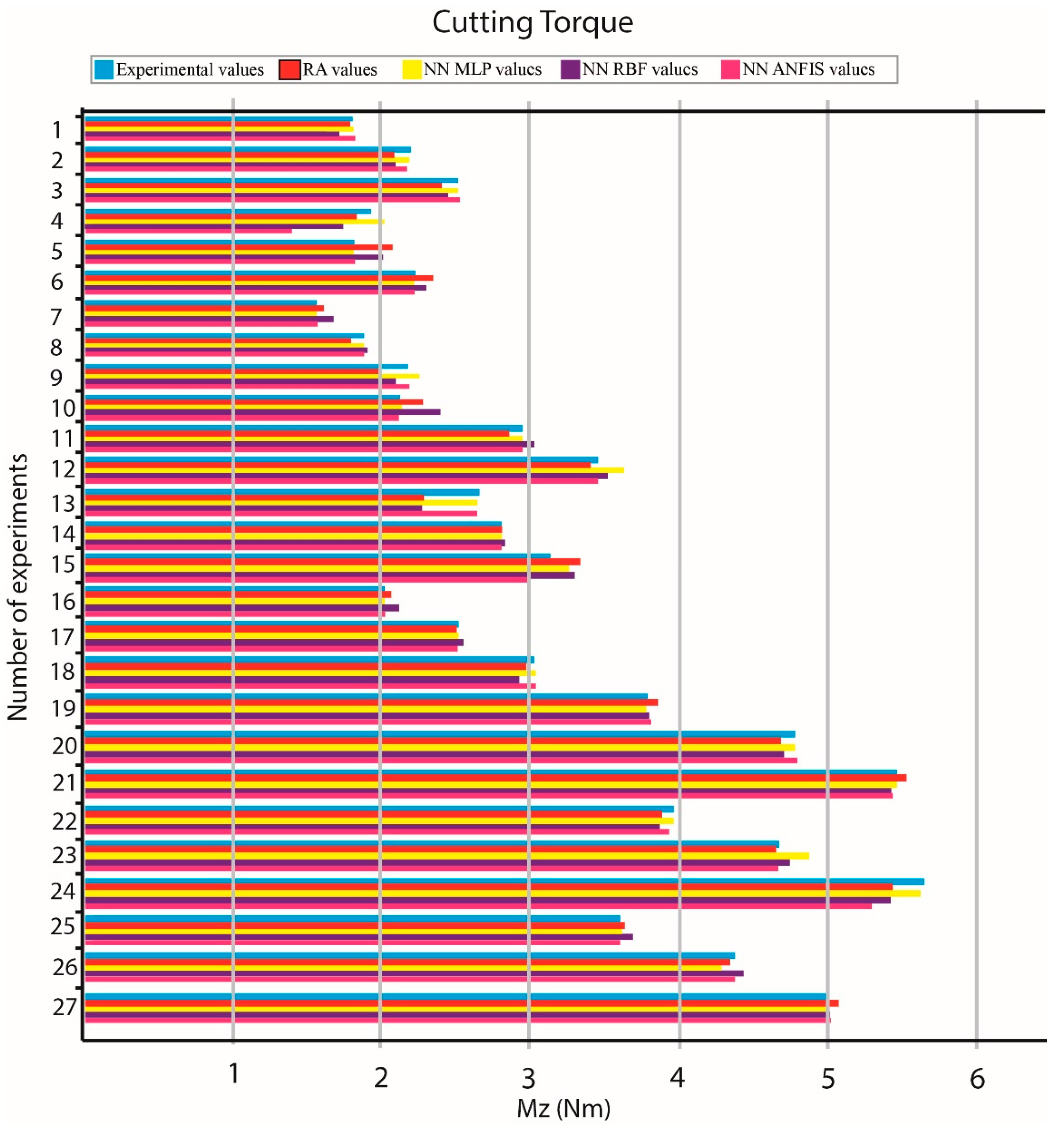
From the statistical analysis and derivation of the multiple regression models, it can be deduced that the developed models are sufficiently accurate, as they exhibited high correlation coefficient values, namely 99.6% and 98.9% for the Fz and Mz models, respectively, and also low MAPE values, namely 0.86305% and 3.0495% for the Fz and Mz models, respectively.
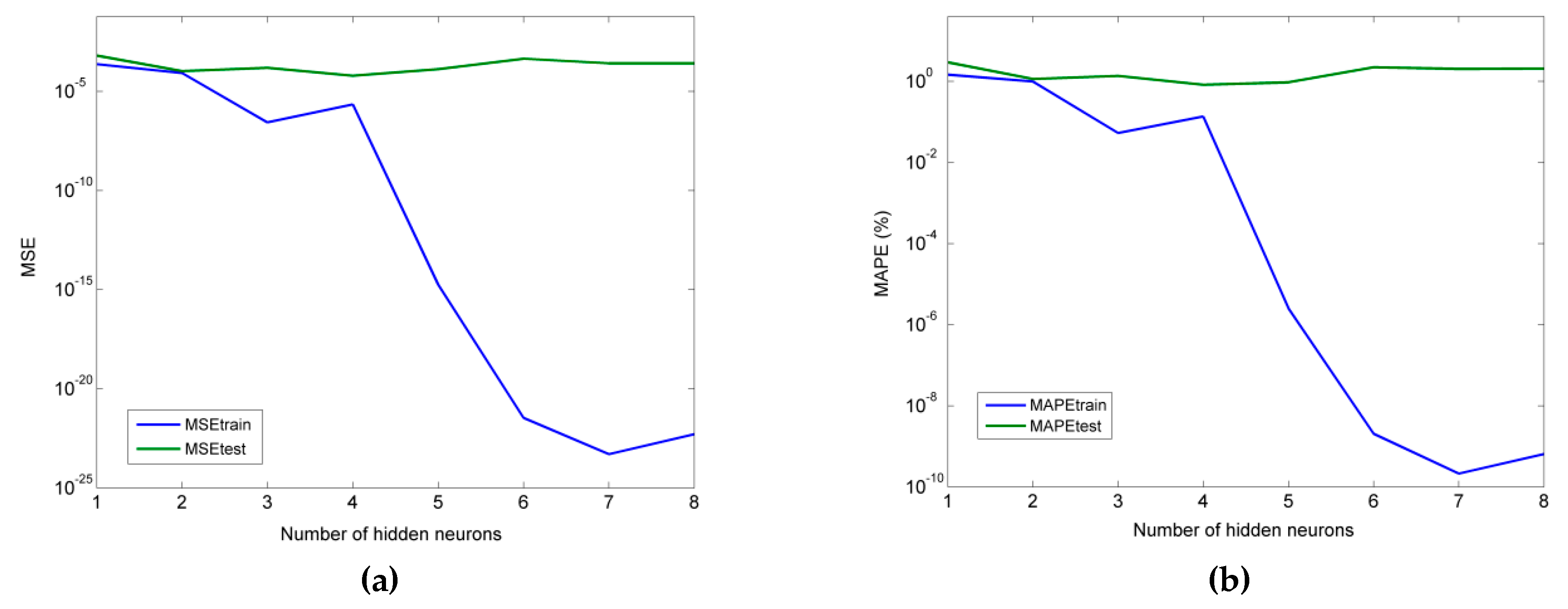
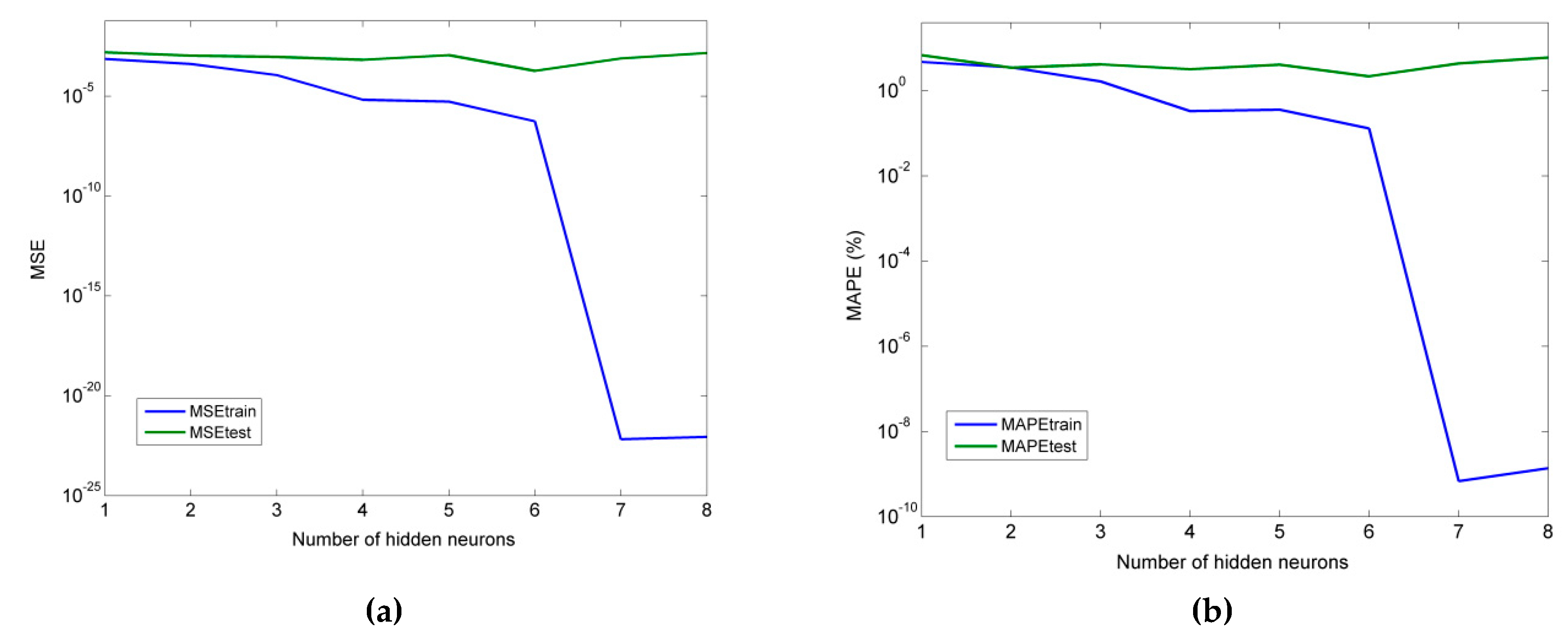
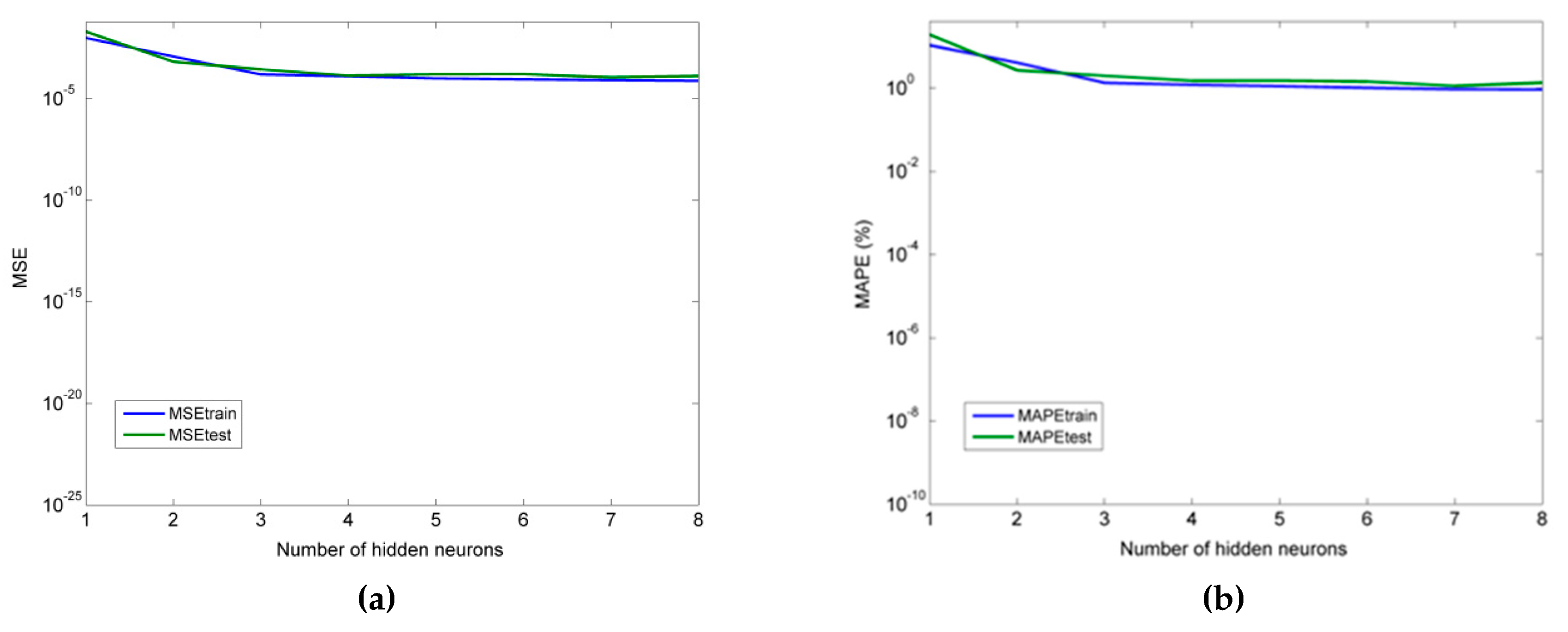
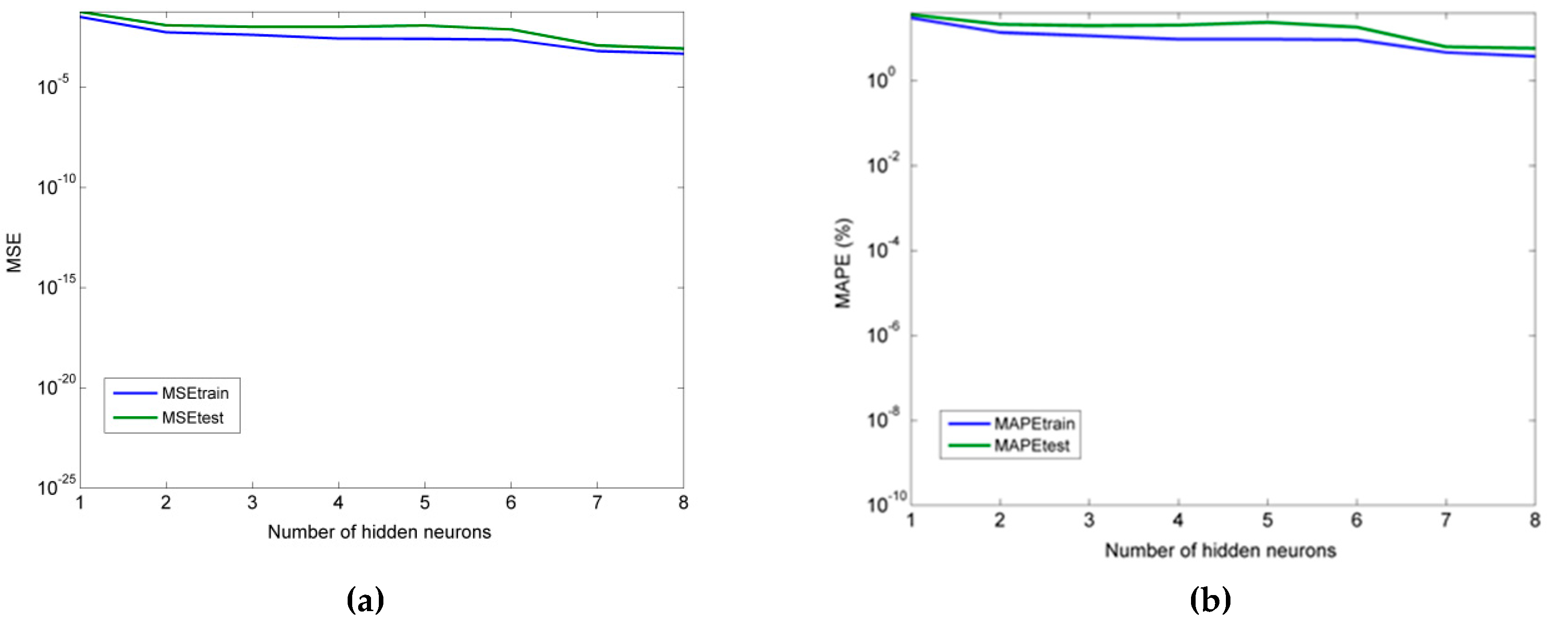
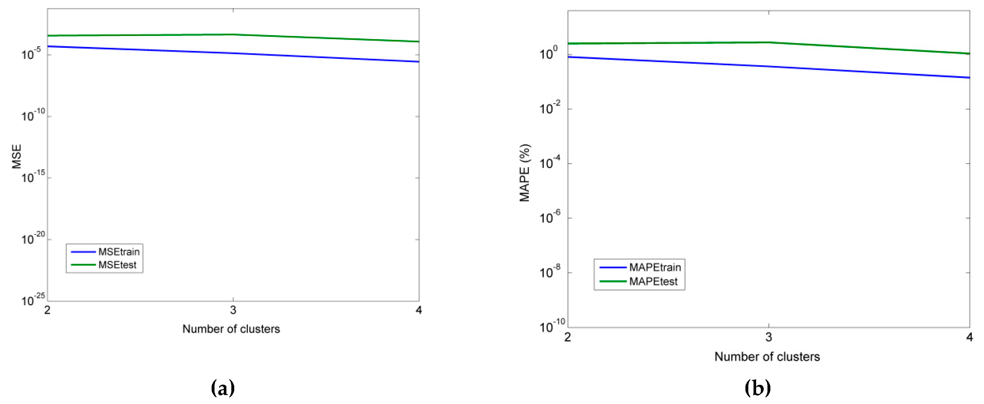
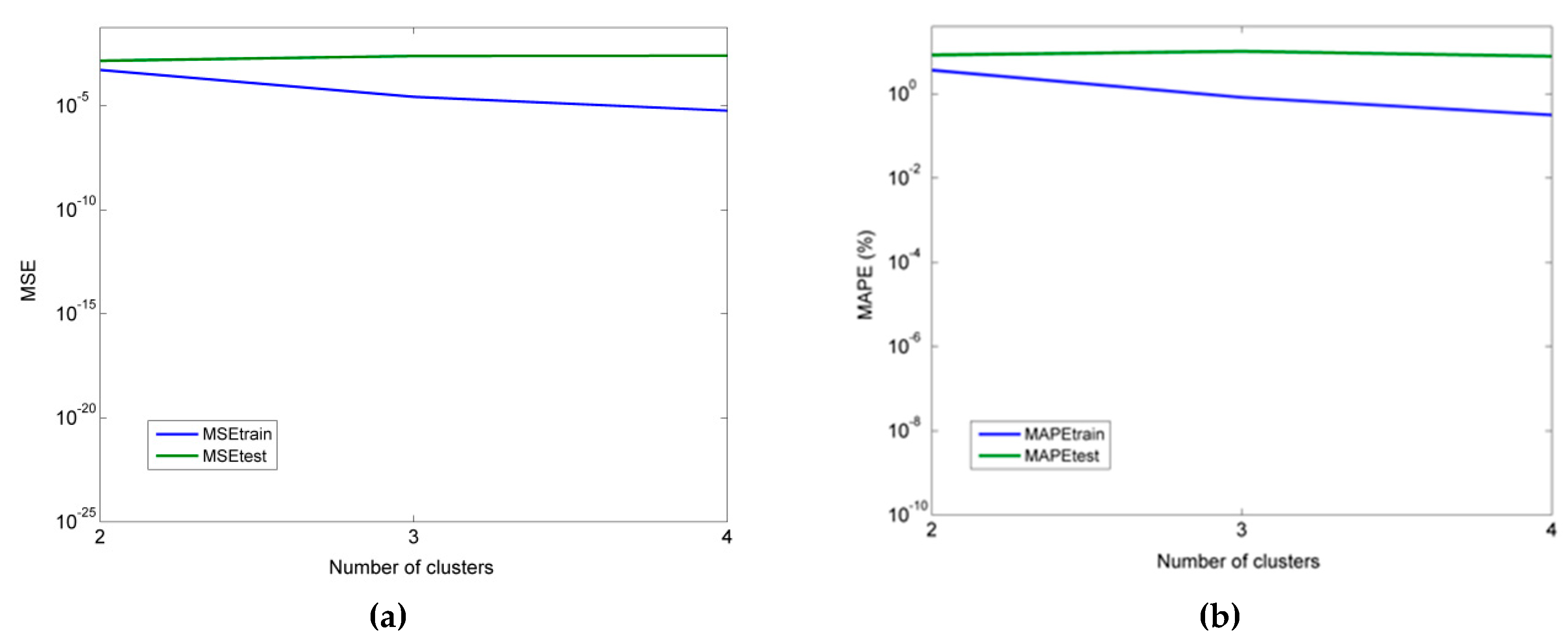
As for the neural network models, it was determined that an MLP model with 4 hidden neurons was more suitable for the prediction of thrust force, and an MLP model with six hidden neurons was more appropriate for the prediction of cutting torque. Furthermore, for the RBF-NN model, a higher number of hidden neurons was shown to lead to better accuracy, namely seven and eight in the cases of thrust force and torque, respectively. Finally, for the ANFIS models with fuzzy c-means clustering, the use of four clusters was the best choice in both the Fz and Mz cases.
From the comparison of all models, it was concluded that the MLP model performed better in all cases, followed by ANFIS, multiple regression, and RBF-NN. Thus, it was shown that MLP can be competitive with multiple regression models even for relatively small datasets and that ANFIS and RBF-NN are less suitable for cases with small datasets.

Author Contributions

Conceptualization, N.E.K., N.E., P.K., and A.P.M.; methodology, N.E.K., N.E., P.K., and A.P.M.; software, N.E.K. and N.E.; validation, N.E. and P.K.; formal analysis, N.E.K. and N.E.; investigation, N.E.K., N.E., P.K., and A.P.M.; resources, P.K. and A.P.M.; writing, original draft preparation, N.E.K. and N.E.; writing, review and editing, P.K. and A.P.M.; supervision, P.K. and A.P.M.

Funding

This research received no external funding.

Conflicts of Interest

The authors declare no conflict of interest.

References

  1. Nouari, M.; List, G.; Girot, F.; Gehin, D. Effect of machining parameters and coating on wear mechanisms in dry drilling of aluminum alloys. Int. J. Mach. Tools Manuf. 2005, 45, 1436–1442. [Google Scholar] [CrossRef]
  2. Girot, F.; Gutierre-Orrantia, M.E.; Calamaz, M.; Coupard, D. Modeling and adhesion tool wear in dry drilling of aluminum alloys. AIP Conf. Proc. 2011, 1315, 1639–1644. [Google Scholar]
  3. Farid, A.A.; Sharif, S.; Idris, M.H. Chip morphology study in high speed drilling of Al-Si alloy. Int. J. Adv. Manuf. Technol. 2011, 57, 555–564. [Google Scholar] [CrossRef]
  4. Qiu, K.; Qin, S.; Ge, C.; Chen, M. A study of high-performance drills in the drilling of aluminum alloy and titanium alloy. Key Eng. Mater. 2014, 589–590, 163–167. [Google Scholar] [CrossRef]
  5. Dasch, J.M.; Ang, C.C.; Wong, C.A.; Cheng, Y.T.; Weiner, A.M.; Lev, L.C.; Konca, E. A comparison of five categories of carbon-based tool coatings for dry drilling of aluminum. Surf. Coat. Technol. 2006, 200, 2970–2977. [Google Scholar] [CrossRef]
  6. Kurt, M.; Kaynak, Y.; Bagci, E. Evaluation of drilled hole quality in Al2024 alloy. Int. J. Adv. Manuf. Technol. 2008, 37, 1051–1060. [Google Scholar] [CrossRef]
  7. Kilickap, E. Modeling and optimization of burr height in drilling of Al-7075 using Taguchi method and response surface methodology. Int. J. Adv. Manuf. Technol. 2010, 49, 911–923. [Google Scholar] [CrossRef]
  8. Sreenivasulu, R.; Rao, C.S. Effect of drilling parameters on thrust force and torque during drilling of aluminum 6061 alloy-based on Taguchi design of experiments. J. Mech. Eng. 2016, 46, 41–48. [Google Scholar] [CrossRef]
  9. Efkolidis, N.; Garcia-Hernandez, C.; Huertas-Talon, J.L.; Kyratsis, P. Modelling and prediction of thrust force and torque in drilling operations of Al7075 using ANN and RSM Methodologies. Strojinski Vestn. J. Mech. Eng. 2018, 64, 351–361. [Google Scholar]
  10. Kyratsis, P.; Markopoulos, A.; Efkolidis, N.; Maliagkas, V.; Kakoulis, K. Prediction of thrust force and cutting torque in drilling based on the response surface methodology. Machines 2018, 6, 24. [Google Scholar] [CrossRef]
  11. Singh, A.K.; Panda, S.S.; Pal, S.K.; Chakraborty, D. Predicting drill wear using an artificial neural network. Int. J. Adv. Manuf. Technol. 2006, 28, 456–462. [Google Scholar] [CrossRef]
  12. Umesh Gowda, B.M.; Ravindra, H.V.; Ullas, M.; Naveen Prakash, G.V.; Ugrasen, G. Estimation of circularity, cylindricity and surface roughness in drilling Al-Si3N4 metal matrix composites using artificial neural network. Procedia Mater. Sci. 2014, 6, 1780–1787. [Google Scholar] [CrossRef]
  13. Neto, F.C.; Geronimo, T.M.; Cruz, C.E.D.; Aguiar, P.R.; Bianchi, E.E.C. Neural models for predicting hole diameters in drilling processes. Procedia CIRP 2013, 12, 49–54. [Google Scholar] [CrossRef]
  14. Ferreiro, S.; Sierra, B.; Irigoien, I.; Gorritxategi, E. Data mining for quality control: Burr detection in the drilling process. Comput. Ind. Eng. 2011, 60, 801–810. [Google Scholar] [CrossRef]
  15. Lo, S.P. An adaptive-network based fuzzy inference system for prediction of workpiece surface roughness in end milling. J. Mater. Process. Technol. 2003, 142, 665–675. [Google Scholar] [CrossRef]
  16. Zuperl, U.; Cus, F.; Kiker, E. Adaptive network based inference system for estimation of flank wear in end-milling. J. Mater. Process. Technol. 2009, 209, 1504–1511. [Google Scholar]
  17. Azarrang, S.; Baseri, H. Selection of dry drilling parameters for minimal burr size and desired drilling quality. Proc. Inst. Mech. Eng. E 2017, 231, 480–489. [Google Scholar] [CrossRef]
  18. Fang, N.; Srinivasa Pai, P.; Edwards, N. Neural network modeling and prediction of surface roughness in machining aluminum alloys. J. Comput. Commun. 2016, 4, 66460. [Google Scholar] [CrossRef]
  19. El-Mounayri, H.; Briceno, J.F.; Gadallah, M. A new artificial neural network approach to modeling ball-end milling. Int. J. Adv. Manuf. Technol. 2010, 47, 527–534. [Google Scholar] [CrossRef]
  20. Tsai, K.M.; Wang, P.J. Comparisons of neural network models on material removal rate in electrical discharge machining. J. Mater. Process. Technol. 2001, 117, 111–124. [Google Scholar] [CrossRef]
  21. Nalbant, M.; Gokkaya, H.; Toktas, I. Comparison of regression and artificial neural network models for surface roughness prediction with the cutting parameters in CNC turning. Model. Simul. Eng. 2007, 2007, 92717. [Google Scholar] [CrossRef]
  22. Jurkovic, Z.; Cukor, G.; Brezocnik, M.; Brajkovic, T. A comparison of machine learning methods for cutting parameters prediction in high speed turning process. J. Intell. Manuf. 2018, 29, 1683–1693. [Google Scholar] [CrossRef]
  23. Zhang, Z.H.; Yan, D.N.; Ju, J.T.; Han, Y. Prediction of the flow stress of a high alloyed austenitic stainless steel using artificial neural network. Mater. Sci. Forum 2012, 724, 351–354. [Google Scholar] [CrossRef]
Figure 1. The workflow used for the research.
Machines 07 00013 g001
Figure 2. Cutting tool geometry details.
Machines 07 00013 g002
Figure 3. Development of the predicted models.
Machines 07 00013 g003
Figure 4. Flowchart of the procedure followed in the present research.
Machines 07 00013 g004
Figure 5. Experimental values derived from Kistler 9123.
Machines 07 00013 g005
Figure 6. Residuals analyses for Fz and Mz.
Machines 07 00013 g006
Figure 7. Results regarding the MLP model for Fz: (a) MSE for training and testing datasets, (b) MAPE for training and testing datasets.
Machines 07 00013 g007
Figure 8. Results regarding the MLP model for Mz: (a) MSE for the training and testing datasets and (b) MAPE for the training and testing datasets.
Machines 07 00013 g008
Figure 9. Results regarding the RBF-NN model for Fz: (a) MSE for training and testing datasets and (b) MAPE for training and testing datasets.
Machines 07 00013 g009
Figure 10. Results regarding the RBF model for Mz: (a) MSE for training and testing datasets and (b) MAPE for training and testing datasets.
Machines 07 00013 g010
Figure 11. Results regarding the ANFIS model for Fz: (a) MSE for training and testing datasets and (b) MAPE for training and testing datasets.
Machines 07 00013 g011
Figure 12. Results regarding the ANFIS model for Mz: (a) MSE for training and testing datasets and (b) MAPE for training and testing datasets.
Machines 07 00013 g012
Figure 13. Comparison of the experimental values with the predicted values for Fz.
Machines 07 00013 g013
Figure 14. Comparison of the experimental values with the predicted values for Mz.
Machines 07 00013 g014
Table 1. Chemical composition and mechanical properties of Al6082.
Chemical Composition
ElementsMgCuCrFeSiMnOthersAl
Percentage0.80.10.250.50.90.50.3Balance
Mechanical Properties
AlloyTemperThermal ConductivityCoefficient of Thermal ExpansionMelting
Point
Elastic ModulusElectrical Resistivity
W/m·KK−1Min
Max
GPaΩ·m
Al6082T618024 × 10−6 555
650
70 0.038 × 10⁻⁶
Table 2. Machining factors and their levels.
FactorsNotationLevels
IIIIII
Cutting speed (m/min)V50100150
Feed rate (mm/rev)f0.150.20.25
Tool diameters (mm)D81012
Table 3. ANOVA table for Fz (thrust force).
SourceDegree of FreedomSum of SquaresMean Squaref-Valuep-Value
Regression9514.67357.186471.950.000
Residual Error172060121
Total26516.733
R-Sq(adj) = 99.4%
PredictorParameter Estimate CoefficientStandard Error Coefficientt-Valuep-Value
Constant−221.9151.4−1.470.161
D57.5923.602.440.026
V1.95500.54553.580.002
f1291.8798.01.620.124
D*D−0.7621.123−0.680.506
V*V−0.0116600.001798−6.490.000
f*f−6671798−0.370.715
D*V0.056000.031781.760.096
D*f103.2531.783.250.005
V*f−1.2031.271−0.950.357
Table 4. ANOVA table for Mz (torque).
SourceDegree of FreedomSum of SquaresMean Squaref-Valuep-Value
Regression937.89294.2103171.770.000
Residual Error170.09240.0245
Total2638.3096
R-Sq(adj) = 98.3%
PredictorParameter Estimate CoefficientStandard Error Coefficientt-Valuep-Value
Constant12.9412.1546.010.000
D−2.67360.3357−7.960.000
V0.0136780.0077581.760.096
f−15.5811.35−1.370.188
D*D0.140250.015988.780.000
V*V−0.000054930.00002557−2.150.046
f*f4.6725.570.180.857
D*V−0.00012250.0004520−0.270.790
D*f2.62500.45205.810.000
V*f−0.023300.01808−1.290.215
Table 5. Results regarding the MLP models for thrust force (Fz).
No. of Hidden NeuronsMSEtrainMSEtestMAPEtrain (%)MAPEtest (%)
12.35 × 10−46.36 × 10−4 1.46 × 1002.93 × 100
28.42 × 10−51.05 × 10−4 9.84 × 10−11.14 × 100
32.72 × 10−71.53 × 10−4 5.32 × 10−21.36 × 100
42.20 × 10−66.10 × 10−5 1.36 × 10−18.23 × 10−1
51.78 × 10−151.31 × 10⁻⁴ 2.50 × 10−69.45 × 10−1
63.40 × 10−224.42 × 10⁻⁴ 2.04 × 10−92.22 × 100
74.98 × 10−242.59 × 10⁻⁴ 2.12 × 10−102.02 × 100
85.03 × 10−232.60 × 10−46.41 × 10−102.06 × 100
Table 6. Results regarding the MLP models for torque (Mz).
No. of Hidden NeuronsMSEtrainMSEtestMAPEtrain (%)MAPEtest (%)
17.39 × 10−41.57 × 10−34.75 × 1006.86 × 100
24.11 × 10−41.08 × 10−33.53 × 1003.48 × 100
31.14 × 10−49.34 × 10−41.65 × 1004.15 × 100
46.65 × 10−66.66 × 10−43.32 × 10−13.20 × 100
55.36 × 10−61.14 × 10−33.59 × 10−14.10 × 100
65.53 × 10−71.86 × 10−41.30 × 10−12.19 × 100
76.60 × 10−237.81 × 10−46.79 × 10−104.36 × 100
88.68 × 10−231.45 × 10−31.36 × 10−96.01 × 100
Table 7. Results regarding the RBF-NN models for thrust force (Fz).
No. of Hidden NeuronsMSEtrainMSEtestMAPEtrain (%)MAPEtest (%)
19.92 × 10−32.01 × 10−21.08 × 10−11.94 × 101
21.20 × 10−36.62 × 10−44.09 × 1002.70 × 100
31.59 × 10−42.78 × 10−41.34 × 1001.98 × 100
41.30 × 10−41.39 × 10−41.21 × 1001.51 × 100
59.99 × 10−51.60 × 10−41.12 × 1001.52 × 100
69.07 × 10−51.65 × 10−41.02 × 1001.45 × 100
78.19 × 10−51.14 × 10−49.42 × 10−11.13 × 100
87.67 × 10−51.32 × 10−49.29 × 10−11.35 × 100
Table 8. Results regarding the RBF-NN models for torque (Mz).
No of Hidden NeuronsMSEtrainMSEtestMAPEtrain (%)MAPEtest (%)
13.31 × 10−25.94 × 10−23.03 × 1013.60 × 101
25.60 × 10−31.26 × 10−21.37 × 1012.13 × 101
34.20 × 10−31.05 × 10−21.14 × 1011.98 × 101
42.74 × 10−31.05 × 10−29.51 × 1002.04 × 101
52.65 × 10−31.23 × 10−29.52 × 1002.38 × 101
62.37 × 10−37.83 × 10−39.20 × 1001.83 × 101
76.49 × 10−41.24 × 10−34.63 × 1006.27 × 100
84.82 × 10−48.73 × 10−43.75 × 1005.81 × 100
Table 9. Results regarding the ANFIS models for thrust force (Fz).
No of ClustersMSEtrainMSEtestMAPEtrain (%)MAPEtest (%)
24.94 × 10−53.68 × 10−48.03 × 10−12.49 × 100
31.37 × 10−54.47 × 10−43.60 × 10−12.74 × 100
42.80 × 10−61.20 × 10−41.40 × 10−11.07 × 100
Table 10. Results regarding the ANFIS models for torque (Mz).
No of ClustersMSEtrainMSEtestMAPEtrain (%)MAPEtest (%)
25.39 × 10−41.49 × 10−33.66 × 1008.38 × 100
32.75 × 10−52.52 × 10−38.22 × 10−11.03 × 101
45.90 × 10−62.63 × 10−33.16 × 10−17.78 × 100
Table 11. Comparison of error values for all models.
Type of modelMAPEtotal (Fz)MAPEtotal (Mz)
Multiple Regression0.86305%3.0495%
MLP0.2979%0.9667%
RBF-NN0.978%4.129%
ANFIS0.312%1.698%

