
Perfect Tracking Control of Linear Sliders Using Sliding Mode Control with Uncertainty Estimation Mechanism

Abstract
:1. Introduction
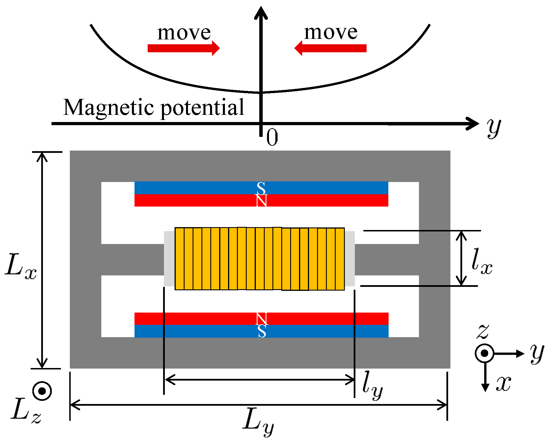
2. Experimental System
3. Problem Statement
4. Model
Derivation of the Model
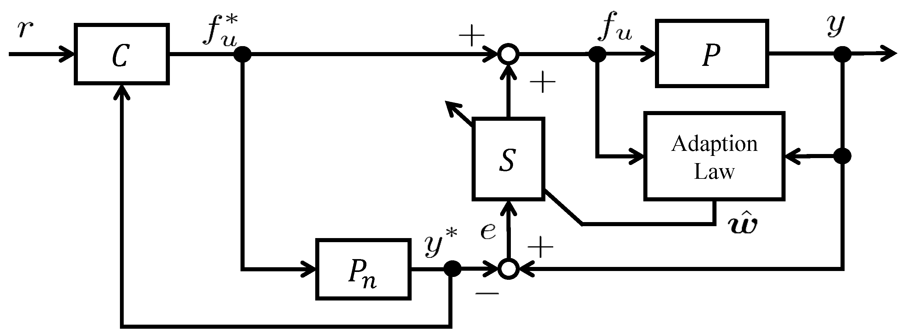
5. Proposed Control Method
5.1. Uncertainty Estimation
5.2. SMC with Uncertainty Compensation
5.3. Shape Parameter Identification of Generalized Gaussian Kernel
5.4. Summary of Proposed Method
- Step 1:
- Observe the stage position y using the sensor.
- Step 2:
- Observe the stage velocity by differentiating y.
- Step 3:
- Update the shape parameters, and , according to the procedure in Section 5.3.
- Step 4:
- Step 5:
- Calculate the ideal operation amount using Equation (32).
- Step 6:
6. Verification
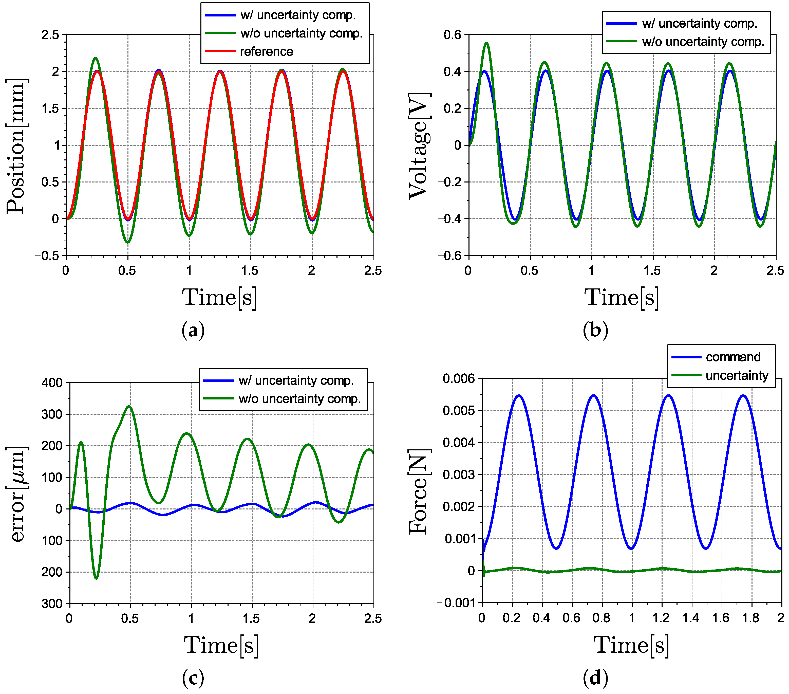
6.1. Simulation
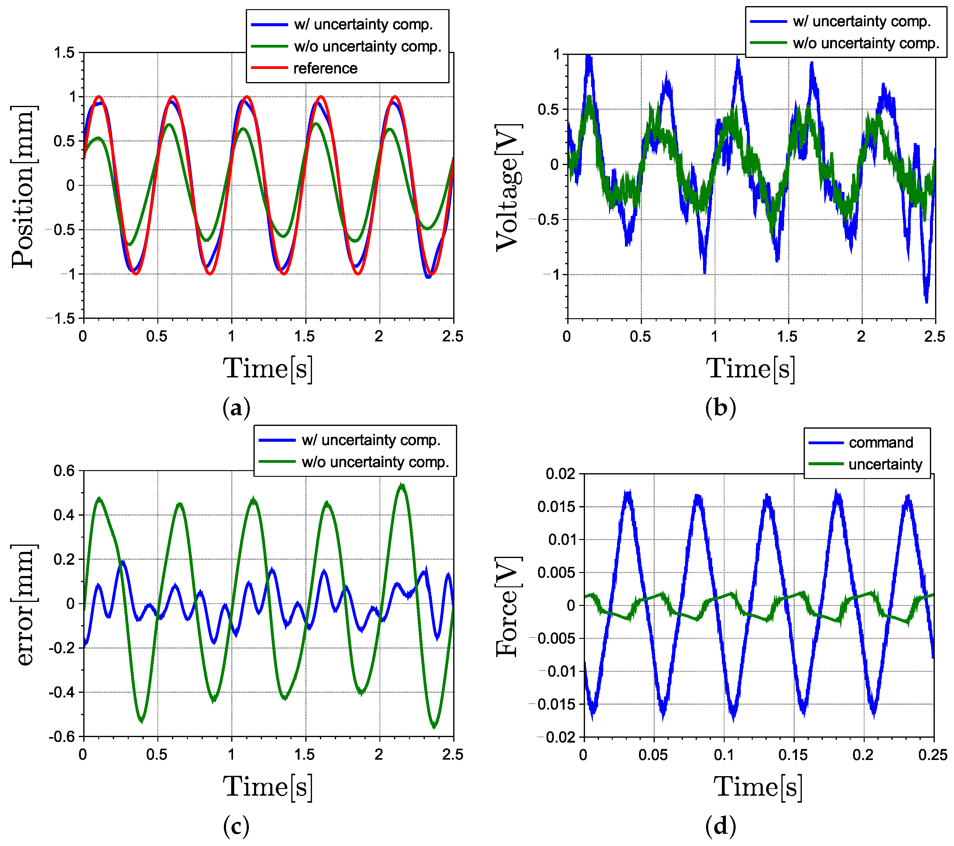
6.2. Experiment
7. Conclusions
Author Contributions
Funding
Data Availability Statement
Conflicts of Interest
References
- Hsiao, H.H.; Wang, K.J. GAGAN: Global Attention Generative Adversarial Networks for Semiconductor Advanced Process Control. IEEE Trans. Semicond. Manuf. 2023, 37, 115–123. [Google Scholar] [CrossRef]
- Kanarik, K.J.; Osowiecki, W.T.; Lu, Y.; Talukder, D.; Roschewsky, N.; Park, S.N.; Kamon, M.; Fried, D.M.; Gottscho, R.A. Human–machine collaboration for improving semiconductor process development. Nature 2023, 616, 707–711. [Google Scholar] [CrossRef]
- Lee, C.Y.; Wu, C.M.; Hsu, C.Y.; Xie, H.H.; Fang, Y.H. Lithography reticle scheduling in semiconductor manufacturing. Eng. Optim. 2023, 1–19. [Google Scholar] [CrossRef]
- Malkin, A.; He, T. The geoeconomics of global semiconductor value chains: Extraterritoriality and the US-China technology rivalry. Rev. Int. Political Econ. 2023, 1–26. [Google Scholar] [CrossRef]
- Hager, A.; Güniat, L.; Morgan, N.; Ramanandan, S.P.; Rudra, A.; Piazza, V.; i Morral, A.F.; Dede, D. The implementation of thermal and UV nanoimprint lithography for selective area epitaxy. Nanotechnology 2023, 34, 445301. [Google Scholar] [CrossRef]
- Fan, S.K.S.; Chen, M.S.; Hsu, C.Y.; Park, Y.J. An artificial intelligence transformation model–pod redesign of photomasks in semiconductor manufacturing. J. Ind. Prod. Eng. 2023, 1–16. [Google Scholar] [CrossRef]
- Sawlani, K.; Mesbah, A. Perspectives on artificial intelligence for plasma-assisted manufacturing in semiconductor industry. In Artificial Intelligence in Manufacturing; Academic Press: Cambridge, MA, USA, 2024; pp. 97–138. [Google Scholar]
- Deng, M.; Iwai, Z.; Mizumoto, I. Robust parallel compensator design for output feedback stabilization of plants with structured uncertainty. Syst. Control Lett. 1999, 36, 193–198. [Google Scholar] [CrossRef]
- Yang, G. Asymptotic tracking with novel integral robust schemes for mismatched uncertain nonlinear systems. Int. J. Robust Nonlinear Control 2023, 33, 1988–2002. [Google Scholar] [CrossRef]
- Badings, T.; Romao, L.; Abate, A.; Parker, D.; Poonawala, H.A.; Stoelinga, M.; Jansen, N. Robust control for dynamical systems with non-gaussian noise via formal abstractions. J. Artif. Intell. Res. 2023, 76, 341–391. [Google Scholar] [CrossRef]
- Gutiérrez-Oribio, D.; Tzortzopoulos, G.; Stefanou, I.; Plestan, F. Earthquake control: An emerging application for robust control. theory and experimental tests. IEEE Trans. Control Syst. Technol. 2023, 31, 1747–1761. [Google Scholar] [CrossRef]
- Perrusquia, A.; Yu, W. Robust control under worst-case uncertainty for unknown nonlinear systems using modified reinforcement learning. Int. J. Robust Nonlinear Control 2020, 30, 2920–2936. [Google Scholar] [CrossRef]
- Husain, S.S.; Kadhim, M.Q.; Al-Obaidi, A.S.M.; Hasan, A.F.; Humaidi, A.J.; Al Husaeni, D.N. Design of robust control for vehicle steer-by-wire system. Indones. J. Sci. Technol. 2023, 8, 197–216. [Google Scholar] [CrossRef]
- Yoshida, R.; Tanigawa, Y.; Okajima, H.; Matsunaga, N. A design method of model error compensator for systems with polytopic-type uncertainty and disturbances. SICE J. Control Meas. Syst. Integr. 2021, 14, 119–127. [Google Scholar] [CrossRef]
- Yang, C.; Xia, Y. Interval uncertainty-oriented optimal control method for spacecraft attitude control. IEEE Trans. Aerosp. Electron. Syst. 2023, 59, 5460–5471. [Google Scholar] [CrossRef]
- Wang, X.; Chen, Z.; Yuan, Z. Output tracking based on extended observer for nonlinear uncertain systems. arXiv 2023, arXiv:2302.05079. [Google Scholar]
- Deng, M.; Inoue, A.; Zhu, Q. An integrated study procedure on real-time estimation of time-varying multi-joint human arm viscoelasticity. Trans. Inst. Meas. Control 2011, 33, 919–941. [Google Scholar] [CrossRef]
- Jaeger, H. Adaptive nonlinear system identification with echo state networks. In NIPS’02: Proceedings of the 15th International Conference on Neural Information Processing Systems; MIT Press: Cambridge, MA, USA, 2002; Volume 15. [Google Scholar]
- Glentis, G.O.; Berberidis, K.; Theodoridis, S. Efficient least squares adaptive algorithms for FIR transversal filtering. IEEE Signal Process. Mag. 1999, 16, 13–41. [Google Scholar] [CrossRef]
- Hollweg, G.V.; Dias de Oliveira Evald, P.J.; Milbradt, D.M.C.; Tambara, R.V.; Gründling, H.A. Lyapunov stability analysis of discrete-time robust adaptive super-twisting sliding mode controller. Int. J. Control 2023, 96, 614–627. [Google Scholar] [CrossRef]
- Abdelrhman, O.M.; Sen, L. Robust adaptive filtering algorithms based on the half-quadratic criterion. Signal Process. 2023, 202, 108775. [Google Scholar] [CrossRef]
- Hoshina, T.; Deng, M. A Nonlinear Control of Linear Slider Considering Position Dependence of Interlinkage Flux. Machines 2022, 10, 522. [Google Scholar] [CrossRef]
- Deng, M.; Inoue, A.; Goto, S. Operator based Thermal Control of an Aluminum Plate with a Peltier Device. Int. J. Innov. Comput. Inf. Control 2008, 4, 3219–3229. [Google Scholar]
- Gao, X.; Yang, Q.; Zhang, J. Multi-objective optimisation for operator-based robust nonlinear control design for wireless power transfer systems. Int. J. Adv. Mechatron. Syst. 2022, 9, 203–210. [Google Scholar] [CrossRef]
- Bu, N.; Wang, X. Swing-up design of double inverted pendulum by using passive control method based on operator theory. Int. J. Adv. Mechatron. Syst. 2023, 10, 1–7. [Google Scholar] [CrossRef]
- Bu, N.; Zhang, Y.; Zhang, Y.; Morohoshi, Y.; Deng, M. Robust Control for Hysteretic Micro-hand Actuator using Robust Right Coprime Factorization. IEEE Trans. Autom. Control 2023, 1–7. [Google Scholar] [CrossRef]
- Wang, Z.; Zhou, R.; Hu, C.; Zhu, Y. Online Iterative Learning Compensation Method Based on Model Prediction for Trajectory Tracking Control Systems. IEEE Trans. Ind. Inform. 2022, 18, 415–425. [Google Scholar] [CrossRef]
- Li, Y.; Luo, P.; Peng, Y.; Liu, Z. Model Free iterative learning for table motion control of lithography machine. In Proceedings of the 2023 8th International Conference on Information Systems Engineering (ICISE), Dalian, China, 23–25 June 2023; pp. 47–50. [Google Scholar]
- Ohnishi, W.; Strijbosch, N.; Oomen, T. State-tracking iterative learning control in frequency domain design for improved intersample behavior. Int. J. Robust Nonlinear Control 2023, 33, 4009–4027. [Google Scholar] [CrossRef]
- Ishii, H.; Manabe, T.; Wakui, S. Reinterpretation of PDD2 compensator embedded in position control for pneumatic stage. J. Adv. Mech. Des. Syst. Manuf. 2019, 13, JAMDSM0074. [Google Scholar] [CrossRef]
- Saito, D.; Wakui, S. Trial of applying the unbalance vibration compensator to axial position of the rotor with AMB. In Proceedings of the 2017 International Conference on Advanced Mechatronic Systems (ICAMechS), Xiamen, China, 6–9 December 2017; pp. 249–254. [Google Scholar]
- Dhavalikar, M.; Dingare, S.; Patle, B. Prediction of Positioning Accuracy and Settling Time of Double Acting Single Rod Pneumatic Cylinder Using SIMULINK. Int. J. COMADEM 2024, 27, 25–29. [Google Scholar]
- Liu, W.; Pokharel, P.P.; Principe, J.C. The kernel least-mean-square algorithm. IEEE Trans. Signal Process. 2008, 56, 543–554. [Google Scholar] [CrossRef]
- Yu, X.; Feng, Y.; Man, Z. Terminal sliding mode control–an overview. IEEE Open J. Ind. Electron. Soc. 2020, 2, 36–52. [Google Scholar] [CrossRef]
- Shtessel, Y.; Edwards, C.; Fridman, L.; Levant, A. Sliding Mode Control and Observation; Springer: New York, NY, USA, 2014; Volume 10. [Google Scholar]
- Levant, A. Sliding order and sliding accuracy in sliding mode control. Int. J. Control 1993, 58, 1247–1263. [Google Scholar] [CrossRef]
- Zhihong, M.; Paplinski, A.P.; Wu, H.R. A robust MIMO terminal sliding mode control scheme for rigid robotic manipulators. IEEE Trans. Autom. Control 1994, 39, 2464–2469. [Google Scholar] [CrossRef]
- Zhao, H.; Xiang, W.; Lv, S. A variable parameter LMS algorithm based on generalized maximum correntropy criterion for graph signal processing. IEEE Trans. Signal Inf. Process. Netw. 2023, 9, 140–151. [Google Scholar] [CrossRef]
- Chen, Z.; Wang, C.; Wang, H.; Ma, Y.; Liang, G.; Wu, X. Heterogeneous Sensor Information Fusion based on Kernel Adaptive Filtering for UAVs’ Localization. In Proceedings of the 2017 IEEE International Conference on Information and Automation (ICIA), Macao, China, 18–20 July 2017; pp. 171–176. [Google Scholar] [CrossRef]
- Xiao, Y.; Yan, W.; Doğançay, K.; Ni, H.; Wang, W. Multikernel adaptive filtering over graphs based on normalized LMS algorithm. Signal Process. 2024, 214, 109230. [Google Scholar] [CrossRef]
- Shi, L.; Lu, R.; Liu, Z.; Yin, J.; Chen, Y.; Wang, J.; Lu, L. An Improved Robust Kernel Adaptive Filtering Method for Time Series Prediction. IEEE Sens. J. 2023, 23, 21463–21473. [Google Scholar] [CrossRef]
- Meng, L.; Hirayama, T.; Oyanagi, S. Underwater-drone with panoramic camera for automatic fish recognition based on deep learning. IEEE Access 2018, 6, 17880–17886. [Google Scholar] [CrossRef]
- Bi, S.; Qu, X.; Ma, L.; Shen, T.; Han, C. Apple grading method based on ordered partition neural network. In Proceedings of the 2021 International Conference on Advanced Mechatronic Systems (ICAMechS), Tokyo, Japan, 9–12 December 2021; pp. 200–205. [Google Scholar]
- Zhao, Y.; Niu, B.; Zong, G.; Zhao, X.; Alharbi, K.H. Neural network-based adaptive optimal containment control for non-affine nonlinear multi-agent systems within an identifier-actor-critic framework. J. Frankl. Inst. 2023, 360, 8118–8143. [Google Scholar] [CrossRef]
- Kurani, A.; Doshi, P.; Vakharia, A.; Shah, M. A comprehensive comparative study of artificial neural network (ANN) and support vector machines (SVM) on stock forecasting. Ann. Data Sci. 2023, 10, 183–208. [Google Scholar] [CrossRef]
- Huang, F.; Xiong, H.; Chen, S.; Lv, Z.; Huang, J.; Chang, Z.; Catani, F. Slope stability prediction based on a long short-term memory neural network: Comparisons with convolutional neural networks, support vector machines and random forest models. Int. J. Coal Sci. Technol. 2023, 10, 18. [Google Scholar] [CrossRef]
- Mahesh, P.V.; Meyyappan, S.; Alla, R. Support Vector Regression Machine Learning based Maximum Power Point Tracking for Solar Photovoltaic systems. Int. J. Electr. Comput. Eng. Syst. 2023, 14, 100–108. [Google Scholar]
- Labbadi, M.; Cherkaoui, M. Robust adaptive nonsingular fast terminal sliding-mode tracking control for an uncertain quadrotor UAV subjected to disturbances. ISA Trans. 2020, 99, 290–304. [Google Scholar] [CrossRef]
- Diana, D.; Carline, M.J. Hybrid metaheuristic method of ABC kernel filtering for nonlinear acoustic echo cancellation. Appl. Acoust. 2023, 210, 109443. [Google Scholar] [CrossRef]
- Novey, M.; Adali, T.; Roy, A. A complex generalized Gaussian distribution—Characterization, generation, and estimation. IEEE Trans. Signal Process. 2009, 58, 1427–1433. [Google Scholar] [CrossRef]
- Deng, M.; Wen, S.; Inoue, A. Sensorless anti-swing robust nonlinear control for travelling crane system using SVR with generalized Gaussian function and robust right coprime factorization. Trans. Soc. Instrum. Control Eng. 2011, 47, 366–373. [Google Scholar] [CrossRef]


| Symbol | Value | Unit | Symbol | Value | Unit |
|---|---|---|---|---|---|
| m | 625,000 | - | |||
| c | 5000 | - | |||
| k | 10 | - | |||
| R | 5,250,000 | - | |||
| L | 5000 | - | |||
| 500 | - | ||||
| 200 | - | ||||
| 100 | - | ||||
| - | |||||
| - | |||||
| 100 | |||||
| - | |||||
| - | |||||
| 10 | - | 10 | - | ||
| 100 | - | 7 | - | ||
| N | 100 | - |
Disclaimer/Publisher’s Note: The statements, opinions and data contained in all publications are solely those of the individual author(s) and contributor(s) and not of MDPI and/or the editor(s). MDPI and/or the editor(s) disclaim responsibility for any injury to people or property resulting from any ideas, methods, instructions or products referred to in the content. |
© 2024 by the authors. Licensee MDPI, Basel, Switzerland. This article is an open access article distributed under the terms and conditions of the Creative Commons Attribution (CC BY) license (https://creativecommons.org/licenses/by/4.0/).
Share and Cite
Hoshina, T.; Yamada, T.; Deng, M. Perfect Tracking Control of Linear Sliders Using Sliding Mode Control with Uncertainty Estimation Mechanism. Machines 2024, 12, 212. https://doi.org/10.3390/machines12040212
Hoshina T, Yamada T, Deng M. Perfect Tracking Control of Linear Sliders Using Sliding Mode Control with Uncertainty Estimation Mechanism. Machines. 2024; 12(4):212. https://doi.org/10.3390/machines12040212
Chicago/Turabian StyleHoshina, Tomoya, Takato Yamada, and Mingcong Deng. 2024. "Perfect Tracking Control of Linear Sliders Using Sliding Mode Control with Uncertainty Estimation Mechanism" Machines 12, no. 4: 212. https://doi.org/10.3390/machines12040212