

A Generalised Intelligent Bearing Fault Diagnosis Model Based on a Two-Stage Approach


Abstract
:1. Introduction
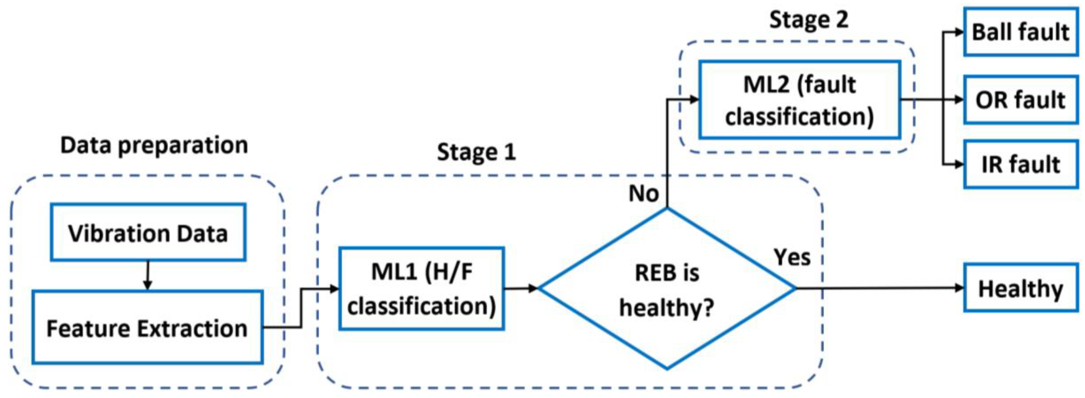
2. Methodology
2.1. Datasets for Training and Testing in Model Development
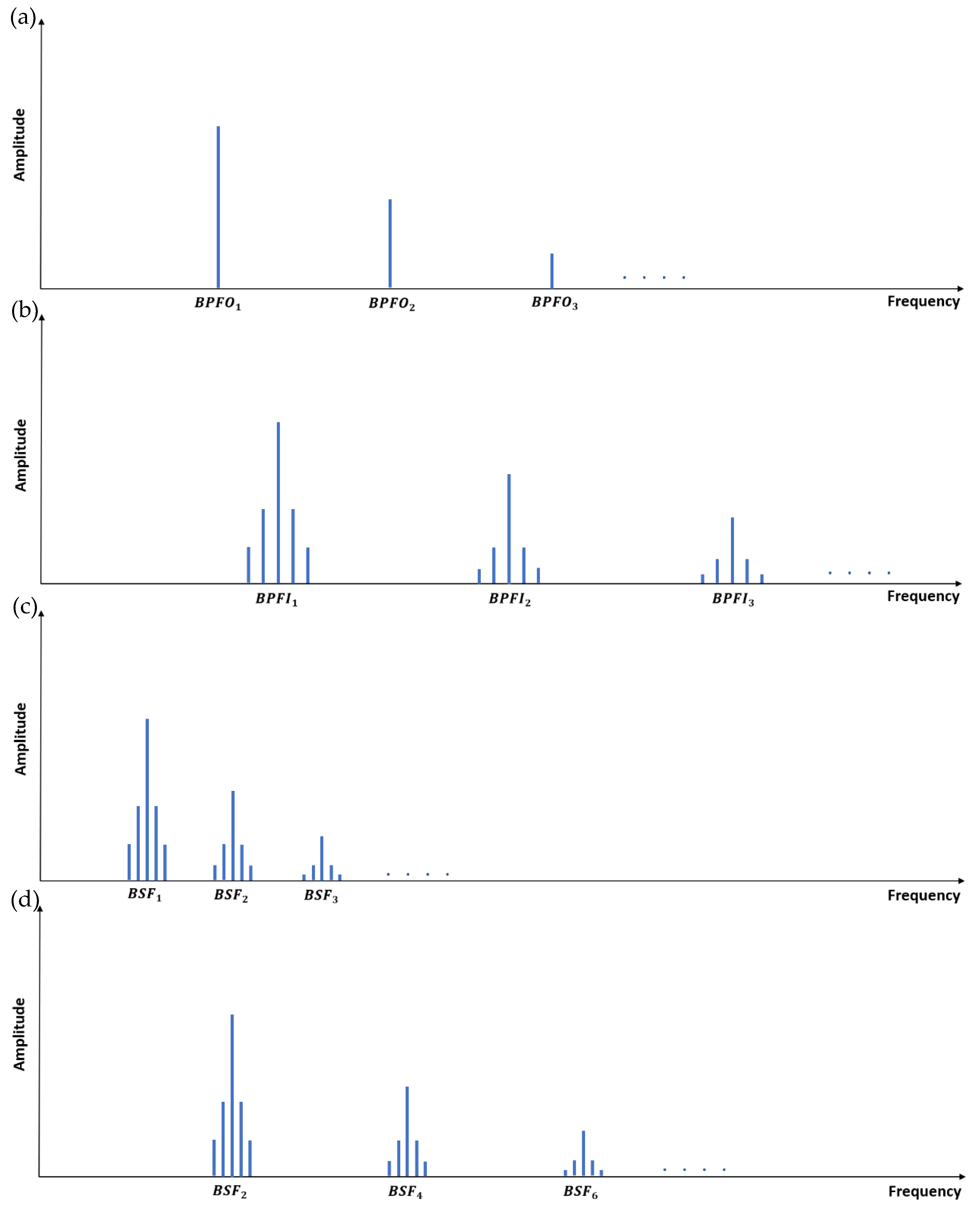
2.2. Feature Extraction Process
- BCFs and their harmonics (9 features):
- ▪
- .
- ▪
- .
- ▪
- .
- Sidebands for BPFIs and BSFs (24 features):
- ▪
- .
- ▪
- .
- ▪
- .
- ▪
- .
- ▪
- .
- ▪
- .
2.3. ML Techniques Used in This Study
2.3.1. SVM
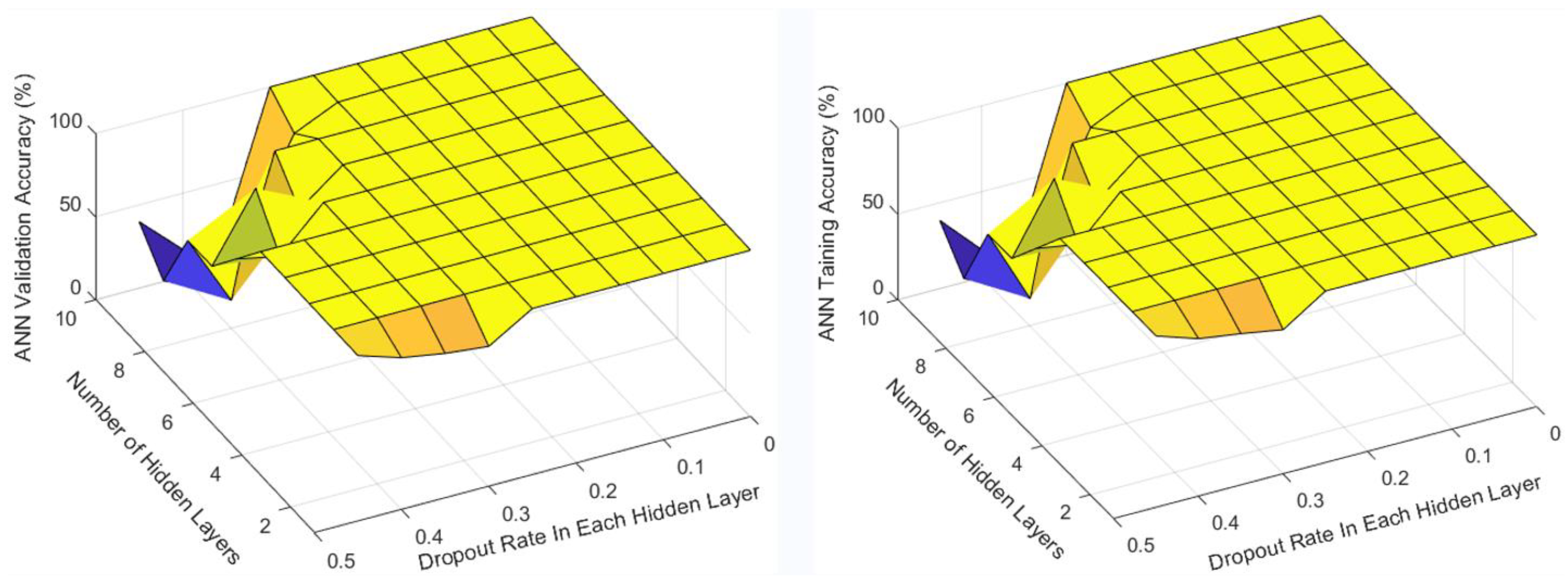
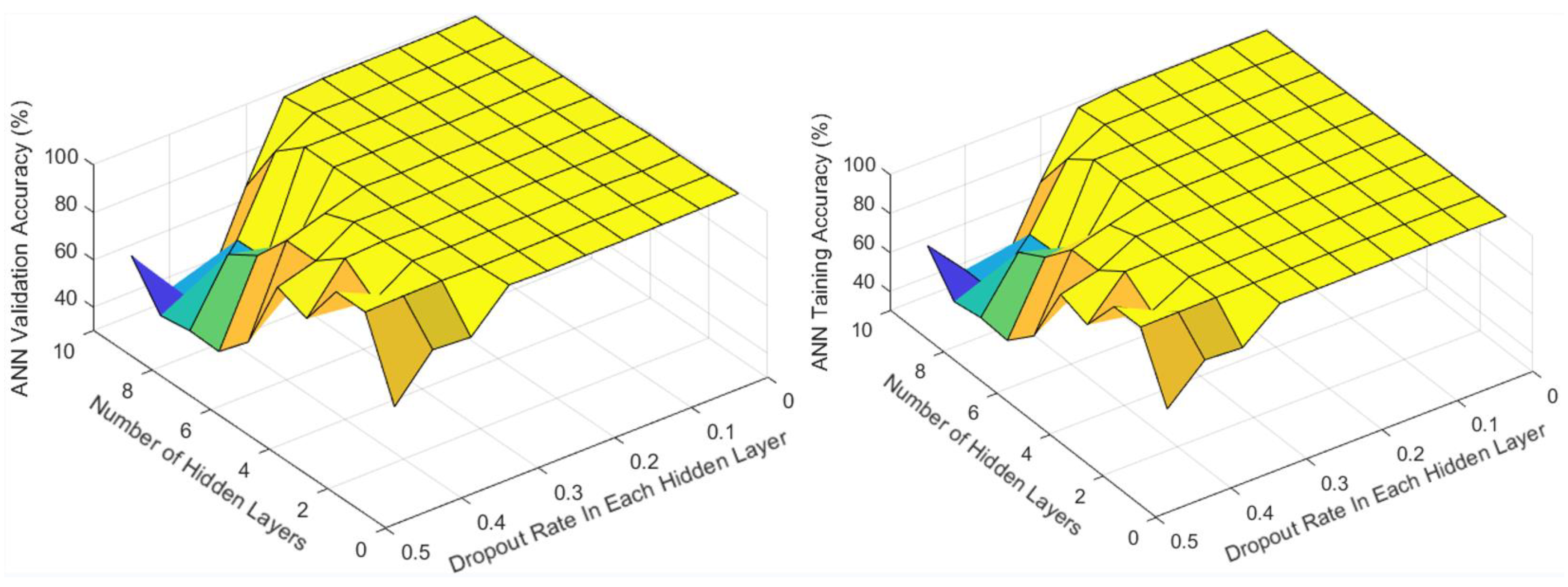
2.3.2. ANN
2.3.3. MLR
3. Results
3.1. Model Training Results
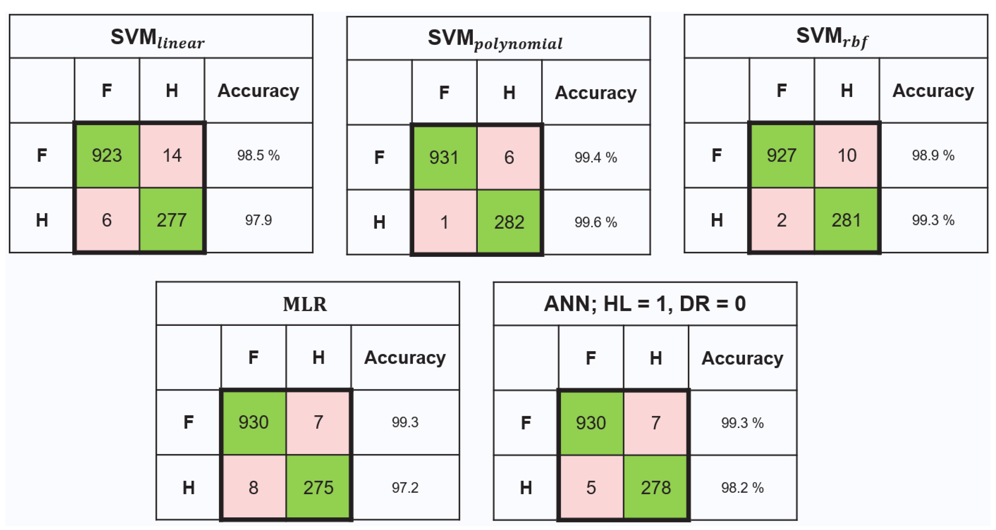
3.1.1. Stage-1 Model (ML1): Classification of Healthy from Faulty Bearings
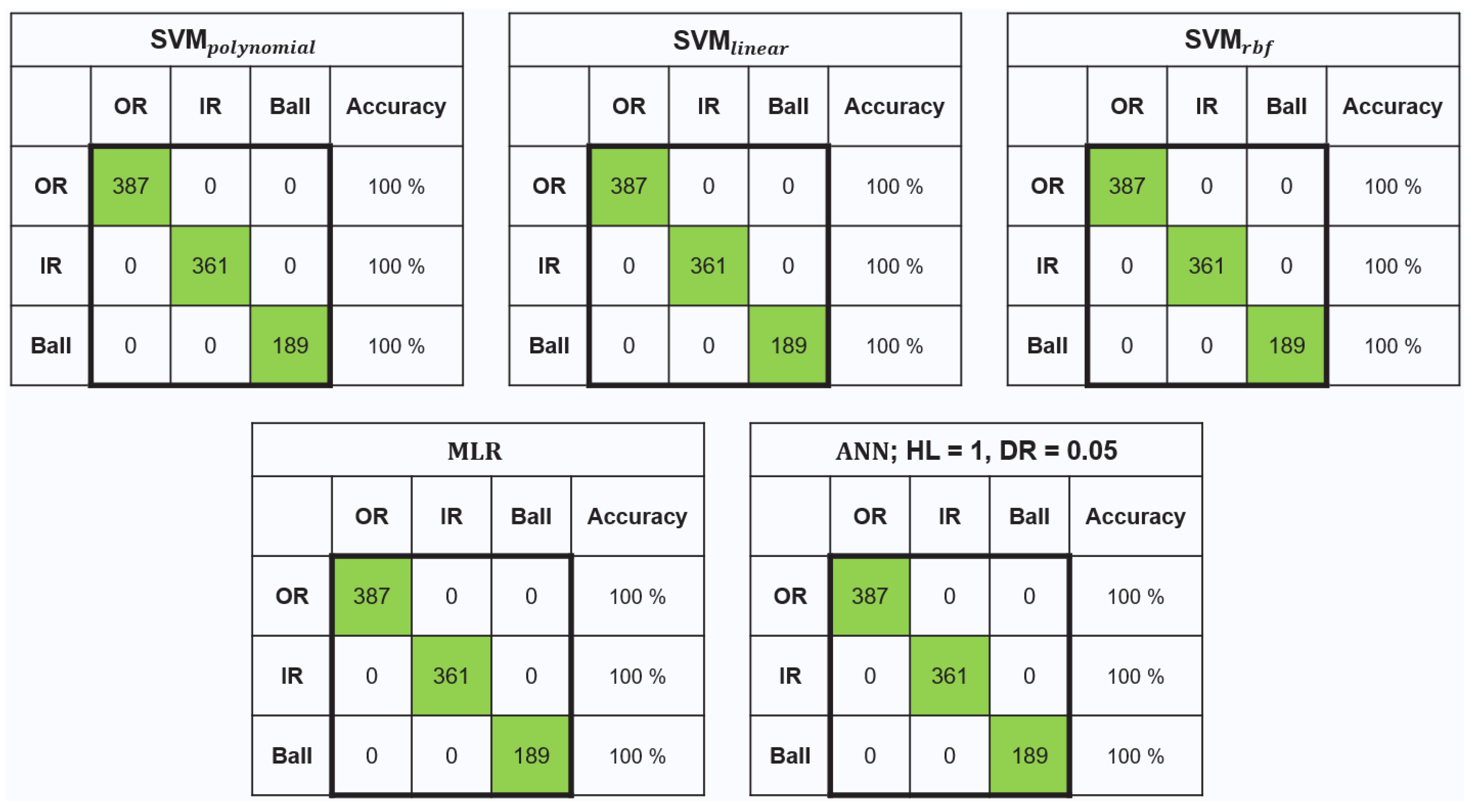
3.1.2. Stage-2 Model (ML2): Classification of Bearing Faults
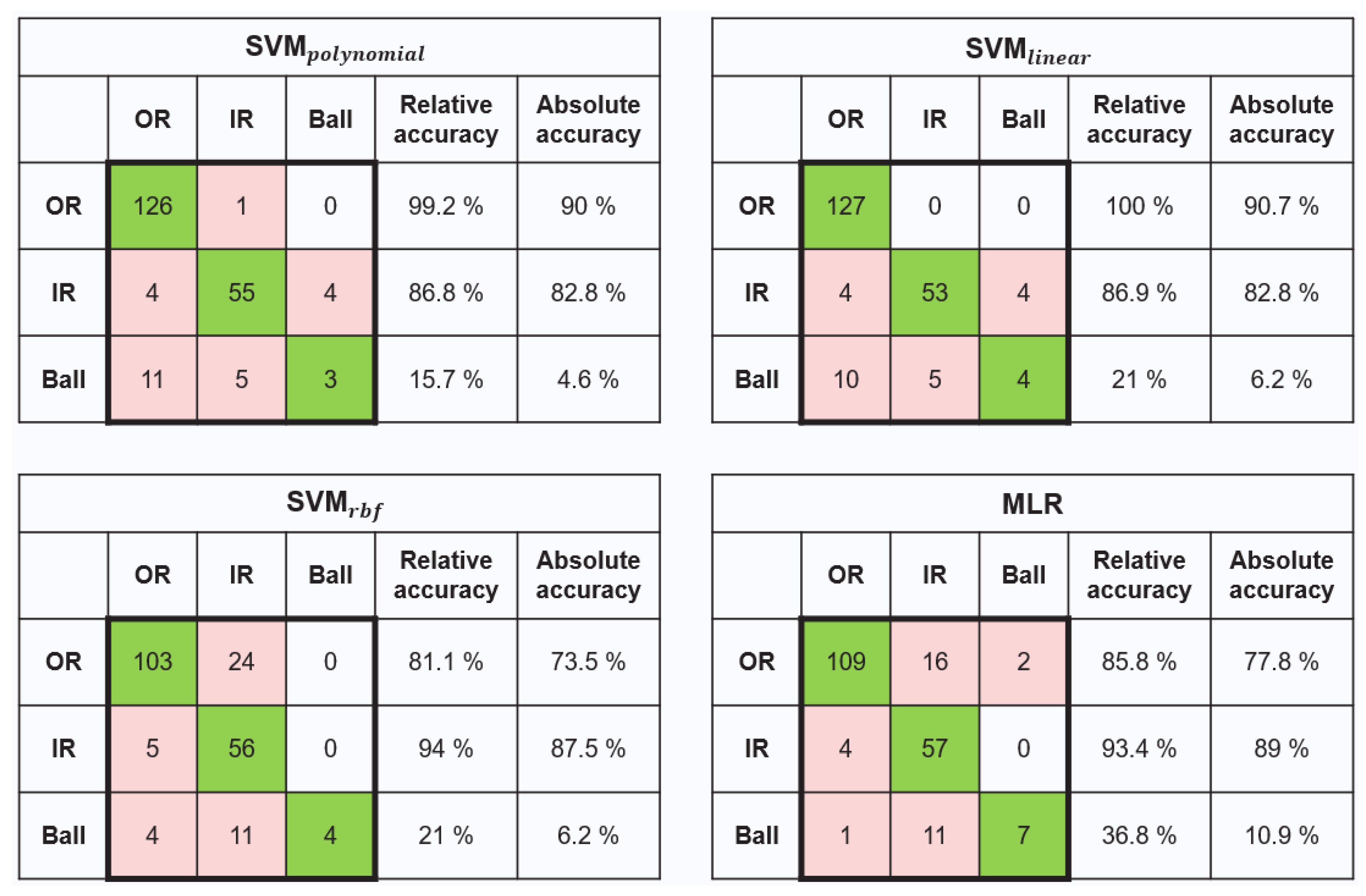
3.2. Model Test Results
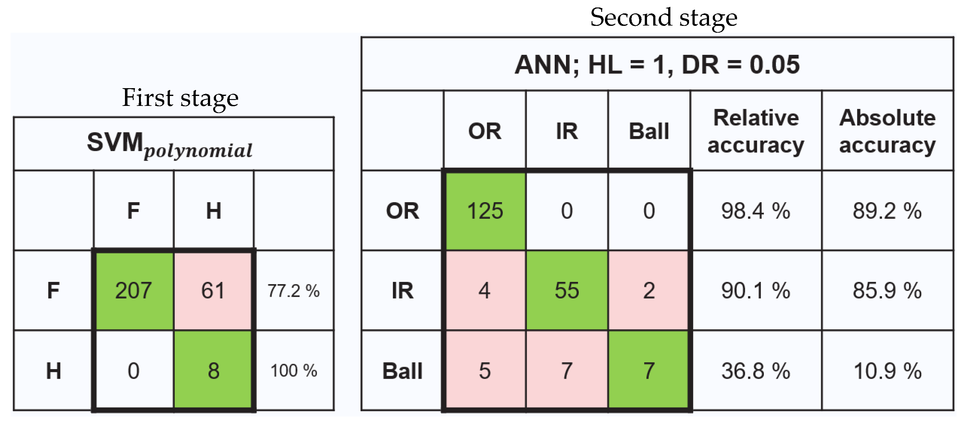
3.2.1. Test the Two-Stage Model with the CWRU Dataset
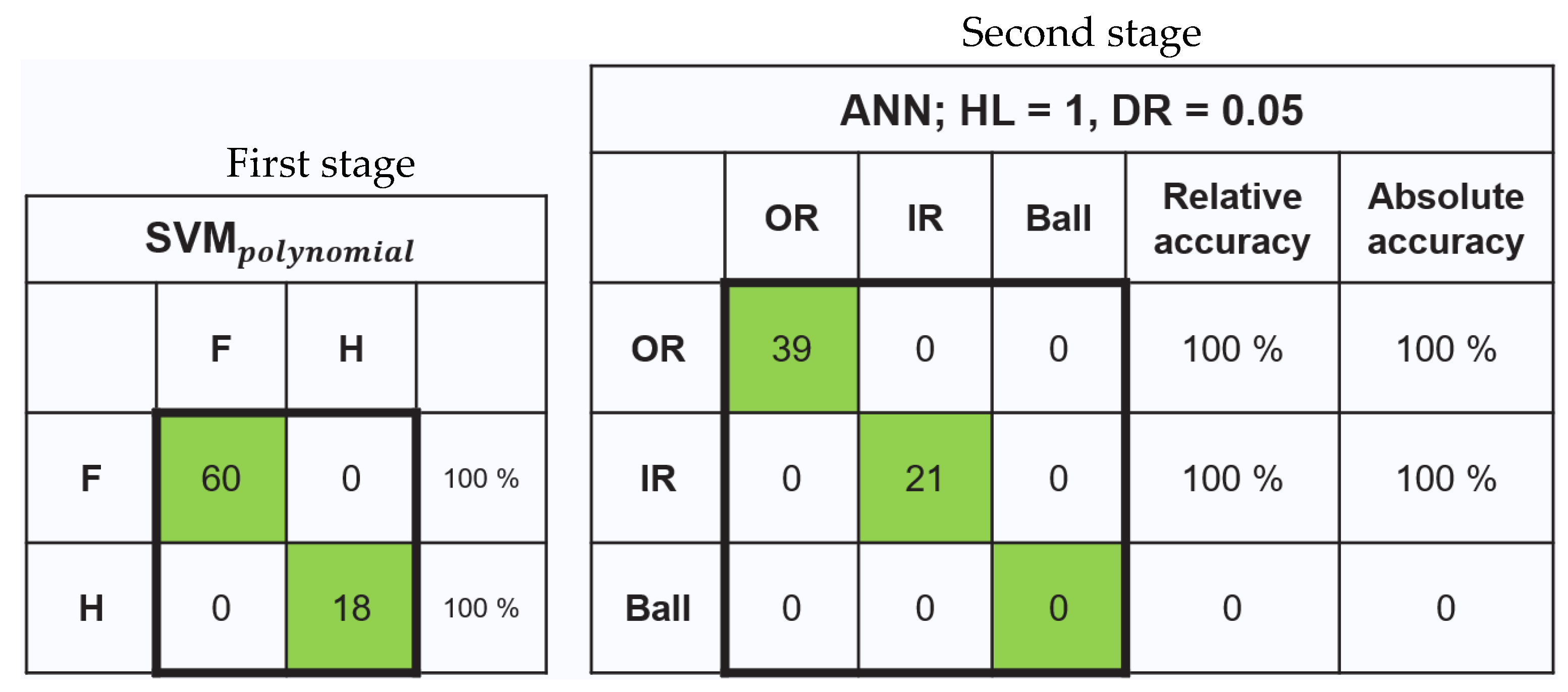
3.2.2. Test the Two-Stage Model with the MFPT Dataset
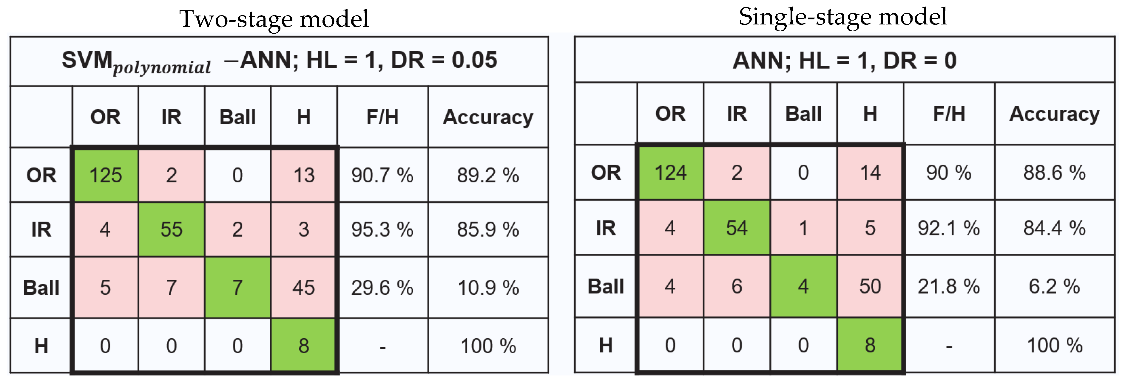
3.3. Compare the Two-Stage Model with a Single-Stage Model
4. Conclusions
Author Contributions
Funding
Data Availability Statement
Conflicts of Interest
Abbreviations
| ANN | Artificial neural network |
| BCF | Bearing characteristic frequency |
| BPFI | Ball pass frequency inner race |
| BPFO | Ball pass frequency outer race |
| BSF | Ball spin frequency |
| CNN | Convolutional neural networks |
| CPW | Cepstrum pre-whitening |
| CWRU | Case Western Reserve University |
| DNN | Deep neural network |
| DR | Dropout rate |
| HFRT | High-frequency resonance technique |
| HL | Hidden layers |
| IR | Inner ring |
| LR | Logistic regression |
| MFPT | Machinery Failure Prevention Technology |
| MLP | Multi-layer perceptron |
| MLR | Multinomial logistic regressions |
| ML | Machine learning |
| OR | Outer ring |
| RBF | Radial basis function |
| REB | Rolling element bearing |
| RNN | Recurrent neural networks |
| SB | Side band |
| SVM | Support vector machine |
Appendix A. I2BS Healthy Bearing Data Synthesis Process
Appendix B. Optimization Results of the ANN for the First Stage of the Fault Diagnosis

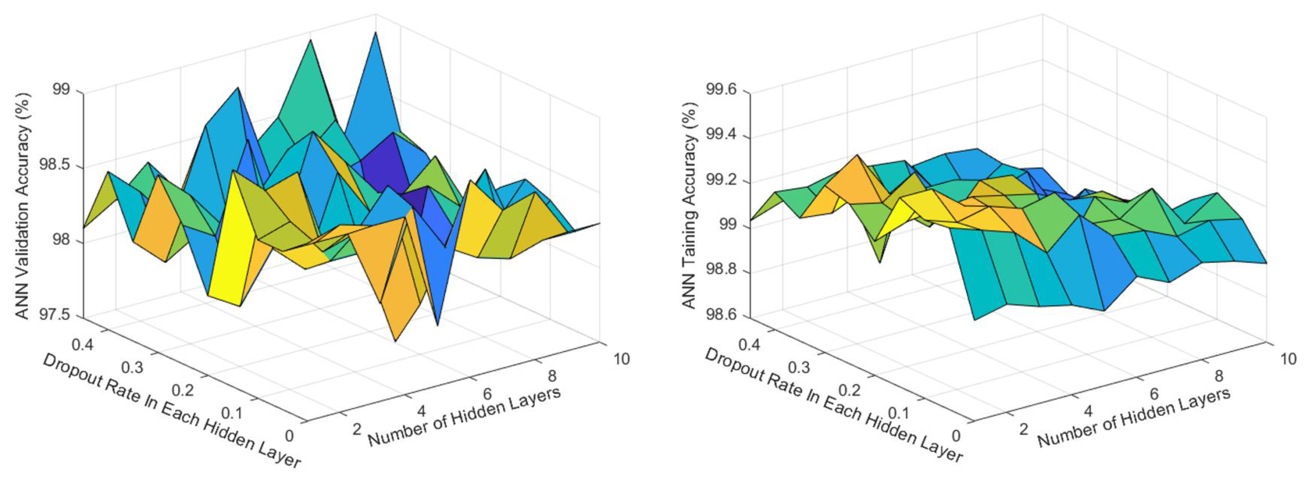
Appendix C. Optimization Results of the ANN for the Second Stage of the Fault Diagnosis

Appendix D. The Test Results of the SVMs and MLR in the Second Stage

Appendix E. Optimization Results of the ANN for the Single-Stage Model

References
- Ambrożkiewicz, B.; Syta, A.; Georgiadis, A.; Gassner, A.; Litak, G.; Meier, N. Intelligent Diagnostics of Radial Internal Clearance in Ball Bearings with Machine Learning Methods. Sensors 2023, 23, 5875. [Google Scholar] [CrossRef] [PubMed]
- Yang, F.; Song, M.; Ma, X.; Guo, N.; Xue, Y. Research on H7006C Angular Contact Ball Bearing Slipping Behavior under Operating Conditions. Lubricants 2023, 11, 298. [Google Scholar] [CrossRef]
- Wu, C.; Yang, K.; Ni, J.; Lu, S.; Yao, L.; Li, X. Investigations for Vibration and Friction Torque Behaviors of Thrust Ball Bearing with Self-Driven Textured Guiding Surface. Friction 2023, 11, 894–910. [Google Scholar] [CrossRef]
- Toma, R.N.; Gao, Y.; Piltan, F.; Im, K.; Shon, D.; Yoon, T.H.; Yoo, D.S.; Kim, J.M. Classification Framework of the Bearing Faults of an Induction Motor Using Wavelet Scattering Transform-Based Features. Sensors 2022, Vol. 22, Page 8958 2022, 22, 8958. [Google Scholar] [CrossRef]
- Guo, C.; Li, L.; Hu, Y.; Yan, J. A Deep Learning Based Fault Diagnosis Method with Hyperparameter Optimization by Using Parallel Computing. IEEE Access 2020, 8, 131248–131256. [Google Scholar] [CrossRef]
- Alshorman, O.; Irfan, M.; Saad, N.; Zhen, D.; Haider, N.; Glowacz, A.; Alshorman, A. A Review of Artificial Intelligence Methods for Condition Monitoring and Fault Diagnosis of Rolling Element Bearings for Induction Motor. Shock Vib. 2020, 2020, 8843759. [Google Scholar] [CrossRef]
- Singh, V.; Gangsar, P.; Porwal, R.; Atulkar, A. Artificial Intelligence Application in Fault Diagnostics of Rotating Industrial Machines: A State-of-the-Art Review. J. Intell. Manuf. 2023, 34, 931–960. [Google Scholar] [CrossRef]
- Li, X.; Zhang, W.; Ding, Q.; Sun, J.Q. Multi-Layer Domain Adaptation Method for Rolling Bearing Fault Diagnosis. Signal Processing 2019, 157, 180–197. [Google Scholar] [CrossRef]
- ALTobi, M.A.S.; Bevan, G.; Wallace, P.; Harrison, D.; Ramachandran, K.P. Fault Diagnosis of a Centrifugal Pump Using MLP-GABP and SVM with CWT. Eng. Sci. Technol. Int. J. 2019, 22, 854–861. [Google Scholar] [CrossRef]
- Hasan, M.J.; Kim, J.M. Bearing Fault Diagnosis under Variable Rotational Speeds Using Stockwell Transform-Based Vibration Imaging and Transfer Learning. Appl. Sci. 2018, 8, 2357. [Google Scholar] [CrossRef]
- Liu, R.; Yang, B.; Zio, E.; Chen, X. Artificial Intelligence for Fault Diagnosis of Rotating Machinery: A Review. Mech. Syst. Signal Process. 2018, 108, 33–47. [Google Scholar] [CrossRef]
- Zhang, S.; Zhang, S.; Wang, B.; Habetler, T.G. Deep Learning Algorithms for Bearing Fault Diagnosticsx—A Comprehensive Review. IEEE Access 2020, 8, 29857–29881. [Google Scholar] [CrossRef]
- Guo, L.; Lei, Y.; Xing, S.; Yan, T.; Li, N. Deep Convolutional Transfer Learning Network: A New Method for Intelligent Fault Diagnosis of Machines with Unlabeled Data. IEEE Trans. Ind. Electron. 2019, 66, 7316–7325. [Google Scholar] [CrossRef]
- Yang, B.; Lei, Y.; Jia, F.; Xing, S. An Intelligent Fault Diagnosis Approach Based on Transfer Learning from Laboratory Bearings to Locomotive Bearings. Mech. Syst. Signal Process. 2019, 122, 692–706. [Google Scholar] [CrossRef]
- Zhang, Y.; Li, S.; Zhang, A.; Li, C.; Qiu, L. A Novel Bearing Fault Diagnosis Method Based on Few-Shot Transfer Learning across Different Datasets. Entropy 2022, 24, 1295. [Google Scholar] [CrossRef]
- Mao, W.; Ding, L.; Tian, S.; Liang, X. Online Detection for Bearing Incipient Fault Based on Deep Transfer Learning. Meas. J. Int. Meas. Confed. 2020, 152, 107278. [Google Scholar] [CrossRef]
- Singh, J.; Azamfar, M.; Li, F.; Lee, J. A Systematic Review of Machine Learning Algorithms for Prognostics and Health Management of Rolling Element Bearings: Fundamentals, Concepts and Applications. Meas. Sci. Technol. 2021, 32, 012001. [Google Scholar] [CrossRef]
- Luo, Y.; Guo, Y. Envelope Analysis Scheme for Multi-Faults Vibration of Gearbox Based on Self-Adaptive Noise Cancellation. In Proceedings of the 2018 Prognostics and System Health Management Conference, Chongqing, China, 26–28 October 2018; pp. 1188–1193. [Google Scholar] [CrossRef]
- Li, H.; Liu, T.; Wu, X.; Chen, Q. Application of EEMD and Improved Frequency Band Entropy in Bearing Fault Feature Extraction. ISA Trans. 2019, 88, 170–185. [Google Scholar] [CrossRef]
- Kiakojouri, A.; Lu, Z.; Mirring, P.; Powrie, H.; Wang, L. A Novel Hybrid Technique Combining Improved Cepstrum Pre-Whitening and High-Pass Filtering for Effective Bearing Fault Diagnosis Using Vibration Data. Sensors 2023, 23, 9048. [Google Scholar] [CrossRef]
- Mathur, A.; Kumar, P.; Harsha, S.P. Ranked Feature-Based Data-Driven Bearing Fault Diagnosis Using Support Vector Machine and Artificial Neural Network. Proc. Inst. Mech. Eng. Part I J. Syst. Control Eng. 2023, 237, 1602–1619. [Google Scholar] [CrossRef]
- Yan, M.; Wang, X.; Wang, B.; Chang, M.; Muhammad, I. Bearing Remaining Useful Life Prediction Using Support Vector Machine and Hybrid Degradation Tracking Model. ISA Trans. 2020, 98, 471–482. [Google Scholar] [CrossRef] [PubMed]
- Kiakojouri, A.; Lu, Z.; Mirring, P.; Powrie, H.; Wang, L. A Generalised Machine Learning Model Based on Multinomial Logistic Regression and Frequency Features for Rolling Bearing Fault Classification. Insight—Non-Destr. Test. Cond. Monit. 2022, 64, 447–452. [Google Scholar] [CrossRef]
- Abdelrhman, A.M.; Ying, L.; Ali, Y.H.; Ahmad, I.; Georgantopoulou, C.G.; Nor, F.M.; Kurniawan, D. Diagnosis Model for Bearing Faults in Rotating Machinery by Using Vibration Signals and Binary Logistic Regression. AIP Conf. Proc. 2020, 2262, 030014. [Google Scholar]
- Parmar, U.; Pandya, D.H. Comparison of the Supervised Machine Learning Techniques Using WPT for the Fault Diagnosis of Cylindrical Roller Bearing. Int. J. Eng. Sci. Technol. 2021, 13, 50–56. [Google Scholar] [CrossRef]
- Bashir, I.; Zaghari, B.; Harvey, T.J.; Weddell, A.S.; White, N.M.; Wang, L. Design and Testing of a Sensing System for Aero-Engine Smart Bearings. Proceedings 2019, 2, 1005. [Google Scholar] [CrossRef]
- Case Western Reserve University Bearing Data Center. 2009. Available online: https://engineering.case.edu/bearingdatacenter (accessed on 6 January 2022).
- Fault Data Sets—Society For Machinery Failure Prevention Technology. Available online: https://www.mfpt.org/fault-data-sets/ (accessed on 12 April 2022).
- Randall, R.B.; Antoni, J. Rolling Element Bearing Diagnostics—A Tutorial. Mech. Syst. Signal Process. 2011, 25, 485–520. [Google Scholar] [CrossRef]
- Gao, X.; Wei, H.; Li, T.; Yang, G. A Rolling Bearing Fault Diagnosis Method Based on LSSVM. Adv. Mech. Eng. 2020, 12, 1–10. [Google Scholar] [CrossRef]
- Hamadache, M.; Jung, J.H.; Park, J.; Youn, B.D. A Comprehensive Review of Artificial Intelligence-Based Approaches for Rolling Element Bearing PHM: Shallow and Deep Learning. JMST Adv. 2019, 1, 125–151. [Google Scholar] [CrossRef]
- Ahmed, H.O.A.; Nandi, A.K.; Delpha, C.; Ahmed, H.O.A.; Nandi, A.K. Intrinsic Dimension Estimation-Based Feature Selection and Multinomial Logistic Regression for Classification of Bearing Faults Using Compressively Sampled Vibration Signals. Entropy 2022, 24, 511. [Google Scholar] [CrossRef]
- Gao, S.; Yu, Y.; Zhang, Y. Reliability Assessment and Prediction of Rolling Bearings Based on Hybrid Noise Reduction and BOA-MKRVM. Eng. Appl. Artif. Intell. 2022, 116, 105391. [Google Scholar] [CrossRef]
- Neupane, D.; Seok, J. Bearing Fault Detection and Diagnosis Using Case Western Reserve University Dataset with Deep Learning Approaches: A Review. IEEE Access 2020, 8, 93155–93178. [Google Scholar] [CrossRef]
- Smith, W.A.; Randall, R.B. Rolling Element Bearing Diagnostics Using the Case Western Reserve University Data: A Benchmark Study. Mech. Syst. Signal Process. 2015, 64–65, 100–131. [Google Scholar] [CrossRef]


| Dataset Name | Bearing Size, mm | Defect Size, mm | Speed, rpm | Load, kN | |||
|---|---|---|---|---|---|---|---|
| PD | Ball | Z | |||||
| I2BS sub-scale | 75 | 9.5 | 20 | 0.4 | 5000, 10,000, 14,000 | 1, 2.5, 9 | 100 |
| CWRU | 38.5 | 7.9 | 9 | 0.177, 0.355, 0.533 | 1720–1797 | N/A | 12, 48 |
| MFPT | 31.6 | 5.97 | 8 | N/A | 1500 | 0.22, 0.44, 0.66, 0.88, 1.11, 1.33 | 48,828, 96,656 |
| Health State | OR Fault | IR Fault | Ball Fault | Healthy | |
|---|---|---|---|---|---|
| Data Source | |||||
| I2BS subscale | 387 | 361 | 189 | 283 * | |
| CWRU | 140 | 64 | 64 | 8 | |
| MFPT | 39 | 21 | 0 | 18 | |
| Health State | Diagnosable (%) | Partial Diagnoseable (%) | Not Diagnosable (%) |
|---|---|---|---|
| OR fault | 78.5 | 12.2 | 9.3 |
| IR fault | 73.4 | 14.1 | 12.5 |
| Ball fault | 10.9 | 10.9 | 78.2 |
Disclaimer/Publisher’s Note: The statements, opinions and data contained in all publications are solely those of the individual author(s) and contributor(s) and not of MDPI and/or the editor(s). MDPI and/or the editor(s) disclaim responsibility for any injury to people or property resulting from any ideas, methods, instructions or products referred to in the content. |
© 2024 by the authors. Licensee MDPI, Basel, Switzerland. This article is an open access article distributed under the terms and conditions of the Creative Commons Attribution (CC BY) license (https://creativecommons.org/licenses/by/4.0/).
Share and Cite
Kiakojouri, A.; Lu, Z.; Mirring, P.; Powrie, H.; Wang, L. A Generalised Intelligent Bearing Fault Diagnosis Model Based on a Two-Stage Approach. Machines 2024, 12, 77. https://doi.org/10.3390/machines12010077
Kiakojouri A, Lu Z, Mirring P, Powrie H, Wang L. A Generalised Intelligent Bearing Fault Diagnosis Model Based on a Two-Stage Approach. Machines. 2024; 12(1):77. https://doi.org/10.3390/machines12010077
Chicago/Turabian StyleKiakojouri, Amirmasoud, Zudi Lu, Patrick Mirring, Honor Powrie, and Ling Wang. 2024. "A Generalised Intelligent Bearing Fault Diagnosis Model Based on a Two-Stage Approach" Machines 12, no. 1: 77. https://doi.org/10.3390/machines12010077