Article

A Three-State Space Modeling Method for Aircraft System Reliability Design

1
School of Mechanical and Precision Instrument Engineering, Xi’an University of Technology, Xi’an 710048, China
2
Xi’an Institute of Optics and Precision Mechanics of CAS, Xi’an 710119, China
3
School of Aeronautics, Northwestern Polytechnical University, Xi’an 710072, China
*
Author to whom correspondence should be addressed.
Machines 2024, 12(1), 13; https://doi.org/10.3390/machines12010013
Submission received: 1 November 2023 / Revised: 7 December 2023 / Accepted: 11 December 2023 / Published: 25 December 2023
(This article belongs to the Special Issue Optimal Design of Aircraft)

Abstract

:
Reliability is an inherent attribute of a system through optimal system design. However, during the aircraft system development process, the reliability evaluation and system function design efforts are often disconnected, leading to a divide between reliability experts and system designers in their work schedule. This disconnect results in an inefficient aircraft system reliability optimization process, known as the “two-skin” phenomenon. To address this issue, a three-state space model is proposed. Firstly, an analysis was conducted on the relationship between the system function architecture developed by the system designers and the reliability evaluation performed by the reliability experts. Secondly, based on the principle of function flow, the state of failure was categorized into “physical failure” and “non-physical failure”. Additionally, a new state of “function loss” was introduced as the third state for the system, in addition to the traditional states of “normal” and “faulty”. Thirdly, through the state of “Function loss”, an effective integration of system fault modes and function modes was achieved, leading to an optimized system reliability model. A three-state space modeling method was then developed by transforming the system function architecture into a system reliability model. Finally, this new model was applied to an aircraft’s rudder and fly-by-wire control system. The results demonstrate that the function architecture at the design stage of the system can be accurately transformed into the new three-state space model. The structure aligns closely with the function architecture and can be effectively utilized in quantitative system reliability calculations. In this way, the process of ensuring system reliability can be seamlessly integrated into the system optimization design process. This integration alleviates the issue of disjointed work between reliability experts and system designers, leading to a more streamlined and efficient aircraft system optimization process.

1. Introduction

An aircraft is composed of three main parts: the airframe, engine, and airborne equipment. Airborne equipment generally refers to independent functional devices installed on the aircraft to complete various flight tasks and ensure flight safety and comfort. It includes dozens of systems, such as the power supply system, flight control system, environmental control system, etc. As the “blood” and “muscle” of the aircraft, airborne equipment is a crucial indicator of the aircraft’s advanced level. In modern advanced aircraft, the value of airborne equipment and systems accounts for 30% to 40% of the total aircraft value. For simplicity, in this paper, the term “aircraft system” refers to airborne equipment [1].
With the development of aircraft system integration, systematization, and full electrification, system design has become increasingly complex, and the reliability issue of aircraft has become increasingly prominent. The fundamental characteristic of system reliability is that a single defect during the design optimization process can affect the entire system, and hidden design defects can lead to future issues in application. Conversely, simultaneous reliability evaluation during the system optimization design process can provide significant economic benefits for subsequent system use. For instance, Boeing Company applied reliability achievements to the design of the Boeing 737 series aircraft, reducing the service and maintenance cost of the series aircraft by 15% [2].
In conclusion, it is essential to conduct reliability evaluation simultaneously during the system optimization design stage [3]. This approach enables the identification of system vulnerabilities in advance, facilitates the improvement of design defects, and ultimately reduces the accident rate during the design stage. Therefore, reliability evaluation during the system design process is of great engineering significance, as it can accelerate the system optimization process, expedite system development, and ultimately reduce life cycle costs.
The reliability evaluation work of the system during the aircraft system optimization design process depends on a reasonable and effective reliability model [4,5,6]. Only by establishing a correct and effective system reliability model can the system reliability be predicted and distributed, and the in-depth analysis of the effects and hazards of failure modes be carried out. Building a system reliability model is essential in reliability design [7,8]. Currently, fault tree analysis (FTA) [9,10], reliability block diagram (RBD) [11,12], failure mode and effect analysis (FMEA) [13,14], event tree (ET) [15], the minimum cut set method [16,17], dynamic fault tree (DFT) [18,19], and Markov chain (MC) [20,21] have mature theoretical foundations. These are the primary technical means of aircraft system reliability evaluation both domestically and internationally.
Typically, reliability experts analyze each system component’s failure modes and effects using FMEA. Subsequently, reliability models such as RBD, ET, FT, and minimum cut set are constructed based on expert knowledge for quantitative reliability calculations. For instance, in Refs. [17,22], the architecture of the aircraft power system is abstracted as a network. System reliability is then evaluated by determining the minimum cut set of the network. Additionally, to address the limitations of FT, RBD, and other models in terms of computational capabilities and fault propagation visualization, methods for transforming these models into equivalent Bayesian networks, Petri nets, and other models have also been studied. For instance, in Ref. [23], a discrete Bayesian network based on a dynamic fault tree was proposed for the reliability evaluation of an integrated modular avionics core processing system. Given that the use of conventional FT and RBD is challenging in terms of handling fault dependencies in aircraft electrical power systems, Ref. [24] developed a Bayesian network modeling method based on the power supply path set and verified the model’s accuracy through several case studies. Given the strong visibility and good dynamic expression capabilities of Petri nets in system modeling, Ref. [25] proposed a reliability modeling method for complex aircraft systems based on Petri nets. Additionally, a Monte Carlo simulation method was developed to solve the model, and the feasibility and accuracy of the method were verified through an example involving the fly-by-wire control system of an aircraft.
However, most of these reliability modeling methods over-rely on the subjective experience of experts, especially for large complex systems, which have complex coupled causality. Even if the same reliability modeling method is used to model one system, the models established by different modelers are likely to be different, making it difficult for experts to judge the rationality of the models [26,27]. System reliability design is a process of iterating the design scheme until the reliability meets the design requirements [8,28]. This means that after the system design specialist completes the function design and forms the function architecture, the reliability specialist still needs to spend considerable time and economic cost on building the reliability model if a modeling approach that relies too heavily on experience is adopted. This eventually leads to the “two-skin” phenomenon where the work between the two specialties of system design and reliability is prone to disconnection, prevarication, and inability to effectively integrate, severely affecting the iterative progress of aircraft system design.
In the absence of, or with reduced reliance on, expert experience, transforming the function architecture during the system design stage into the system reliability model effectively addresses the “two-skin” phenomenon [29]. One method for accomplishing this transformation is through the use of the model-based safety analysis (MBSA) technique. MBSA utilizes system models, such as functional block diagrams or architectural models, and automatically generates fault trees or reliability block diagrams based on the system architecture. These models can then be further analyzed to estimate reliability metrics and assess system safety. It is important to note, however, that while the automated approach can facilitate the transformation from system function architecture to reliability models, it often requires well-defined system models and may still require some manual intervention or expertise to ensure the accuracy and validity of the resulting reliability model. Therefore, it is necessary to explore alternative methods for transforming system function architecture into a reliability model. Additionally, the NASA research report [30] pointed out that since the system design specialist focuses more on system functions while the reliability specialist focuses more on system faults, the key to transforming system function architecture during the system design stage into a system reliability model lies in effectively transforming the function architecture from the function space to the fault space.
In summary, to address the “two-skin” phenomenon between system design and reliability experts and to accelerate the optimization process of aircraft system design, this paper introduces a new state of “function loss” as the third type of state in a system, alongside the two basic states of “normal” and “fault”. We explore a three-state space modeling method that can automatically transform the system function architecture into the system reliability model without relying on expert experience. This research provides a theoretical foundation for effectively integrating system design and reliability evaluation work, ultimately accelerating the optimization process of aircraft system design.
Other chapters of this paper are arranged as follows: Section 2 discusses the basic theory of system design and reliability evaluation and the relationship between them; Section 3 discusses the principle and implementation steps of the newly proposed three-state space modeling method. Section 4 includes case analysis and verification; Section 5 includes conclusions and prospects.

2. Theoretical Basis of Aircraft System Reliability Analysis

This chapter analyzes the reasons for the ineffective integration of system function design and reliability evaluation by examining the aircraft system reliability process during the system optimization design process. The primary reason is that the workspaces of the reliability specialist and system design specialist are distinct, and existing methods cannot directly transform the system function architecture into a system reliability model. Furthermore, as the core task of reliability evaluation lies in reliability modeling, this chapter also summarizes the theoretical foundation of aircraft system reliability modeling.

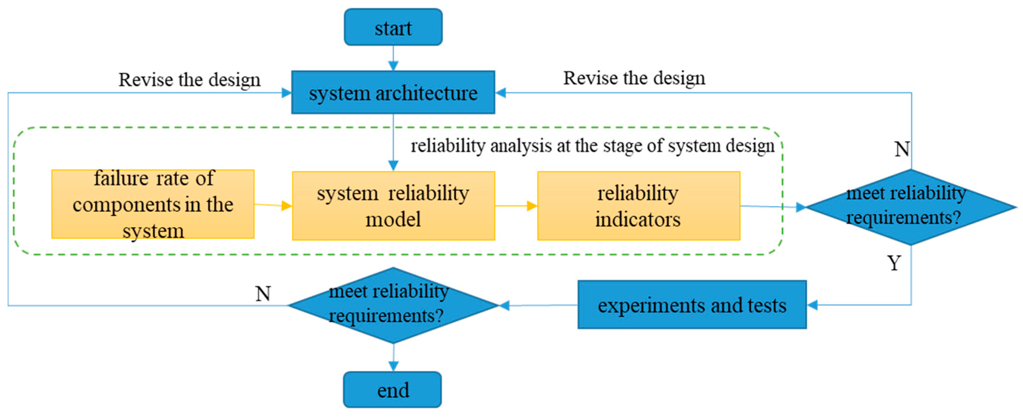
2.1. System Reliability Optimization Process

The system combines interrelated components, forming an organic whole capable of performing specific functions. The system design specialist’s focus is on organically combining components to achieve specific functions from the perspective of function flow. Among them, the system function architecture can describe the function flow between the system and its components. System reliability is the probability that the system completes the specified function in the specified time, and it is an inherent attribute assigned to the system during the design stage.
However, designing a system that meets reliability requirements is an iterative optimization process that requires the cooperation of the system design specialist and reliability specialist [31,32], see Figure 1. Specifically, after the system design specialist completes the functional design, the reliability specialist needs to build a system reliability model based on the system function architecture and perform a reliability evaluation. If the design does not meet reliability index requirements, the system design specialist must optimize the design architecture based on the weak links identified by the reliability specialist. Once the design is optimized, the reliability specialist constructs a new reliability model of the optimized system and evaluates its reliability again until the optimized system design meets reliability requirements.
The effective collaboration and integration of the work between the system design specialist and reliability specialist are crucial in promoting the efficiency of high-reliability system development. However, the system design specialist works in the function space, which describes the function flow: how components are organically combined to complete the given function of the system. Conversely, the reliability specialist works in the fault space, which depicts the fault propagation path: how component-level faults spread and lead to the failure of the system-level function.
In summary, aircraft system design is an optimization process. Aircraft system reliability design involves iterative modeling and calculation during the system design process. As system design and reliability specialists operate in separate spaces, there is a significant gap between the two specialties. Therefore, the key to accelerating the system design optimization process is to bridge this gap. The key to bridging the gap lies in transforming the function space’s system function architecture into the fault space’s system reliability model without relying heavily on expert experience.

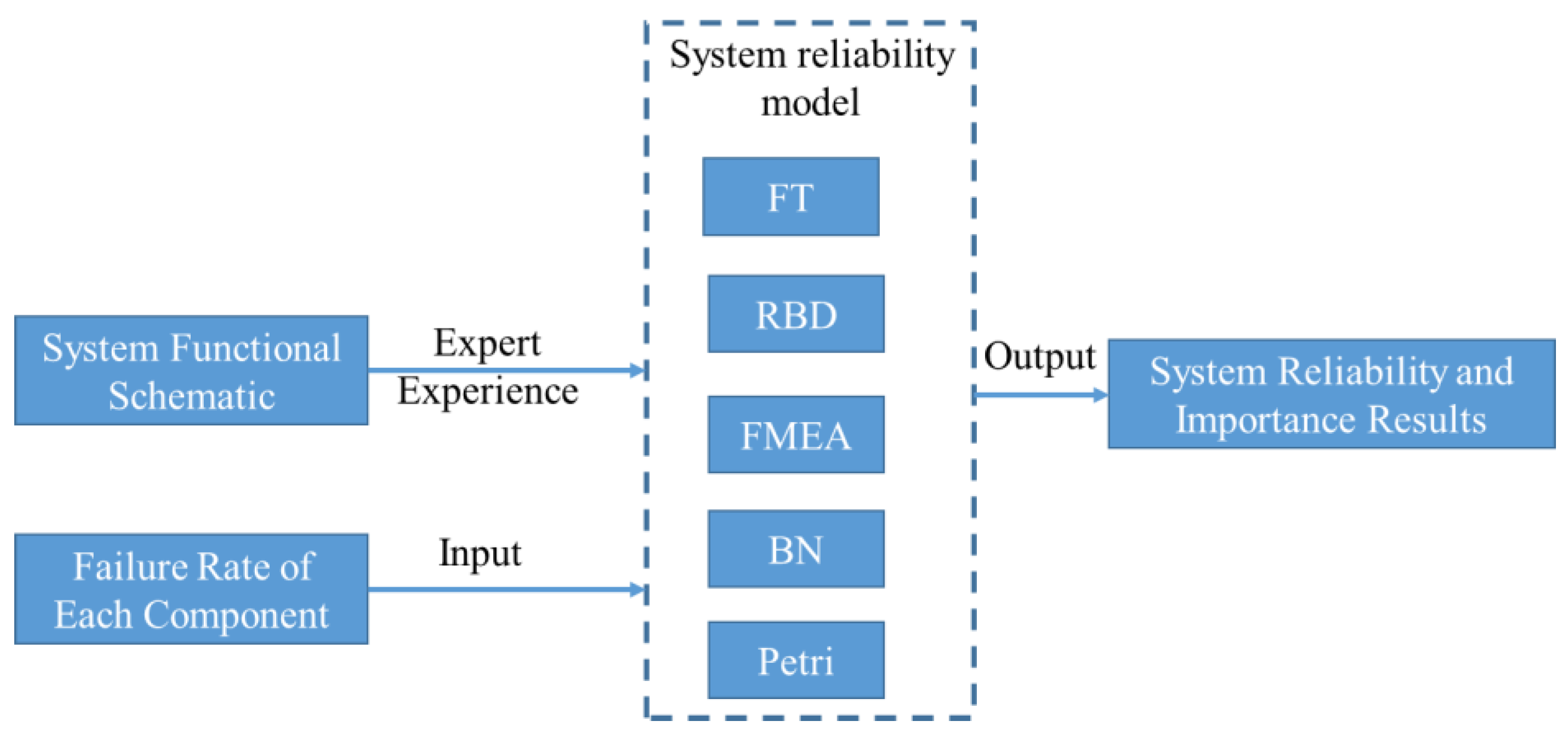
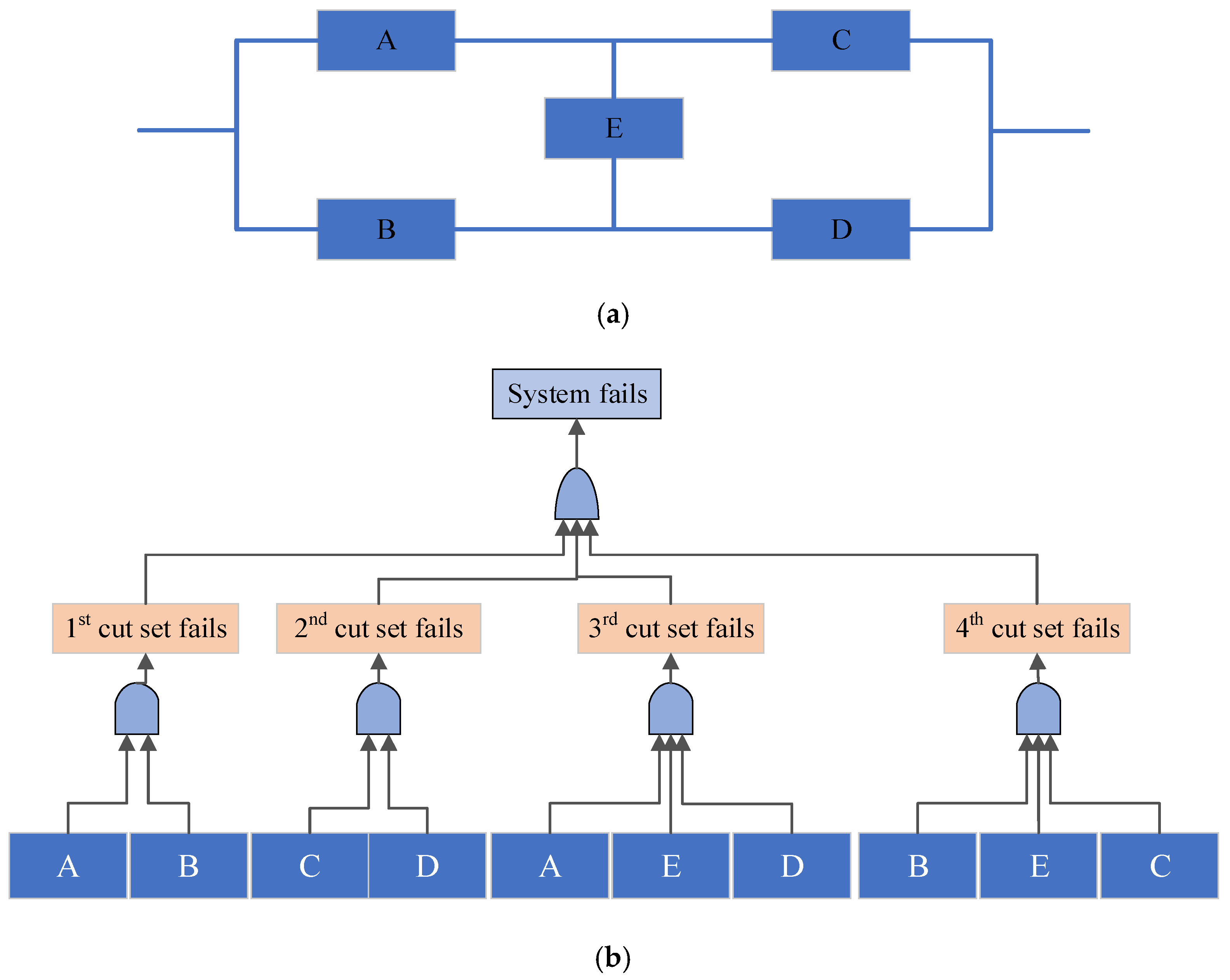
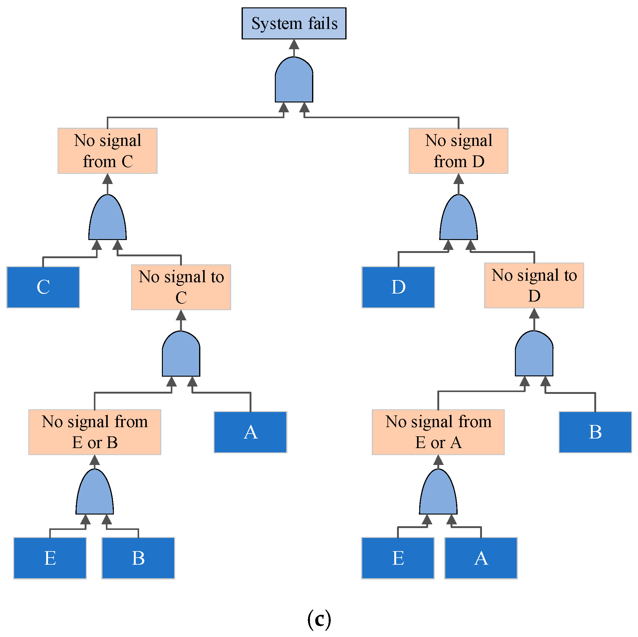
2.2. Basis of Aircraft System Reliability Modeling

The system reliability model in the aviation field currently includes fault trees, reliability block diagrams, event trees, and other methods. To expand the expression and computation ability of these traditional methods, Bayesian networks and Petri nets have also been widely studied in recent years, as shown in Table 1 and Figure 2. These methods describe the fault propagation relationship of the system and its components from different perspectives. Specifically, the fault tree depicts the cause–effect relationship of the fault modes in the system through the logic gate, the reliability block diagram depicts the fault relationship among the components in the system by series, parallel, and hybrid connection and other connections, the event tree describes the possible evolutionary path of various faults in the form of node bifurcation, the Bayesian network describes the causality strength of several types of faults in the system through the node condition probability table, and the Petri net represents the fault propagation process via the tokens flowing between places. See Table 1 for the characteristics of each typical system reliability modeling method.
The essence of these models is to describe the fault propagation paths in the system. Although these methods differ, they rely on experts’ understanding of the system function architecture.
In large-scale complex system reliability modeling, modelers are easily restricted by the level of understanding and analysis. Even if the same model type is used to model the system, the models built by different modelers are likely to differ [33,34]. For example, for a simple system shown in Figure 3a, the fault tree can exist in two forms; see Figure 3b,c. Therefore, only when the reliability model is consistent with the system function architecture as highly as possible can the objective facts of the system be described to the greatest extent to avoid mistakes caused by too many human subjective factors and ensure the correctness of the model.
Otherwise, once the system design specialist completes the function design, the reliability specialist still needs to spend a lot of time and economic cost to build the model, which seriously restricts the progress of the design iteration and leads to the “two-skin” phenomenon, a phenomenon where the work of the system design specialist and reliability specialist is prone to be disjointed, buck-passing, and unable to effectively integrated. This phenomenon is also an important reason affecting aircraft system development progress.
In conclusion, while numerous system reliability modeling techniques exist, they often rely on well-defined system models. Additionally, these methods may require manual intervention or specific expertise to guarantee the accuracy and validity of the resulting reliability models. This creates a significant concern known as the two-skin problem, which slows down the system optimization design process.

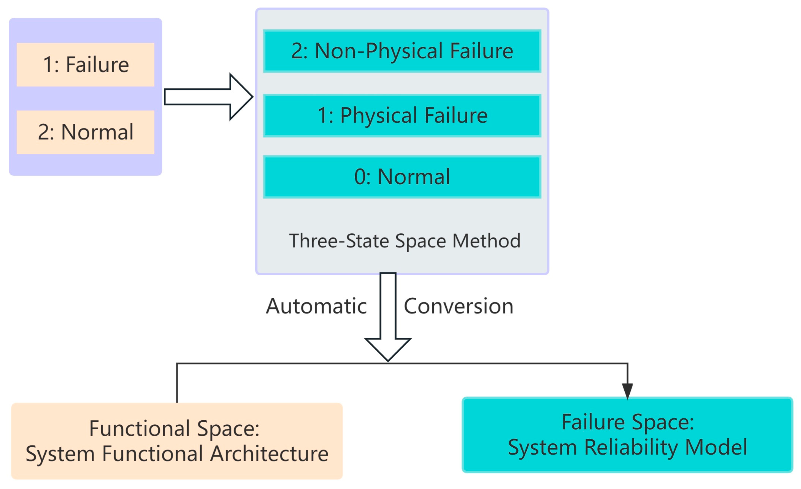
3. The Proposed Three-State Space Modeling Method

The aircraft system design process is an optimization exercise. During this process, the reliability of the system must be modeled and calculated iteratively. One way to speed up the system design optimization process is to address the “two-skin” problem and automatically transform the system architecture into a reliability model, reducing the reliance on expert experience. The key to solving the “two-skin” problem and achieving this automatic transformation lies in moving from the system’s function space to its fault space.
Based on the fault independence assumption commonly used in system reliability analysis, this paper introduces the concept of “Non-physical failure” as a helpful state to connect upstream and downstream nodes in the system function architecture. Then, from a functional perspective, a three-state space modeling method is developed by extending the concept of “Non-physical failure” to introduce a new state called “function loss”. This method automatically transforms the system from its design function architecture (function space) into its reliability model (fault space), as shown in Figure 4.

3.1. Non-Physical Failure State Identified from the Traditional Failure State

On the premise that each component has one single function mode and one single failure mode, each component of the system can be in one of two states: normal (“0”) or fault/failure (“1”). However, in reality, the state of “fault” can be divided into two categories: “Non-physical failure” and physical failure caused by physical damage. “Non-physical failure” refers to a component’s non-working or working abnormally due to error output or no output from its upstream component. In contrast, the component has no physical failure and can work normally.
The state of non-physical failure is widespread in engineering practice and daily life. For example, for a light bulb, the failure of its upstream wires where no current outflows from the wires causes the bulb’s failure to shine even though there is no physical damage. The bulb can normally glow when the upstream wires return to conducting electricity normally. Therefore, the component having upstream components in the system function architecture has three states: the normal, physical failure, and non-physical failure states, represented by 0, 1, and 2, respectively.
Figure 5 is an example to illustrate how to find the local fault propagation path between components in the system function architecture by using the proposed state of non-physical failure.
For the fault-independent system in Figure 5a, the hidden fault propagation path can be described in Figure 5b. In Figure 5a, component G has an AND relationship to C, E, and F. In Figure 5b, 0 represents the normal state, 1 represents the physical failure state, and 2 represents the non-physical failure state. Even though the physical failure of component A is independent of B, the physical failure of A could cause the non-physical failure of B; both the non-physical failure and the physical failure of B could lead to the non-physical failure of C, and both the non-physical and the physical failure state of C could lead to the failure of the subsystem node “Sub-Sys”. Please keep in mind that the nodes that do not correspond to specific components, including the system nodes, subsystem nodes, and other auxiliary nodes, do not have the state of “physical failure” and only have the state of “0” and “2”. In Figure 5, the green line describes the functional propagation, and the red line depicts the fault propagation relationship of the system. Obviously, according to these curves in Figure 5b, it can be seen that the introduction of a non-physical failure state enables the system function architecture to be reasonably explained from both fault and functional perspectives.
In conclusion, the state of non-physical failure is a good way to explain the system function architecture from both the functional and fault perspective; the state is an excellent way to bridge the gap between the system design specialist’s function space and the reliability specialist’s fault space.

3.2. Principles of the Proposed three-State Space Modeling Method

The combined consideration of non-physical failures and the state of physical failures led to the development and explanation of the three-state space modeling method for transforming the system function architecture from the function space to the fault space.
For each component to fulfill its intended function, two preconditions must be met: (i) no physical failure within the component; (ii) no non-physical failure caused by the abnormal operation of upstream components. In the fault perspective, it means that both physical and non-physical failures will result in the loss of function for the component. Additionally, the loss of function in a component is not directly propagated to the system node but gradually to the loss of function in downstream components, ultimately leading to the loss of function in the end component of the system function architecture, which results in the system being non-operational. This is the hidden fault propagation relationship within the system function architecture.
Based on the stated fault propagation relationship within the system function architecture, Figure 6 serves as an example to illustrate the principles of the proposed three-state space modeling method.
In Figure 6a, when A1 experiences a physical failure, it does not directly result in A4, the end component of the system function architecture, being unable to deflect. Rather, it leads to the loss of function in A1: the inability to issue the expected operating instructions. The loss of this function in A1 results in A2 being unable to perform its function of converting the operating instructions from A1 into the expected control command. Additionally, even if A1 were able to issue operating instructions normally, a physical failure in A2 may cause it to fail to correctly convert these instructions into the expected control command. Similarly, the loss of function in A2 and a physical failure in A3 result in A3 being unable to receive the correct control command from A2 or convert these commands into the corresponding analog quantity and actuator position signal to drive the movement of the downstream component. The loss of function in A3 and a physical failure in A4 cause A4 to fail to deflect as expected. When the end component A4 cannot deflect as expected, the system denoted by the node “Sys” is unable to complete its intended function of controlling the aircraft’s flight, indicating a failed or non-functional system.
Based on the aforementioned explanations, Figure 6b presents the hidden fault propagation paths within the function architecture of a system composed of four components. The identification of these hidden paths completes the transformation of the system function architecture from the function space to the fault/failure space.
In addition to the case where downstream components in the system are related to only one upstream component shown in Figure 6, there may also be cases where downstream components are associated with multiple upstream components in a certain logic. For example, the system in Figure 7a expanded based on Figure 6 has several voting logics. In the following, Figure 7 is taken as an example to illustrate the three-state space modeling method for transforming the system architecture, which has general logic gates, such as “Voting”, “AND”, and “OR” from the function space to the fault space.
The system is typically designed in the function space by a design specialist. As such, the logical relationship between a downstream component and its multiple upstream components must be expressed from a functional perspective. For instance, the “2/4 Voting” logic in Figure 7 indicates that among the four upstream components, only when at least two of them can normally output their function can the downstream component perform its function. However, in the fault space, the logical relationship among components in the upstream and downstream is expressed from the perspective of fault propagation path. Therefore, when converting the system architecture to a system reliability model, which is always depicted in the fault space, the functional logic in the architecture must be converted into the equivalent fault logic. This means that the “2/4 Voting” logic in Figure 7b should be converted into the “3/4 Voting” logic in Figure 7c when building a system reliability model. This means that among the four upstream components, only when at least three of them output their function abnormally can the downstream component lose its function. Although the “2/4 Voting” logic in Figure 7b and “3/4 Voting” logic in Figure 7c are depicted from different perspectives, their physical meanings are essentially the same. Similarly, the “AND” and “OR” logic in the function space are equivalent to the “OR” and “AND” logic in the fault space, respectively.
To summarize, when converting the system function architecture to the system reliability model, the logic representing the functional connection relationship between upstream and downstream components needs to be converted into equivalent fault logic through the addition of a third state, “function loss”, which extends from the state of “non-physical” failure.

3.3. Steps of Building the Proposed Three-State Space Model

From the examples in Figure 5, Figure 6 and Figure 7, it can be seen that by dividing the traditional state of failure into physical failure and non-physical failure, the function flow in the system function architecture can be directly converted into the fault propagation paths of the system reliability model without changing the topological structure of the architecture. This transformation completes the shift from the function space to the fault space for the system architecture. Additionally, corresponding to each component/system in the model, the obtained system reliability model contains two types of nodes: type I nodes, which refer to physical failures of components, and type II nodes, which indicate function losses of components/systems.
The method of transforming the system function architecture from the function space to the fault space is defined as the three-state space modeling method, and the three main modeling steps are summarized as follows:
  • List the functions of the system, subsystems, and components the system architecture involves.
  • For each component in the architecture, sort out the function flow in the system function architecture from the following two perspectives.
    • Firstly, suppose that the component itself has no physical failure;
    • Then list the function logic between the component and its upstream components. Generally, the logic among components in the architecture is not drawn in the architecture directly, so the logic should be added to the architecture through logic gates in a clear way.
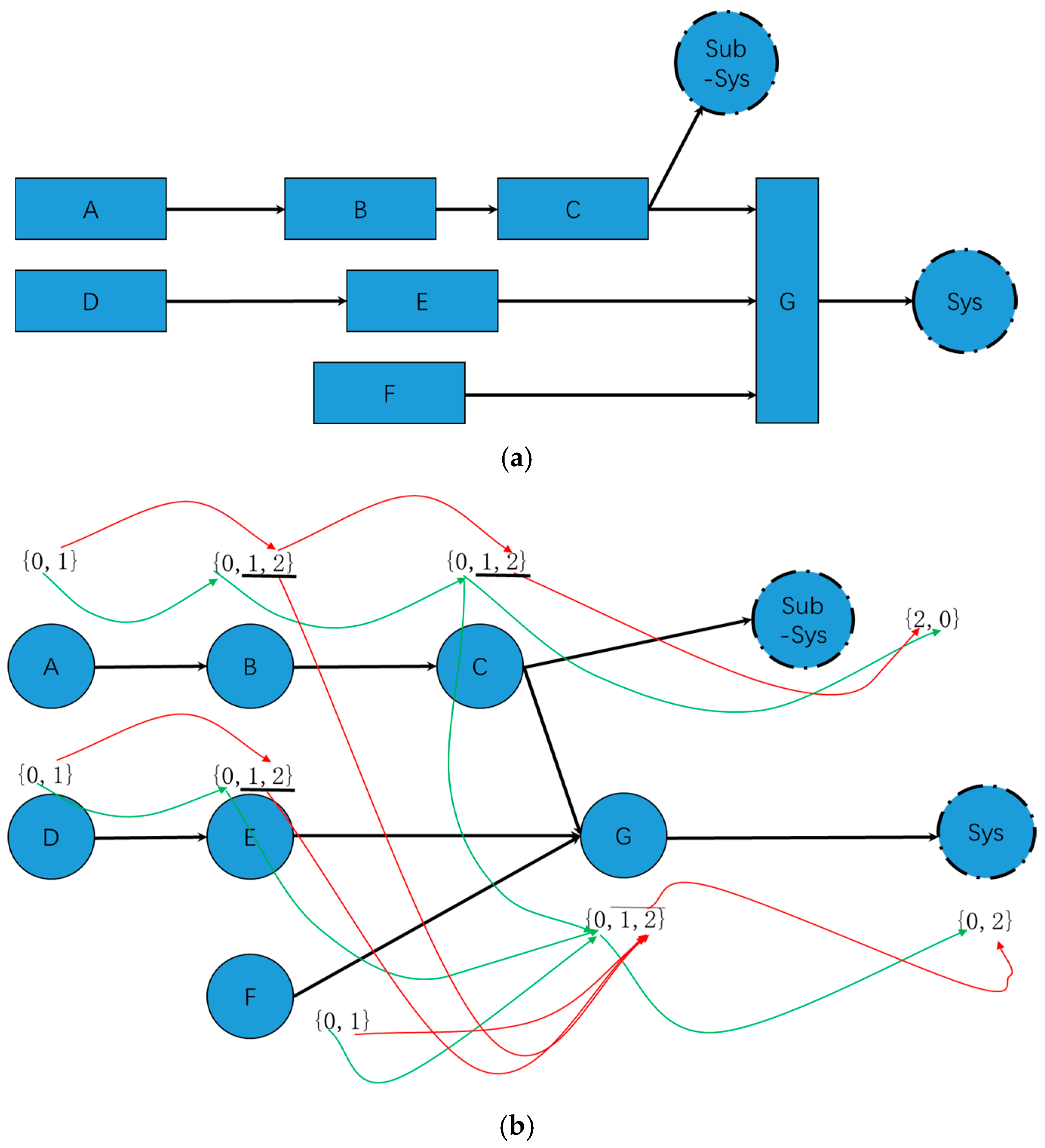
  • Without changing the basic topological structure of the system function architecture, transform the sorted function flow into fault propagation paths in two ways to complete the transformation from the function space to the fault space:
    • Transform component in the non-physical failure state in the function flow of the architecture to the node with physical failure state, that is, the type I node, which is represented as the root node in the topological structure of the system reliability model.
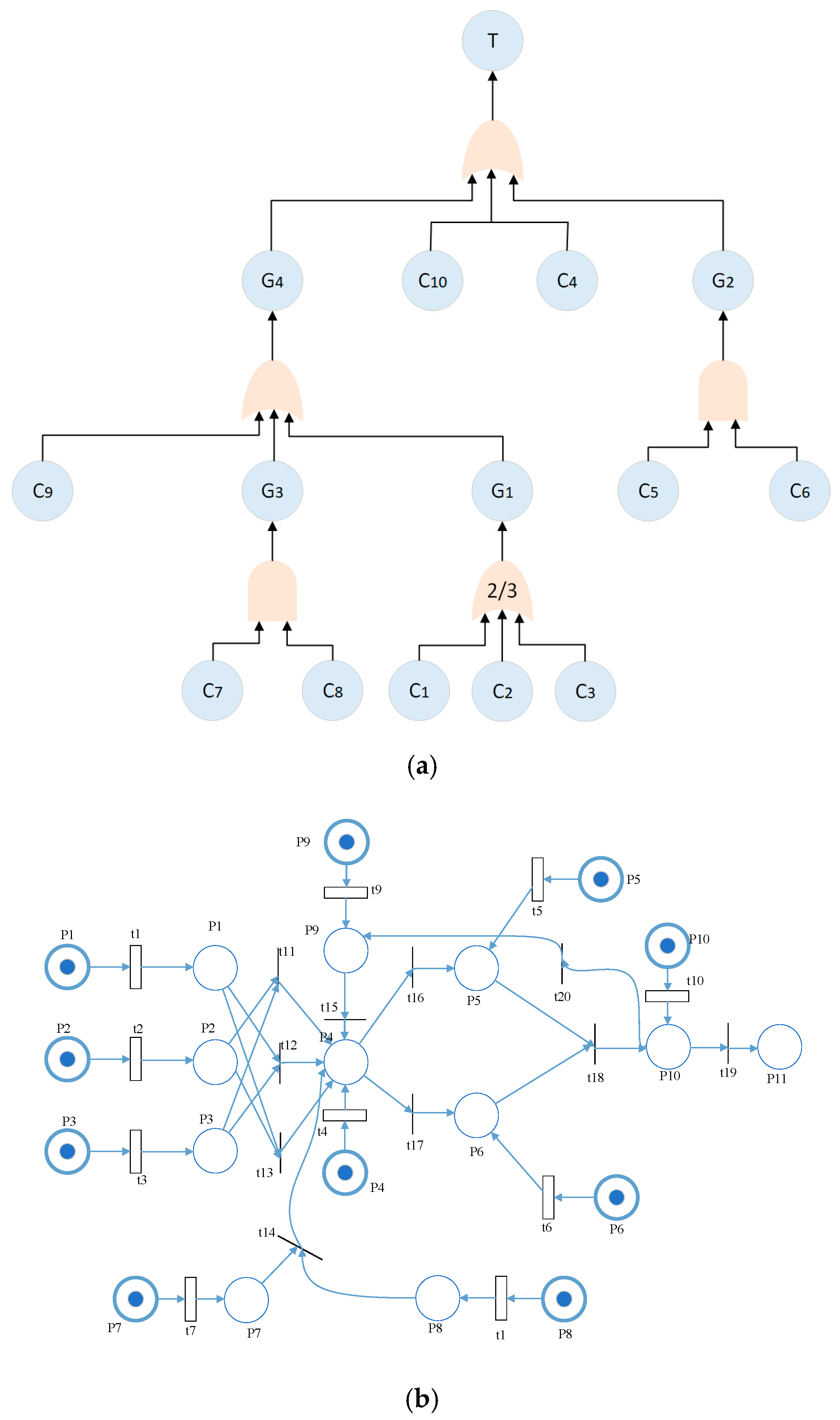
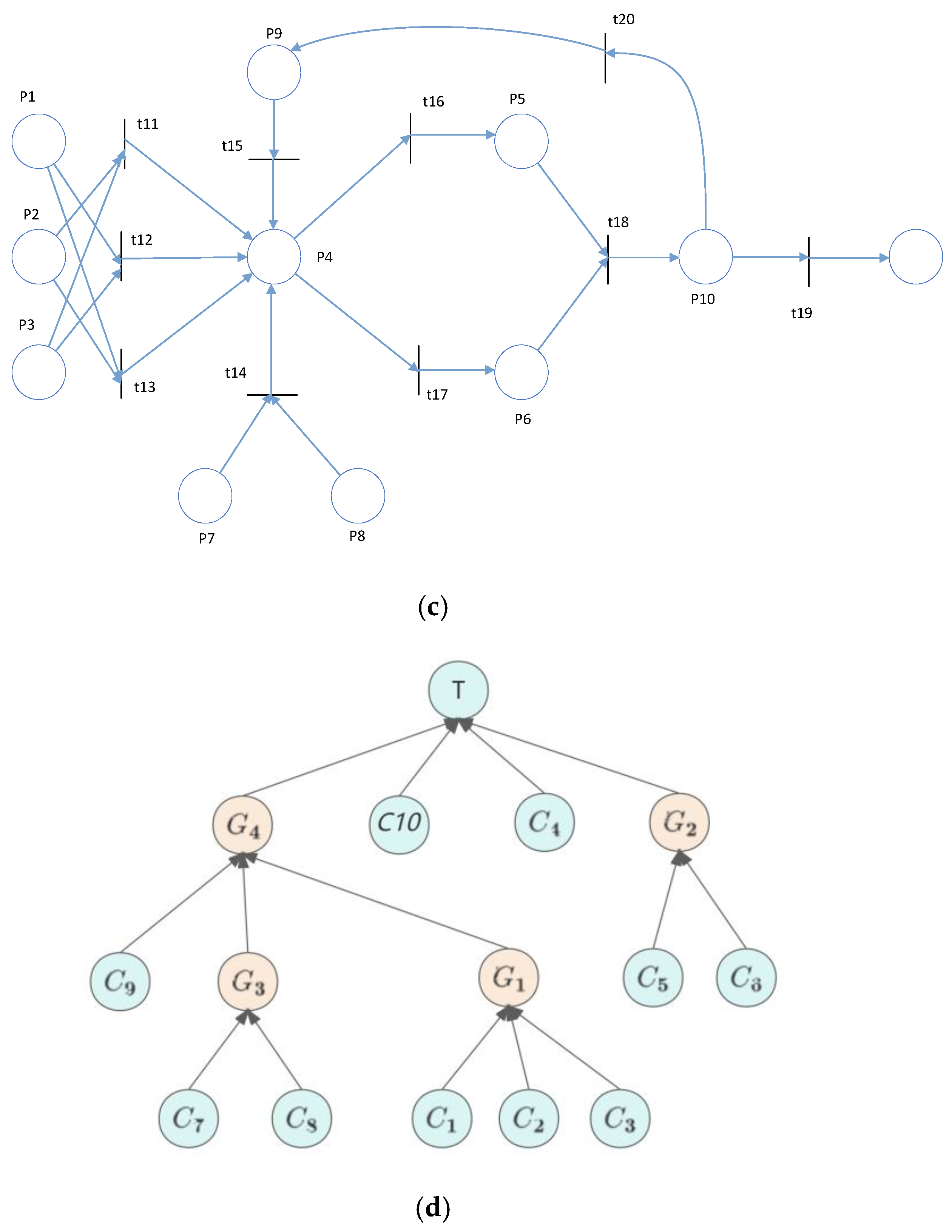
    • According to the converting process from Figure 7b,c, convert nodes representing components’ normal states into nodes representing function loss states. Additionally, convert nodes representing non-physical failure states into nodes representing physical failure states. In this way, type II nodes of the system reliability model are obtained. Additionally, each logic gate expressed from a functional perspective should be converted into its equivalent logic gate with physical meaning from a fault perspective. When a type II node represents a system’s function loss state, it serves as a leaf node in the reliability model and an intermediate node if it represents a component’s function loss.
In summary, this completes the construction of the three-state space model. Furthermore, this model refers to building a model that includes three states: function loss, physical failure, and normal operation.
Finally, for the three-state space model, two points should be noted:
  • Although the modeling method proposed in this paper has one more state than traditional two-state models, modelers still only need to provide failure probabilities or rates of components in the system as inputs for the system reliability model and do not require any additional parameters for the introduced third state of function loss.
  • The modeling method proposed in this paper is not limited to a specific modeling language, so it can be used to construct three-state space models with Petri nets, Bayesian networks, and other modeling languages.

4. Case Studies

The proposed three-state modeling method was performed separately on an aircraft rudder control system and a fly-by-wire control system, using the Bayesian network and the dynamic stochastic Petri net (DSPN) as the modeling languages, respectively. The comparison of the results obtained via the new and traditional methods was used to verify the correctness and effectiveness of the three-state space modeling method.
For the aircraft rudder control system, the three-state space model was constructed using the Bayesian network as the modeling language. The system reliability results were compared with the traditional methods, including FTA, RBD, and the equivalent Bayesian network models of the FTA and RBD. By comparing the results obtained by these methods, we determined whether the three-state space modeling method is correct and effective for the aircraft rudder control system.
For the aircraft fly-by-wire control system, a dynamic stochastic Petri net (DSPN) was used as the modeling language to construct the three-state space model. The system reliability results were compared with the traditional FTA method. By comparing the results obtained by these methods, we determined whether the three-state space modeling method is correct and effective for the aircraft fly-by-wire control system.
Overall, the comparison of the results obtained via the proposed three-state modeling method with traditional reliability modeling methods can verify the correctness and effectiveness of the three-state space modeling method for both aircraft rudder control and fly-by-wire control systems.

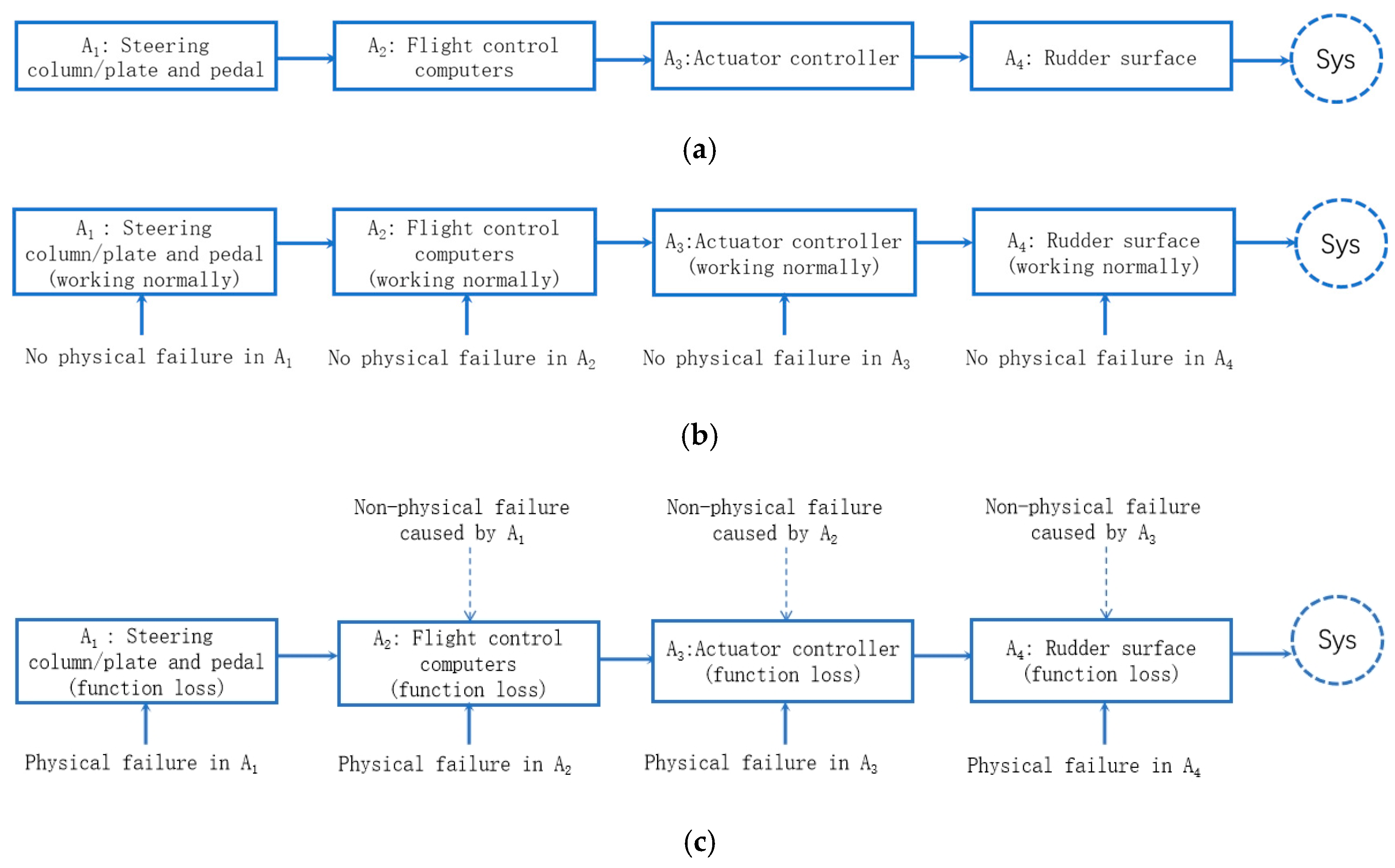
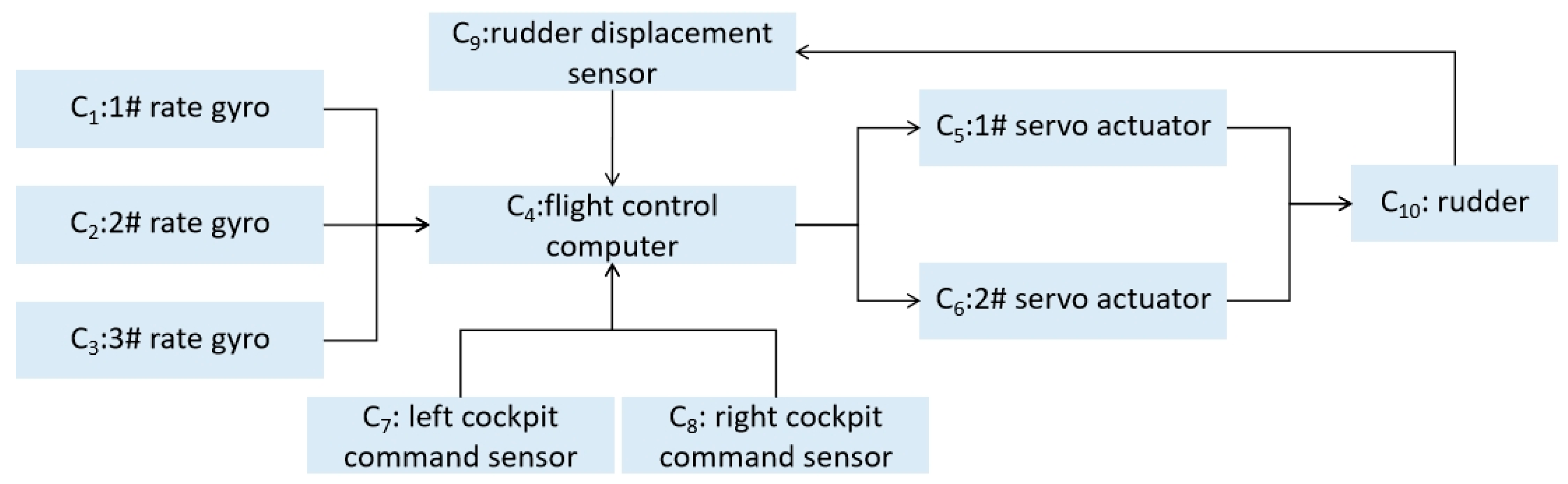
4.1. Reliability Analysis of a Rudder Control System

4.1.1. A Brief Introduction to the Rudder Control System

The aircraft rudder control system in Figure 7 has 11 components: A1 to A11. The pilot can directly operate the components A1 and A2 and pass the operation instructions to the four flight control computers A3A6. After independently solving the operation instructions by converting the operating instructions of A1 and A2 into the expected control command in components A3A6, a “2/4 Voting” logic is performed, which means that the downstream components A7A10 can output their function normally when and only when two of the upstream components A3A6 are in the state of working normally. Then the control commands, after the voting logic is performed, are delivered to actuator controllers A7A10, where the control commands are converted into the analog quantity and the actuator position signal. Similarly, after a “2/4 Voting” logic is performed, the obtained position signal is delivered to the rudder A11 and drives it to deflect as the quantity the pilot wants. The failure probability of all the components in the system at the design stage is supposed to be 0.01.

4.1.2. Reliability Model Construction for the Rudder Control System

The reliability models of the system constructed in different methods are shown in Figure 8. The RBD and FTA modeling methods can be referenced from Refs. [35,36], which are used for the model construction of Figure 8a,c. The conversion method from FTA and RBD to the equivalent BN can be referenced from as Refs. [37,38], which is used to transform the models in Figure 8a,c into the models in Figure 8b,d, separately.
However, as the existing method for assigning the conditional probability table (CPT) of a Bayesian network (BN) is not suitable for reliability models that involve the new state of non-physical failure or function loss, here, the method for assigning CPT for the new proposed three-state space model using a BN as the modeling language is presented as follows:
Firstly, the CPT of each root node can be determined by the failure probability of each component that the root node represents; see Equation (1).
Pr ( X = 1 ) = 0.01 , Pr ( X = 0 ) = 0.99 , X = A 1 , A 2 , A 3 , A 4 , A 5 , A 6 , A 7 , A 8 , A 9 , A 10 , A 11
Secondly, the CPT of the non-root node can be determined based on the proposed three-state space modeling method. The CPTs of the none-root node have two cases, as below. In the following, Y denotes the parent node of Y.
(1)
The physical failure in the parent node Y must lead to the function loss of node Y, after which Pr ( Y = 1 | Y = 1 ) = 1.0 holds; according to the principle of probability normalization, the equation   Pr ( Y = 0 | Y = 1 ) = 1.0 also holds.
(2)
When there is no physical failure in the parent node   Y , the probability of working normally of Y is 1.0, namely Pr ( Y = 0 | Y = 0 ) = 1.0 ; according to the principle of probability normalization, the equation   Pr ( Y = 1 | Y = 0 ) = 0.0 also holds.
Taking nodes A1 and A2 as examples, none of their parents stand for the node having the state of function loss. The CPT tables of nodes A1 and A2 are obtained and shown in Table 2. Similarly, the CPT tables of other nodes in the three-state space model can be obtained.

4.1.3. Reliability Calculation and Discussion for the Rudder Control System

First, four existing techniques were used to perform reliability analysis on the system, including (i) the RBD analysis method for the reliability computation of the RBD model; (ii) the FTA analysis method for the computation of the FTA model; (iii) the Bayesian network inference software SamIam for the computation of RBD’s equivalent BN; and (iv) the software SamIam for the computation of FTA’s equivalent BN model. Secondly, the software SamIam was used to perform reliability analysis on the three-state space model. The results are shown in Table 3. The probability in Table 3 is explained as follows.
As “Sys” represents the system state, system reliability is denoted as Pr (Sys = 0). In the system reliability design process, apart from system reliability, the importance degree as a kind of reliability indicator is also significant for experts to determine the system’s weakness. Based on the weakness, experts can improve the system’s reliability effectively. Moreover, the importance degree can be regarded as an algebraic calculation of two kinds of posterior probability   Pr ( Sys = 1   or   0   | A i = 1   or   0 )   and   Pr ( A i = 1   or   0 | Sys = 1   or   0 ) . For example, the critical importance degree Ic(i) of the component i can be calculated according to Equation (2):
I c ( i ) = Pr ( A i = 1 ) [ Pr ( S y s = 1 | A i = 1 ) Pr ( S y s = 1 | A i = 0 ) ] Pr ( S y s = 1 )
Both Pr ( Sys = 1 | A i = 1 ) and Pr ( Sys = 1 | A i = 0 ) stand for the inference algorithm performed from the component level to the system level in the reliability model; Pr ( A i = 1   | Sys = 1 ) and Pr ( A i = 1   | Sys = 0 ) stand for the inference algorithm performed from the system to the reliability model’s component level.
The results of the three-state space modeling method demonstrate its ability to accurately obtain system reliability results. This method offers several key characteristics that distinguish it from traditional reliability models:
Integration with system architecture: The three-state space model more closely aligns with the system architecture provided by the system design specialist. This alignment eliminates the “two-skin” phenomenon, where the reliability model constructed by the reliability specialist significantly differs from the actual system architecture. By integrating the model with the system architecture, the three-state space model reduces the time and effort required to construct a valid system reliability model, enhancing the collaboration between system design and reliability experts.
Enhanced fault analysis capabilities: The three-state space model not only computes system reliability indicators precisely, but also enhances fault analysis capabilities. This is because the model’s topology structure is highly consistent with the system’s function architecture. This consistency allows for more accurate fault analysis, even when converting RBD and FTA models into equivalent Bayesian networks.
Elimination of expert knowledge dependency: The three-state space model can convert the system into its equivalent reliability model without relying on expert experience. This removes the need for reliability experts to manually construct a valid system reliability model, reducing subjectivity and increasing objectivity in the analysis process.
Early system reliability analysis: The three-state space model has the potential to complete system reliability analysis during the system function design phase. This early analysis provides important guidance to solve the “two-skin” problem between aircraft system design specialists and reliability experts. It allows for the proactive identification of reliability issues and their corresponding solutions, ensuring a more robust and reliable aircraft system design.
In summary, the three-state space modeling method offers a comprehensive and integrated approach to system reliability analysis. It aligns closely with the system architecture, enhances fault analysis capabilities, eliminates expert knowledge dependency, and enables early system reliability analysis. These characteristics make it a promising tool for enhancing collaboration between system design and reliability experts and improving the overall reliability of aircraft systems.

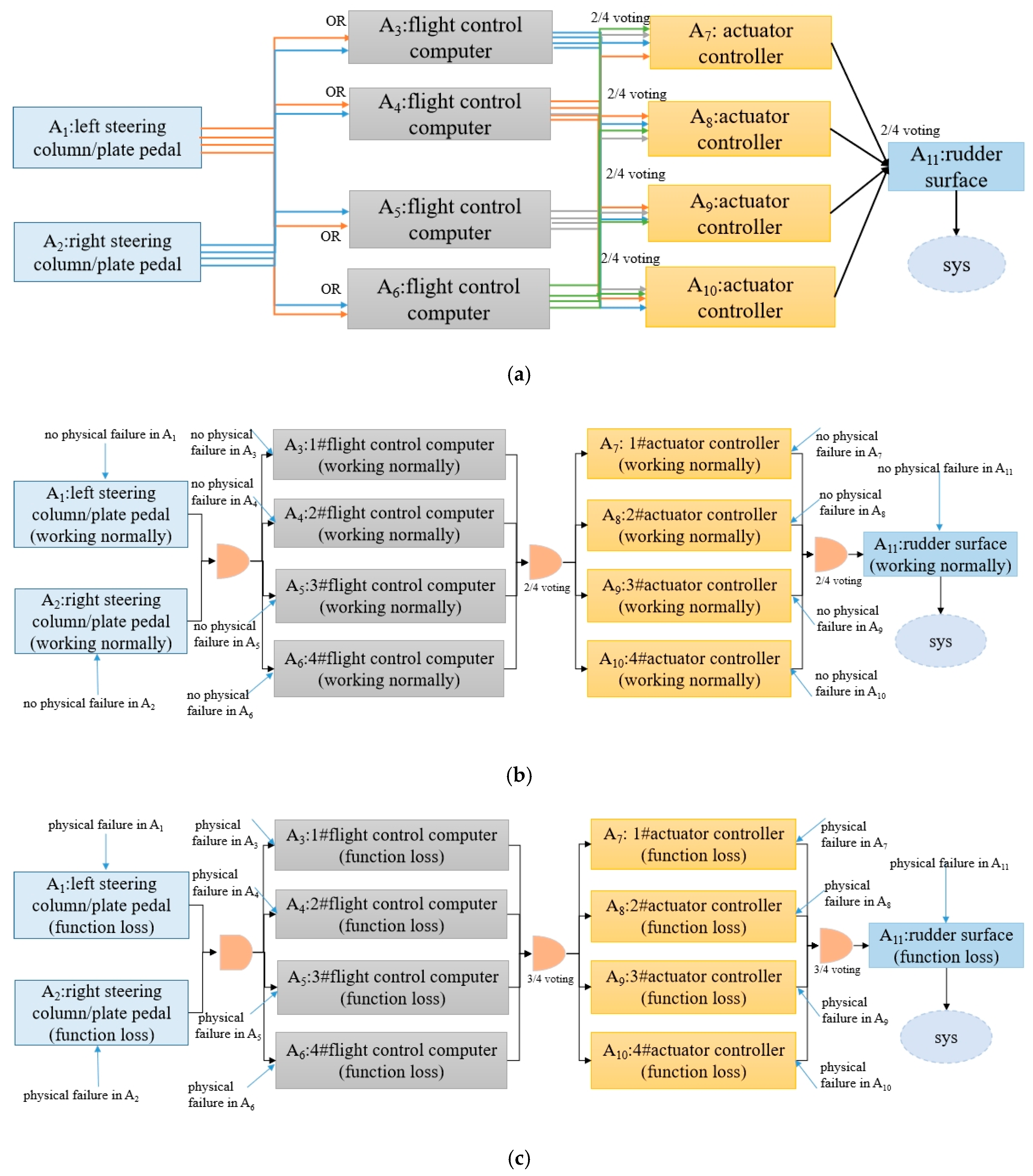
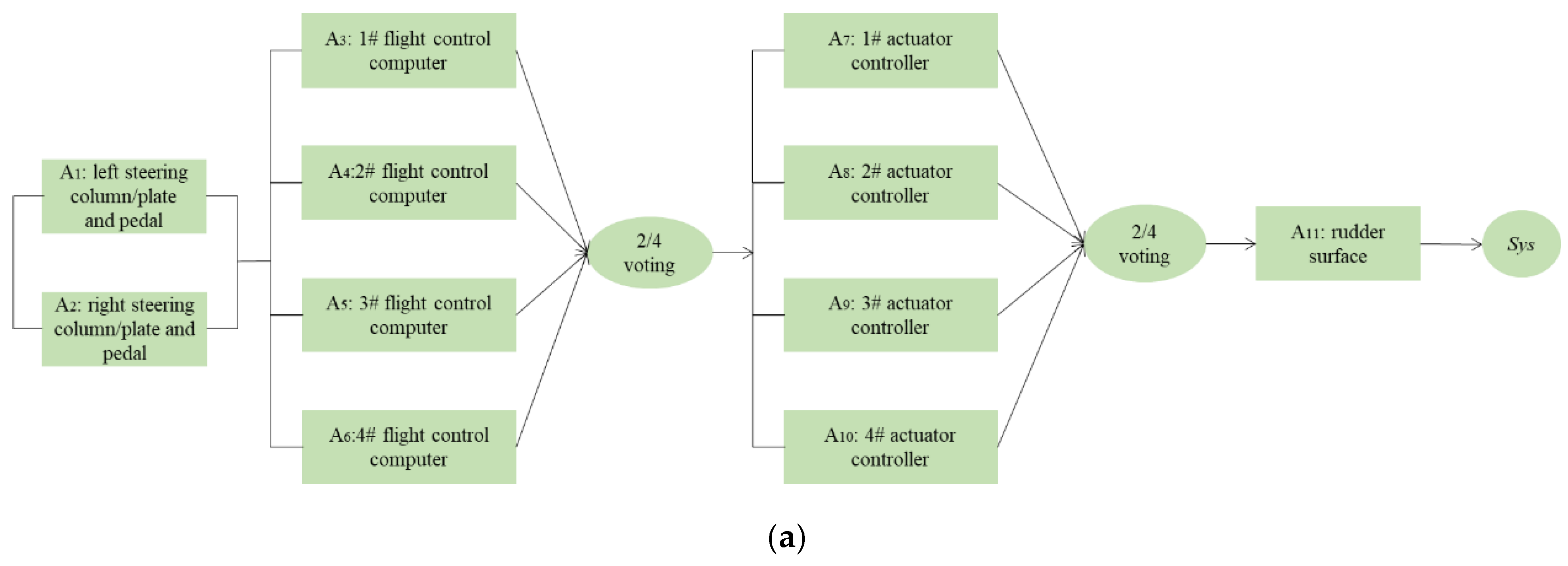
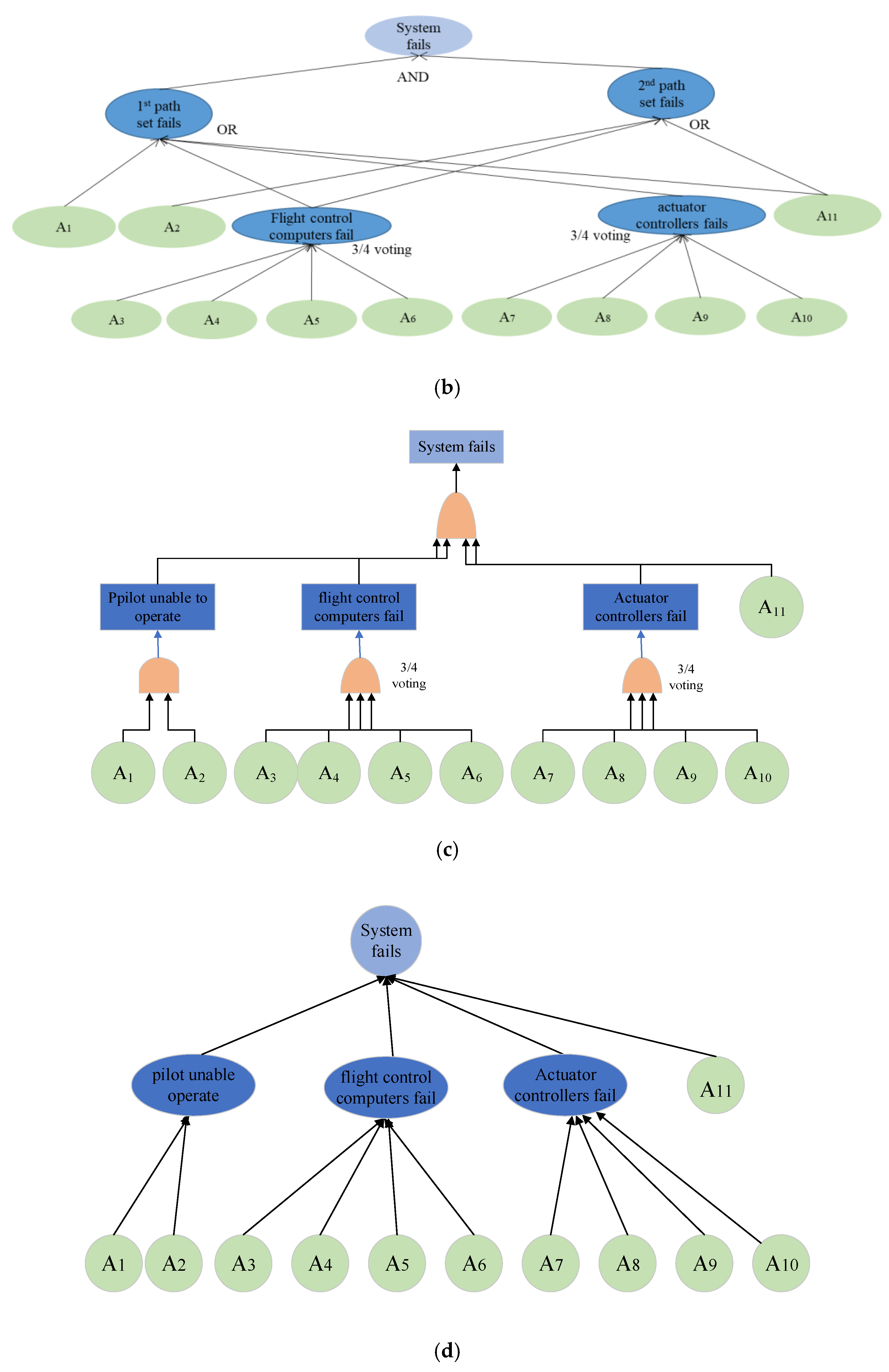
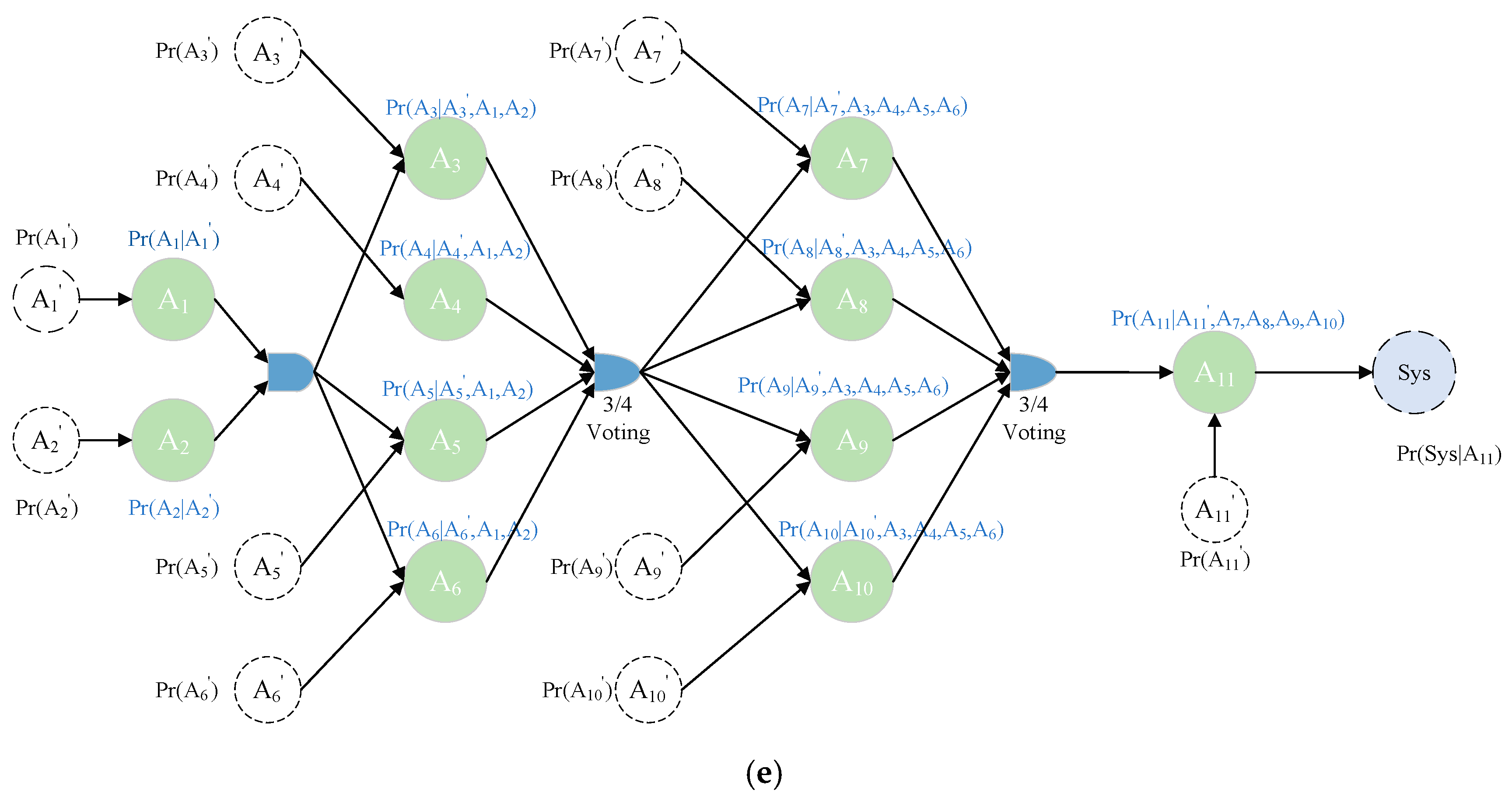
4.2. Reliability Analysis of Aircraft Fly-by-Wire Control System

4.2.1. A Brief Introduction to the Fly-by-Wire Control System

The function architecture of an aircraft flight control system through fly-by-wire technology is depicted in Figure 9. The system consists of ten components: three rate gyros, one flight control computer, two servo actuators, one left cockpit command sensor, one right cockpit command sensor, one rudder displacement sensor, and a rudder surface.
The rate gyros provide rate data to the flight control computer. When at least two of the three rate gyros are functional, the flight control computer can receive this rate data. The pilot’s command instructions are passed to the flight control computer through the command sensors. If the left or right cockpit command sensor is functional, the flight control computer correctly receives the pilot’s command instructions.
Based on the rate data, pilot command instructions, and data from the rudder displacement sensor, the flight control computer calculates effective control signals. These signals are then transmitted to the servo actuators, which drive the rudder to deflect when at least one actuator is functional.
The fly-by-wire control system functions normally if the rudder can deflect normally. Each component within the system has a failure rate associated with it. The failure rates for the rate gyro, flight control computer, servo actuator, cockpit command sensor, rudder displacement sensor, and rudder surface are provided in the figure.
The reliability analysis of such a system requires considering the interactions and dependencies among these components. The three-state space modeling method can be effectively applied to analyze the reliability of this aircraft flight control system, taking into account the system architecture and fault probabilities of each component.
In addition, the failure rate of the rate gyro is 3 × 10⁻⁶, the failure rate of the flight control computer is 5 × 10⁻⁶, the failure rate of the servo actuator is 2 × 10⁻⁶, the failure rate of the cockpit command sensor is 0.7 × 10⁻⁶, the failure rate of the rudder displacement sensor is 0.8 × 10⁻⁶, and the failure rate of the rudder surface is 2 × 10⁻⁶.

4.2.2. Reliability Model Construction for the Fly-by-Wire Control System

The traditional fault tree is used to model the system, as shown in Figure 10a, in which Xi represents the bottom event of the failure of the ith component in the system, G1 represents the intermediate event of the failure of subsystem composed of the three rate gyros, G2 represents the intermediate event of the failure of the subsystem composed of the two servo actuator, G3 represents the intermediate event of the failure of subsystem composed of the two cockpit command sensors, G4 represents the intermediate event that flight control computer receives abnormal data from its neighbor components, and T represents the top event of the system-level failure of the fly-by-wire control system described in this example.
The three-state space model constructed using the proposed method is shown in Figure 10b, where Pi represents the ith component in the system, the bold Pi represents the normal working state of the component, the non-bold Pi represents the failure state of a component, transitions t1-t10 represent the fault evolution process of component i from the normal state to the failure state, and transitions t11t20 represent the fault propagation relationship among components, shown in Figure 10c. These transitions correctly reflect the equivalent transformation of the system from the function space to the failure space. For example, transitions t11, t12, and t13 represent when at least two of the three rate gyros in P1, P2, and P3 fail. The flight control computer cannot receive the aircraft’s rate data, which is consistent with the functional description “When at least two of the three rate gyros are working normally, the flight control computer can receive the aircraft’s rate data”.

4.2.3. Reliability Calculation and Discussion for the Fly-by-Wire Control System

Firstly, the fault tree analysis method calculates the model in Figure 10a. The system reliability R ( τ ) at time τ is calculated as Equations (3)–(7).
R ( τ ) = R ( G 2 ) R ( G 4 ) R 4 R 10
R ( G 2 ) = 1 ( 1 R 5 ) ( 1 R 6 )
R ( G 4 ) = R ( G 1 ) R ( G 3 ) R 9
R ( G 3 ) = 1 ( 1 R 7 ) ( 1 R 8 )
R ( G 1 ) = C 3 2 R 1 2 ( 1 R 1 ) + R 1 3 )
Ri denotes the reliability of the ith component in the system. Let λ i denotes the failure rate of component i, then Equation (8) holds.
R i = e λ i τ ,   i = 1 , 2 , 3 , 4 , 5 , 6
The system’s reliability at system time τ = 100, 200⋯3000 is calculated based on these equations obtained from fault tree analysis. The result obtained using this fault tree analysis method is given in the second column of Table 4 and given as the exact solution in Figure 11.
Secondly, as the fault tree can be converted into an equivalent Bayesian network, here the model in Figure 10d is converted to the Bayesian network for calculating the system reliability, see the BN in Figure 10d. The result obtained using this BN method is given in the third column of Table 4 and given as the exact solution in Figure 11.
Thirdly, the Monte Carlo analysis method is performed on the proposed three-state space model in Figure 10b. Based on the simulation method, the system’s reliability at time τ can be calculated as Equation (9):
R ( τ ) = 1 S i m n = 1 S i m N δ S i m N                 δ = { 1                           i f   S Y S [ S i m _ n ] τ 0                             i f   S Y S [ S i m _ n ] > τ }
SimN is the simulation times, and the array SYS[SimN] records the failure time of the system in each simulation process, where Sim_n = 1, 2…SimN. The results obtained using the three-state space model in GSPN language with Monte Carlo simulation at SimN = 1000, 50,000 and 100,000 are given in the fourth-sixth column of Table 4, and the results at different SimN are also given in Figure 11.
The calculation results obtained from the traditional fault tree model and the proposed three-state space model are shown in Figure 11 and Table 4.
The results are discussed as follows.
Compared with traditional modeling methods, the three-state space modeling method proposed in this paper exhibits high consistency with the system function architecture, providing excellent manipulability for modelers. This means that a system reliability model can be quickly constructed during the modeling process, with minimal reliance on expert experience and effort.
The manipulability of the model is closely linked to its representation method. A representation method that mirrors the system’s physical structure and function architecture usually offers superior manipulability. By comparing Figure 9 with Figure 10c and Figure 9 with Figure 10a, it is evident that the topology structure of the reliability model obtained through the proposed three-state space modeling method aligns closely with the system function architecture, whereas the fault tree model derived through traditional modeling methods exhibits significant deviations from the system function architecture.
The proposed three-state space modeling method ensures more thorough retention of system working principle information, leading to a more objective representation of the system in the system reliability modeling process.
Upon comparing the topological structures of Figure 9 and Figure 10c, it becomes evident that these two structures are completely consistent. This implies that the model represented in Figure 10c, constructed using the proposed three-state modeling method, accurately preserves the system working principle information encoded in Figure 9. This eliminates the need for system reliability modelers to reinterpret the system designers’ intentions regarding the system working principle, leading to a more objective system description during the reliability modeling process. This effectively mitigates errors associated with traditional modeling methods that rely heavily on human expertise.
Moreover, the proposed modeling approach is effective for conducting system reliability calculations.
The three-state space modeling method is employed to model the fly-by-wire control system using the generalized stochastic Petri nets (GSPNs) language. Monte Carlo simulation is an effective technique for evaluating GSPN models. Therefore, Monte Carlo simulations were conducted on the GSPN to estimate system reliability at various system times. According to the law of large numbers, as the number of simulations, Sim_N, increases, the reliability estimate obtained through Monte Carlo converges towards the true solution. As depicted in Figure 11, it is evident that as the number of simulations increases, the reliability computed using the method proposed in this study stabilized at its true value.
Furthermore, the simulation count significantly impacts the accuracy of system reliability estimates. To address this, this paper presents a method for determining an acceptable simulation count. Initially, an initial simulation count of SimN = 1000 was established. Once this count is reached, reliability statistics can be gathered.
Step1. An initial simulation number SimN = 1000 was set. After SimN = 1000 is reached, system reliability can be obtained by statistics.
Step2. The simulation count was incremented from SimN = 1000 to SimN = 2000. This involves performing an additional 1000 simulations on the GSPN model. After these new simulations conclude, the system reliability can be updated by combining the results from Step 1 with those from the new simulations.
Step3. If the reliability results from Steps 1 and 2 were closely aligned and fell within an acceptable error range, the reliability results were considered converged, and there is no need to increase the simulation count further. Alternatively, if the reliability results from Steps 1 and 2 deviate significantly, the simulation count was incremented in increments of 1000 (e.g., SimN = 3000, SimN = 4000, etc.) until the reliability results obtained at SimN and SimN + 1000 were consistent.
In summary, the proposed three-state space modeling method not only transforms the system function architecture at the system design stage into a reliability analysis model, but also computes system reliability efficiently. These features ensure that reliability analysts can effectively complete system reliability assessments once the system designers provide a functional architecture. This eliminates the “two-skin” problem between aircraft system designers and reliability analysts, enhancing the efficiency of system development.

5. Conclusions

The three-state space modeling method proposed in this paper can effectively address the “two-skin” phenomenon between the reliability specialist and the system design specialist. By dividing failures into “physical failure” and “non-physical failure” and introducing the third state of “function loss” into the reliability modeling process, the method fully retains the system working principle information and avoids the reliability specialist having to reprocess the system designers’ intention about the system working principle. This makes the aircraft system reliability optimization process accelerated.
The three-state space modeling method is adaptable for engineers who prefer different modeling languages during system reliability optimization work. After the modeling language is selected, the proposed model could be constructed, and then engineers can directly use the existing calculation methods or tools for calculating the system reliability results. In this way, the calculation difficulty for engineers can be reduced, and thus the optimization process also could be accelerated.
The proposed three-state space model is highly consistent with the system function architecture. It fully reflects the advantages of combining function and failure modes in one model. Thus, it enables the reliability specialist to respond timely to the function design of the system design specialist and has the great potential to solve the “two-skin” phenomenon between the two specialties, which is of great significance in improving the reliability optimization efficiency of aircraft system development.
In summary, the proposed three-state space model is a promising method for addressing the “two-skin” phenomenon between the reliability specialist and the system design specialist. It can effectively improve the efficiency of aircraft system reliability optimization and is of great significance in aircraft system development.
To solve the problem of the “two-skin” phenomenon between the reliability specialist and the system design specialist and speed up the aircraft system reliability optimization process, this paper firstly divides failures into “physical failure” and “non-physical failure”, then proposes “function loss” as the new state of a system in addition to the traditional state of “normal” and “fault”. Based on the new state, a three-state space modeling method for constructing a system reliability model was developed that makes the reliability specialist transform the system function architecture provided by the system design specialist into a system reliability model directly without much relying on expert experience and effort, making the system reliability optimization process accelerated. Finally, the proposed modeling method was applied to one rudder control system and one fly-by-wire control system, and the results show that.

6. Patents

Part of this research work was patented by the Patent Office of the People’s Republic of China:
Wang Y, Sun Q. A reliability analysis method for aircraft fly-by-wire control system. China: ZL 201610969751.3, 14 February 2020.

Author Contributions

Conceptualization, Y.W.; methodology, Y.W.; software, Y.F.; validation, F.W., and S.C.; formal analysis, Y.F.; investigation, F.W.; resources, S.C.; data curation, F.W.; writing—original draft preparation, Y.W.; writing—review and editing, S.C.; visualization, Y.F.; supervision, F.W.; funding acquisition, S.C. and Y.W. All authors have read and agreed to the published version of the manuscript.

Funding

This research was funded by the Aviation Industry Corporation of China Limited, Grant/Award Number: ASFC-202300130T6003, the National Natural Science Foundation of China, Grant/Award Number: 12102346.

Data Availability Statement

Data are contained within the article. The data presented in this study are available in Section 4 of the article.

Acknowledgments

The first author would like to thank Xiaomin Hu, whose valuable comments helped the quality of this work improve significantly.

Conflicts of Interest

The authors declare no conflict of interest.

References

  1. Moir, I.; Seabridge, A. Aircraft Systems: Mechanical, Electrical, and Avionics Subsystems Integration; John Wiley & Sons: Hoboken, NJ, USA, 2011. [Google Scholar]
  2. Guo, W. Analysis of Maintenance Cost of B737NG Aircraft. Available online: https://www.sohu.com/a/358383293_651535 (accessed on 12 October 2023).
  3. Society of Automotive Engineers Aerospace. Guidelines for Development of Civil Aircraft and Systems; SAE: Warrendale, PA, USA, 2010. [Google Scholar]
  4. Tiassou, K.; Kanoun, K.; Kaâniche, M.; Seguin, C.; Papadopoulos, C. Aircraft operational reliability—A model-based approach and a case study. Reliab. Eng. Syst. Saf. 2013, 120, 163–176. [Google Scholar] [CrossRef]
  5. Blatnický, M.; Dižo, J.; Sága, M.; Molnár, D.; Slíva, A. Utilizing Dynamic Analysis in the Complex Design of an Unconventional Three-Wheeled Vehicle with Enhancing Cornering Safety. Machines 2023, 11, 842. [Google Scholar] [CrossRef]
  6. Song, L.K.; Bai, G.C.; Fei, C.W.; Tang, W.Z. Multi-failure probabilistic design for turbine bladed disks using neural network regression with distributed collaborative strategy, Aerosp. Sci. Technol. 2019, 92, 464–477. [Google Scholar]
  7. Zio, E.; Fan, M.; Zeng, Z.; Kang, R. Application of reliability technologies in civil aviation: Lessons learnt and perspectives. Chin. J. Aeronaut. 2019, 32, 143–158. [Google Scholar] [CrossRef]
  8. Coit, D.W.; Zio, E. The evolution of system reliability optimization. Reliab. Eng. Syst. Saf. 2019, 192, 106259. [Google Scholar] [CrossRef]
  9. Zhou, C.; Chang, Q.; Zhao, H.; Ji, M.; Shi, Z. Fault tree analysis with interval uncertainty: A case study of the aircraft flap mechanism. IEEE T. Reliab. 2020, 70, 944–956. [Google Scholar] [CrossRef]
  10. Kornecki, A.; Liu, M. Fault Tree Analysis for Safety/Security Verification in Aviation Software. Electronics 2013, 2, 41–56. [Google Scholar] [CrossRef]
  11. Xu, Q.; Xu, Y.; Tu, P.; Zhao, T.; Wang, P. Systematic Reliability Modeling and Evaluation for On-Board Power Systems of More Electric Aircrafts. IEEE T. Power Syst. 2019, 34, 3264–3273. [Google Scholar] [CrossRef]
  12. Xiong, L.; Fan, Y.; Liu, Y.; Yang, Z.; Zeng, Z. Reliability analysis of service routing for a power system communication network based on MCS-RBD. IEEJ T. Electr. ELectr. 2018, 13, 1642–1648. [Google Scholar] [CrossRef]
  13. Anes, V.; Morgado, T.; Abreu, A.; Calado, J.; Reis, L. Updating the FMEA Approach with Mitigation Assessment Capabilities—A Case Study of Aircraft Maintenance Repairs. Appl. Sci. 2022, 12, 11407. [Google Scholar] [CrossRef]
  14. Ivančan, J.; Lisjak, D.; Pavletić, D.; Kolar, D. Improvement of Failure Mode and Effects Analysis Using Fuzzy and Adaptive Neuro-Fuzzy Inference System. Machines 2023, 11, 739. [Google Scholar] [CrossRef]
  15. Shiao, M.; Chen, T.K. Probabilistic Risk Assessment Tool AMETA (Aircraft Maintenance Event Tree Analysis) for Aircraft Structural Integrity and Fatigue Maintenance. In Proceedings of the AIAA SciTech 2019 Forum, San Diego, CA, USA, 7–11 January 2019. [Google Scholar]
  16. Lawhorn, D.; Rallabandi, V.; Ionel, D.M. Scalable graph theory approach for electric aircraft power system optimization. In Proceedings of the 2019 AIAA/IEEE Electric Aircraft Technologies Symposium (EATS), Indianapolis, IN, USA, 22–24 August 2019. [Google Scholar]
  17. Kumar, T.B.; Sekhar, O.C.; Ramamoorty, M. Composite power system reliability evaluation using modified minimal cut set approach. Alex. Eng. J. 2018, 57, 2521–2528. [Google Scholar] [CrossRef]
  18. Nobakhti, A.; Raissi, S.; Damghani, K.K.; Soltani, R. Dynamic reliability assessment of a complex recovery system using fault tree, fuzzy inference and discrete event simulation. Eksploat. Niezawodn. 2021, 4, 593–604. [Google Scholar] [CrossRef]
  19. Mueller, S.; Gerndt, A.; Noll, T. Synthesizing Failure Detection, Isolation, and Recovery Strategies from Nondeterministic Dynamic Fault Trees. J. Aeros. Comp. Inf. Com. 2019, 16, 52–60. [Google Scholar] [CrossRef]
  20. Swanke, J.A.; Jahns, T.M. Reliability Analysis of a Fault-Tolerant Integrated Modular Motor Drive for an Urban Air Mobility Aircraft Using Markov Chains. IEEE T. Transp. Electr. 2022, 8, 4523–4533. [Google Scholar] [CrossRef]
  21. Bayrak, G.; Acar, E. Reliability Estimation Using Markov Chain Monte Carlo–Based Tail Modeling. AIAA J. 2017, 56, 1211–1224. [Google Scholar] [CrossRef]
  22. Zhao, Y.; Che, Y.; Lin, T.; Wang, C.; Liu, J.; Xu, J.; Zhou, J. Minimal cut sets-based reliability evaluation of the more electric aircraft power system. Math. Probl. Eng. 2018, 2018, 9461823. [Google Scholar] [CrossRef]
  23. Zhang, Q.; Wang, L.; Rong, H.; Gu, Q.; Zhang, R. A Dynamic Fault Tree Analysis Method Based on Discrete-time Bayesian Network for the Core Processing System of IMA. In Proceedings of the 2020 IEEE 11th International Conference on Software Engineering and Service Science (ICSESS), Cairo, Egypt, 16–18 October 2020. [Google Scholar]
  24. Wang, Y.; Yang, M.; Miao, Z.; Dong, X. A Reliability Modelling Method for Aircraft Electrical Power System Based on Probability Network. In Proceedings of the International Conference on Mathematics and Computers in Sciences and Industry (MCSI), Corfu, Greece, 25–27 August 2018. [Google Scholar]
  25. Guo, P. Research on the reliability analysis method of the complex aircraft system based on the Petri nets. Adv. Aeronaut. Sci. Eng. 2016, 7, 174–180. (In Chinese) [Google Scholar]
  26. Menu, J.; Nicolai, M.; Zeller, M. Designing fail-safe architectures for aircraft electrical power systems. In Proceedings of the 2018 AIAA/IEEE Electric Aircraft Technologies Symposium (EATS), Cincinnati, OH, USA, 12–14 July 2018. [Google Scholar]
  27. Hoz, C.; Bussemaker, J.H.; Fioriti, M.; Boggero, L.; Nagel, B. Environmental and Flight Control System Architecture Optimization from a Family Concept Design Perspective. In Proceedings of the AIAA Aviation Forum, Virtual, 15–19 June 2020. [Google Scholar]
  28. Zio, E. Reliability engineering: Old problems and new challenges. Reliab. Eng. Syst. Saf. 2009, 94, 125–141. [Google Scholar] [CrossRef]
  29. Zhang, Y.; Kurtoglu, T.; Tumer, I.Y.; O’Halloran, B. System-Level Reliability Analysis for Conceptual Design of Electrical Power Systems. In Proceedings of the Conference on Systems Engineering Research (CSER), Redondo Beach, CA, USA, 15–16 April 2011. [Google Scholar]
  30. Joshi, A.; Heimdahl, M.P.E.; Miller, S.P.; Whalen, M.W. Model-Based Safety Analysis; No. NASA/CR-2006-213953; National Aeronautics and Space Administration, Langley Research Center: Hampton, VA, USA, 2006. [Google Scholar]
  31. Barker, T.; Parnell, G.S.; Pohl, E.; Specking, E.; Goerger, S.R.; Buchanan, R.K. Impact of Reliability in Conceptual Design—An Illustrative Trade-Off Analysis. Systems 2022, 10, 227. [Google Scholar] [CrossRef]
  32. Diatte, K.; O’Halloran, B.; Van Bossuyt, D.L. The Integration of Reliability, Availability, and Maintainability into Model-Based Systems Engineering. Systems 2022, 10, 101. [Google Scholar] [CrossRef]
  33. Wang, Y.; Gao, X.; Cai, Y.; Yang, M.; Li, S.; Li, Y. Reliability evaluation for aviation electric power system in consideration of uncertainty. Energies 2020, 13, 1175. [Google Scholar] [CrossRef]
  34. Kritzinger, D. Aircraft System Safety: Military and Civil Aeronautical Application; Woodhead Publishing: Cambridge, UK, 2006. [Google Scholar]
  35. Modarres, M.; Kaminskiy, M.P.; Krivtsov, V. Reliability Engineering and Risk Analysis: A Practical Guide, 3rd ed.; CRC Press: Boca Raton, FL, USA, 2016. [Google Scholar]
  36. Elsayed, E.A. Reliability Engineering; John Wiley & Sons: Hoboken, NJ, USA, 2012. [Google Scholar]
  37. Khakzad, N.; Khan, F.; Amyotte, P. Safety analysis in process facilities: Comparison of fault tree and Bayesian network approaches. Reliab. Eng. Syst. Saf. 2011, 96, 925–932. [Google Scholar] [CrossRef]
  38. Kim, M.C. Reliability block diagram with general gates and its application to system reliability analysis. Ann. Nucl. Energy 2011, 38, 2456–2461. [Google Scholar] [CrossRef]
Figure 1. Aircraft system reliability optimization process during design.
Machines 12 00013 g001
Figure 2. System reliability modeling in the system design stage.
Machines 12 00013 g002
Figure 3. Bridge-linked system and its two equivalent fault trees. (a) Function architecture of the bridge-linked system; (b) the first equivalent fault tree for the bridge-linked system; (c) the second equivalent fault tree for the bridge-linked system.
Machines 12 00013 g003aMachines 12 00013 g003b
Figure 4. The role of the three-state space method in transforming system function architecture into system reliability modeling.
Machines 12 00013 g004
Figure 5. A multi-input system and its equivalent three-state space model. (a) The function architecture of a multi-input system; (b) the equivalent three-state space model, which depicts the fault propagation paths.
Machines 12 00013 g005
Figure 6. Transformation of one rudder control system from the function space to the fault space. (a) Function architecture of one simple aircraft rudder control system; (b) function flow in the function architecture; (c) fault propagation path hidden in the function architecture.
Machines 12 00013 g006
Figure 7. Conversion of one complex rudder control system from the function space to the fault space. (a) Function architecture of one more complex aircraft rudder control system; (b) function flow in a more complex function architecture; (c) fault propagation path hidden in a more complex function architecture.
Machines 12 00013 g007
Figure 8. Five equivalent models of a rudder control system. (a) RBD model of the system; (b) BN model converted from RBD; (c) FTA model of the system; (d) BN model converted from FTA; (e) the proposed three-state space model described in a Bayesian network modeling language.
Machines 12 00013 g008aMachines 12 00013 g008bMachines 12 00013 g008c
Figure 9. Function architecture of an aircraft fly-by-wire control system.
Machines 12 00013 g009
Figure 10. Two types of reliability models for the aircraft fly-by-wire control system. (a) Fault tree model of the system; (b) three-state space model described in the modeling language of GSPN; (c) the fault propagation path described in the three-state space model. (d) BN model converted from FTA.
Machines 12 00013 g010aMachines 12 00013 g010b
Figure 11. Reliability results of the aircraft fly-by-wire control system.
Machines 12 00013 g011
Table 1. Summary of system reliability modeling methods.
System ModelsModel StructureInput Parameters of the ModelThe Output of the ModelThe Way of Modeling Computing Ability
FTATree structure consisting of basic events, intermediate events, and top eventsFixed failure rates of componentsSystem reliability, structural importance, probabilistic importance, etc.Relying on expert experienceInvolving Boolean disjoint operations and combinatoric explosion problems
RBDComposite for series, parallel, etc.System reliabilityRelying on expert experienceInvolving Boolean disjoint operations and combinatoric explosion problems
ETBranch structureSystem reliability, consequences of component failureRelying on expert experienceInvolving Boolean disjoint operations
FMEAThe form of a table Severity level of failure modes Relying on expert experienceUnable to perform quantitative calculations
BNDirected acyclic graph with multiple nodesSystem reliability, structural importance, probabilistic importance, Bayesian importance, etc.Transformed from FTA, RBD, FEMA Boolean disjoint operations are avoided and have a superior computational ability than FTA and RBD
Petri netA graph consisting of places, tokens, directed flows, and transitions System reliabilityTransformed from FTA, RBD, FMEAHaving the ability of visualization of fault propagation with the help of Monte Carlo simulation
Table 2. Table of conditional probabilities for nodes A1 and A2 (Y = A1, A2).
Y′      YPr(Y|Y′)
0      01.0
0      10.0
1      00.0
1      11.0
Table 3. Calculation results of the rudder control system under different modeling methods1.
RBD Analysis MethodFTA MethodBN Reasoning Technique
RBD ModelFTA ModelBN Converted from RBDBN Converted from FTAThe Proposed Three-State Space Model
Pr(Sys = 0)0.9898930.9898930.9898930.9898930.989893
Pr(A1 = 1|Sys = 1)0.0196970.0196970.019697
Pr(A2 = 1|Sys = 1)0.0196970.0196970.019697
Pr(A3 = 1|Sys = 1)0.0102880.0102880.010288
Pr(A4 = 1|Sys = 1)0.0102880.0102880.010288
Pr(A5 = 1|Sys = 1)0.0102880.0102880.010288
Pr(A6 = 1|Sys = 1)0.0102880.0102880.010288
Pr(A7 = 1|Sys = 1)0.0102880.0102880.010288
Pr(A8 = 1|Sys = 1)0.0102880.0102880.010288
Pr(A9 = 1|Sys = 1)0.0102880.0102880.010288
Pr(A10 = 1|Sys = 1)0.0102880.0102880.010288
Pr(A11 = 1|Sys = 1)0.9894270.9894270.989427
Pr(Sys = 1|A1 = 1)0.0199080.0199080.0199080.0199080.019908
Pr(Sys = 1| A2 = 1)0.0199080.0199080.0199080.0199080.019908
Pr(Sys = 1|A3 = 1)0.0103980.0103980.0103980.0103980.010398
Pr(Sys = 1|A4 = 1)0.0103980.0103980.0103980.0103980.010398
Pr(Sys = 1|A5 = 1)0.0103980.0103980.0103980.0103980.010398
Pr(Sys = 1|A6 = 1)0.0103980.0103980.0103980.0103980.010398
Pr(Sys = 1|A7 = 1)0.0103980.0103980.0103980.0103980.010398
Pr(Sys = 1|A8 = 1)0.0103980.0103980.0103980.0103980.010398
Pr(Sys = 1|A9 = 1)0.0103980.0103980.0103980.0103980.010398
Pr(Sys = 1|A10 = 1)0.0103980.0103980.0103980.0103980.010398
Pr(Sys = 1|A11 = 1)11111
Note: In system failure/reliability analysis, indicators are usually represented as the prior probability and the posterior probability. The results of solving the prior and posterior probability problems using the five methods are given in the table, where “/” means unsolvable.
Table 4. Calculation results of the fly-by-wire control system under different methods.
System TimeFTA MethodBN Converted
from FTA
Three-State Space Method in GSPN Language simN = 1000 Three-State Space Method in GSPN Language
simN = 50,000
Three-State Space Method in GSPN Language
simN = 100,000
2000.998440 0.998440 0.998000 0.998000 0.998000
4000.996880 0.996880 0.999950 0.997675 0.996000
6000.995320 0.995320 0.994000 0.995500 0.995000
8000.993759 0.993759 0.996000 0.996500 0.993000
10000.992199 0.992199 0.996000 0.993900 0.992000
12000.990639 0.990639 0.990000 0.990240 0.990500
14000.989079 0.989079 0.994000 0.991600 0.989000
16000.987519 0.987519 0.994000 0.990600 0.987000
18000.985958 0.985958 0.982000 0.984240 0.986500
20000.984398 0.984398 0.990000 0.987340 0.984700
22000.982838 0.982838 0.986000 0.984700 0.983200
24000.981278 0.981278 0.976000 0.978840 0.981700
26000.979718 0.979718 0.990000 0.985000 0.979800
28000.978158 0.978158 0.996000 0.987360 0.978700
30000.976599 0.976599 0.974000 0.975200 0.977000
Disclaimer/Publisher’s Note: The statements, opinions and data contained in all publications are solely those of the individual author(s) and contributor(s) and not of MDPI and/or the editor(s). MDPI and/or the editor(s) disclaim responsibility for any injury to people or property resulting from any ideas, methods, instructions or products referred to in the content.

