Trajectory Generator System for a UR5 Collaborative Robot in 2D and 3D Surfaces

Abstract

In Industry 4.0., robots are regarded as one of the key components. In recent years, collaborative robots (cobots) have risen in relevance and have been included in the industry to perform tasks alongside humans. Robots have been used in many applications in manufacturing processes; for the scope of this paper, the emphasis on these applications is centered on welding and gluing. These applications need to be performed with specific speed, efficiency, and accuracy to attain optimal welding or bonding to the pieces. An operator cannot maintain such conditions consistently, with minimum variations, for an extended period; hence, robots are a more suitable option to perform those tasks. The robots used for these applications need to be instructed to follow a trajectory to either weld or apply the glue. This path must be programmed on the robot by an operator, and depending on the complexity of the trajectory, it can take up to extended periods of time to set all the required waypoints. There are specialized software environments that contribute to the automation of these tasks; however, the overall cost of the licenses is not affordable if the scale of the project only requires developing and programming trajectories a few times. This paper contains a proposal for an open-source Computer Aided Manufacturing (CAM) software to automatically generate the trajectories needed for the aforementioned welding and gluing applications. The procedure to develop the software starts by selecting the surface that will be welded or to which glue will be applied. The surface determines the model of the trajectory to be followed. Next, a processing system is fed with the individual points that make up the trajectory provided by their selection over the Computer Aided Drawing (CAD) model. This system then creates a program based on URScript^® that can be directly uploaded to and executed on the robot. A set of tests is presented to validate the applications and to demonstrate the versatility of the developed trajectory generation system.

1. Introduction

In the field of robotics, there are as many definitions of what a robot is as there are types of robots. For the purpose of this paper, the definition given by Peter Corke will be used: “a robot is a goal-oriented machine that can sense, plan and act” [1]. In this research, the focus will be on serial manipulator collaborative robots. As mentioned in [2], collaborative robots, also known as cobots, are designed to work side by side with human operators. They offer fewer barriers than other types of robots to their use in automation projects, such as lower cost, high versatility, almost plug-and-play installation and no need for a cage (in most applications) without sacrificing safety, thanks to their force-limited joints.

News outlets love to picture automation as a job-stealing evil and turn it into a battle of humans vs. machines, but the reality could not be farther from the truth. Humans and machines are better working as a team, and as a team, every member has their strengths and weaknesses. There are some tasks that humans are not well prepared to execute, which is where robots come in. The guideline for the 4Ds of robotization states which tasks should be automated by a robot: Dull, Dirty, Dangerous and Dear [3].

• Dull: The task is repetitive or tedious;
• Dirty: The task or the environment where it is developed is unpleasant;
• Dangerous: The task or the environment represents a security risk;
• Dear: The task is expensive or critical.

The 4D guideline not only aids in deciding if a task is suitable for its robotization, but it also highlights how robots can contribute to the value chain. “Overall, robots increase productivity and competitiveness. Used effectively, they enable companies to become or remain competitive. This is particularly important for small to medium-sized enterprises (SMEs) that are the backbone of both developed and developing country economies. It also enables large companies to increase their competitiveness through faster product development and delivery”, as stated by The International Federation of Robotics (IFR) in its annual global report on industrial robotics in 2022 [4]. It is worth noting that robots not only have economic advantages, but they also provide operational advantages, such as “increase of manufacturing productivity (faster cycle time) and/or yield (less scrap), improved worker safety, reduction of work-in-progress, greater flexibility in the manufacturing process and reduction of costs” [4].

As previously mentioned, robotics has a huge impact on the industry and can be especially beneficial for small to medium-sized enterprises (SMEs). For SMEs to be able to leverage the full capabilities of a robot, they would need to overcome some obstacles, such as lack of experience with automation [5], lack of a widely adopted standardized robotic programming language [6], high cost for entry [7] and even fear of robots taking over [8]. In this project, we attempt to reduce the barrier for entry into robotics for SMEs, reducing the learning curve and eliminating the cost of a Computer Aided Manufacturing (CAM) software by developing an open-source CAM Software with simple functionalities to trace and simulate robot trajectory with the Computer Aided Drawing (CAD) model of the workpiece and generate the program for the robot.

The task to be automated is trajectory waypoint capturing. As the first step of this task, an operator uses a cobot in collaborative mode to place the end effect in the desired waypoint of the trajectory in the workpiece surface. Secondly, the operator saves the waypoint and moves the end effector to the next waypoint. This process is repeated as many times as needed to complete the whole trajectory. This type of task is executed for adhesive bonding and arc welding applications.

Robotic arms help to achieve a faster and more accurate weld path while keeping the operators safe from the spark and toxic fumes. Suppliers of the automotive industry not only need to deliver high-quality jobs efficiently, but they must also be flexible in the requirements of the clients and the specifications of different value chains. The implementation of robots makes possible the creation of complex weld paths in a short amount of time and reduces costs [9].

Robotic Adhesive Bonding, also known as Robotic Gluing, is being used by suppliers of the automotive industry to seal GPS antennas and tanks in the vehicle body. The robot can spread the adhesive bead evenly while ensuring an accurate fit on the workpiece, which improves quality, reduces cycle time and reduces unit cost [10].

The improvement of trajectory planning for robotic manipulators is a relevant topic in the current state of the automation research community, as can be seen in [11,12,13,14,15]. An application to develop a smooth joint path is presented in [11]. This paper focuses on the optimization of the trajectories of the robot. In [12], the movement of a worker is used to create a predictive model, which generates the path considering obstacle avoidance. There are applications that try using obstacle avoidance on a robot path; for example, in [13], the authors present an algorithm to obtain an optimal solution to the trajectory of the robot to avoid an obstacle. The result presented by the authors is a set of waypoints that the user needs to insert manually into a robot program. In [14], a configuration plane is used to present an obstacle avoidance algorithm; the method provides an inverse kinematics solver to present a smooth trajectory to perform the task. In [15], the vibration of robots is presented as a problem to be solved, so the authors proposed a practical implementation strategy to reduce the vibrations using a delay finite response filter to implement a time-varying input shaping technology.

As presented in [11,12,13,14,15], trajectory generation and optimization represent an area of opportunity for improvement in robotics. This paper aims to contribute to this research by describing a method to create trajectories based on a CAD model path. Another one of the objectives of this project was to stay on the grounds of user-friendly platforms, for which reason the default simulator and programmer of Universal Robots (UR)Polyscope were selected.

Additionally, contrary to the process shown in [3,4,5], in which an operator loads the program to the robot based on the waypoint coordinates, the system described in this paper uses a parser that translates the selected coordinates into a file in the proprietary programming language URScript^® [16] to automate the process. This feature proves invaluable when more intricate trajectories require a large number of points to perform a certain task.

2. Materials and Methods

The programs used in the project are SolidWorks 2021 from Dassault Systèmes, MATLAB from MathWorks, Python and Polyscope from UR. The software were used in that order to create our system.

SolidWorks was used to model the workpiece whose surface would have the 3D trajectory and to export the CAD model to Standard Triangle Language (STL) format. As a clarification, SolidWorks was used because the developing team had university licenses active. The heavy lifting was done by MATLAB and Python; a high-end CAD program was not needed for the usage of this system.

The main tools used in the development of this system were the numeric computing platform MATLAB, due to its simulation capabilities and its development environment, and the available Toolboxes of Robotics, Image Processing and Partial Differential Equations, which sped up the prototyping and testing process. MATLAB was used for CAD model processing, image processing, to turn a CAD model into an interactive user interface, trajectory information extraction from the user interface, robot trajectory generation and simulation of the manipulator robot following the 2D Trajectory of an image or 3D trajectory in the surface of the CAD model of the workpiece.

The Python programming language was used due to its versatility and efficiency insofar as text manipulation and file generation are concerned. It was also chosen thanks to its compatibility with the file formats that were chosen throughout the development of the project.

The system performs three main tasks to generate a trajectory that can be executed by the robot. The first task consisted of determining the path itself, depending on the type of surface over which the trajectory would be generated. For 3D surfaces, an interactive interface was used, in which the user can choose different points that will make up the main path. For 2D surfaces, which allow the generation of more complex trajectories, an image processing algorithm was used to determine the edges of a figure uploaded as a JPG image. In both cases, the points were interconnected, and the positions and orientations for the created path of the end effector were subsequently calculated.

The second task was the simulation of the generated trajectory to ensure the feasibility of the provided points and orientation. Using a digital representation of both the robot and the surface in which the path would be traced, a simulation of the movements needed to complete the trajectory was displayed to the user. If the path was feasible within the physical limitations of the robot, parameters that determine the necessary information for the simulation, such as the type of movement, the position, the orientation, and the configuration space it must adopt in each waypoint, were recorded and exported as a Comma Separated Value (CSV) file.

The third task consisted of transforming the values contained in the CSV file into a programming language that could be understood by the robot. This was accomplished by a parsing algorithm that translated the provided parameters into executable commands, considering both the type of movement and the configuration space in which the robot was situated. The resulting list of commands was saved as a script that could be directly uploaded into the robot for its execution.

Using MATLAB 2022a and Python 3.8, we created a free and easier open-source alternative to enterprise CAM software for welding and glue applications.

2.1. Theoretical Framework

2.1.1. Collaborative Robots

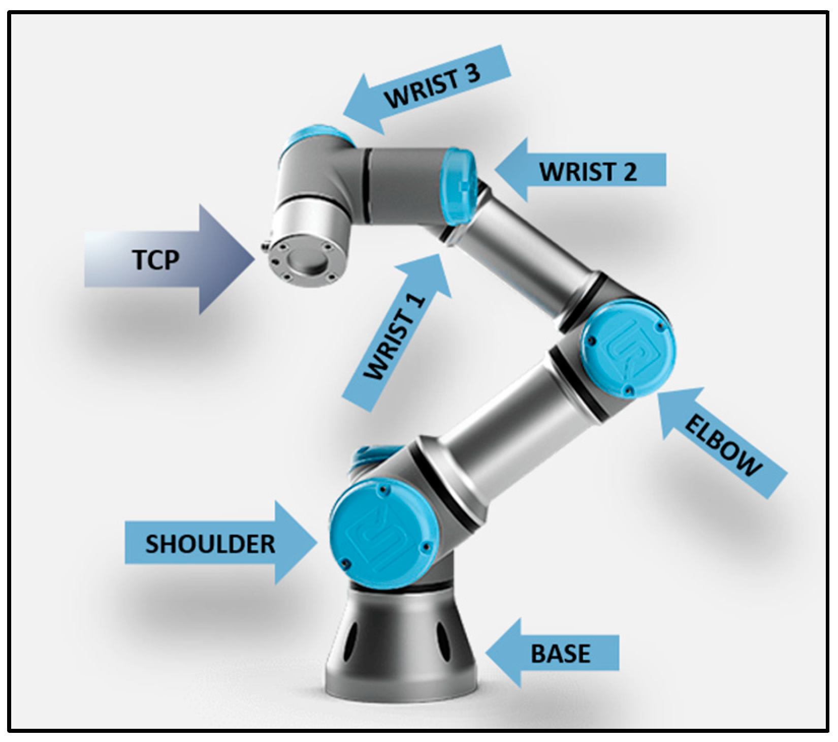
The focus of this paper is on serial manipulator robots, which have the shape of a robotic arm, as the one shown in Figure 1. The objective of a manipulator robot is to reach the desired position and orientation with whatever end effector they have attached. A common modelling and analysis technique for robotic movements is to consider the end effector as a single point, called Tool Center Point (TCP).

The system described in this paper was developed for collaborative robots, commonly referred to as cobots. The main feature of this type of robotic manipulator is their capability to share their workspace with a human worker without posing grave risks for the operators they work alongside. To maintain this quality, collaborative robots are built with a lightweight structure and a sensible collision detection control system. Their movements are relatively slow as well, with the aim of not posing a security threat to the objects and humans in their shared workspace.

2.1.2. Programming Types

There are two ways to program a collaborative robot: manual programming and script-oriented programming.

In manual programming, a human operator uses a Graphic User Interface (GUI) to program a robot by concatenating blocks that contain individual commands. Each individual point in the trajectory can be specified using waypoints, which is a structure containing the position and orientation values of the cobot at that specific point. As the operator has the possibility of physically interacting with the robot, these values can be manually adjusted.

For simple applications that need a trajectory consisting of around 25 waypoints, manual programming is a sensible approach. However, when the application is more complex, and the quantity of waypoints are in the order of the hundreds or thousands, a different technique is needed.

Script programming uses the programming language of the robot to generate commands not as blocks with individual values but as lines of code in which the position and orientation, the type of movement, and the configuration space of the robot are specified. As the name indicates, script programming uses individual scripts, or files, that contain the required trajectory and series of movements. This file is then uploaded into the robot to be executed by it. These scripts can be automatically created by code generators.

2.1.3. Trajectory Generator Systems

There are professional software tools used to generate a trajectory on the surface of a CAD model. This is only one of their many functionalities, as they are programming environments with a great variety of applications.

One of the most popular professional software tools is RoboDK. This programming environment allows the user to import any CAD model, automatically generate the desired trajectory for different applications, simulate the proposed movement and generate a ready-to-upload file in the programming language of a physical robot. It is compatible with most commercial robots, and its capability to generate programs for any of the selected robots is a great factor in its widespread use and popularity [17].

Another professional software that is relevant in modern settings is Process Simulate, created by the automation and infrastructure company Siemens. This programming environment offers many manufacturing solutions and integration with a great portion of other Siemens products. Among its functionality catalog, it allows the simulation of robots for a myriad of applications. One such application is for Trajectory planning for welding applications [18].

These professional programming environments are quite useful but require a huge economic investment, the amount of features can be overwhelming, and the numerous training required for operators and developers.

2.2. Project Proposal

To generate a trajectory that can be executable for the robot, the system starts by determining the path, which has slight variations depending on the type of trajectory to be generated and its characteristics.

Figure 2 describes as a block diagram the flow for the case of 3D trajectories, and the process starts with a CAD model of the piece on whose surface the path will be traced. The model to be imported into MATLAB is used to generate a mesh over which the user can select different nodes to create the desired trajectory. The position and orientation that the TCP of the robot must take to traverse these selected points are then calculated using inverse kinematics. From here onwards, a position and orientation pair will be referred to as a pose, which is a mathematical structure that comprises position and orientation to use in linear transformations.

Figure 3 describes the same, but in the case of 2D trajectories, the main difference is that all paths are configured to be traced on a flat surface. Since the additional adjustments for the 3D surface can be disregarded, the complexity of the trajectories can increase. To explore the possibility, an image processing algorithm was used to transform JPG images into trajectories by identifying the outline of the figures and mapping them to analyzable points. These points are saved as a .mat file and then mapped to poses acquired by the robot as it follows the trajectory.

As a way of preliminary testing, a simulation is run, where a digital model of the robot follows the selected trajectory over the provided surface. Such trajectory can either come from the CAD model for 3D paths or from the .mat file for its 2D counterpart. If the simulation does not have the desired outcome, user-selected parameters, such as the speed of the TCP, initial robot configuration, the number of frames used in the simulation, and the position and orientation of the TCP relative to the workpiece and the trajectory, can be modified. Once the simulation gives the desired result, several parameters, such as the configuration space of the robot, the type of movement, and the pose values acquired throughout the different points in the trajectory, are saved as a CSV file.

Afterwards, through a Graphical User Interface, the CSV file is uploaded into a parsing algorithm developed in Python. This program stores the trajectory poses that were extracted from the CSV file in objects. These objects are used to generate and concatenate the strings for the different movement functions. The result is a script ready to be executed by the robot.

2.3. Transform a CAD Model into an Interactive Trajectory Selector

In this section, the procedure to obtain an Interactive Trajectory Selector from a CAD model is presented. The process requires different steps to implement the solution and is divided into the following steps:

• Converting a CAD Model into a Mesh;
• Using a Mesh as the foundation for an Interactive Trajectory Selector;

In the following paragraphs, there is a detailed explanation of each step to understand the whole process.

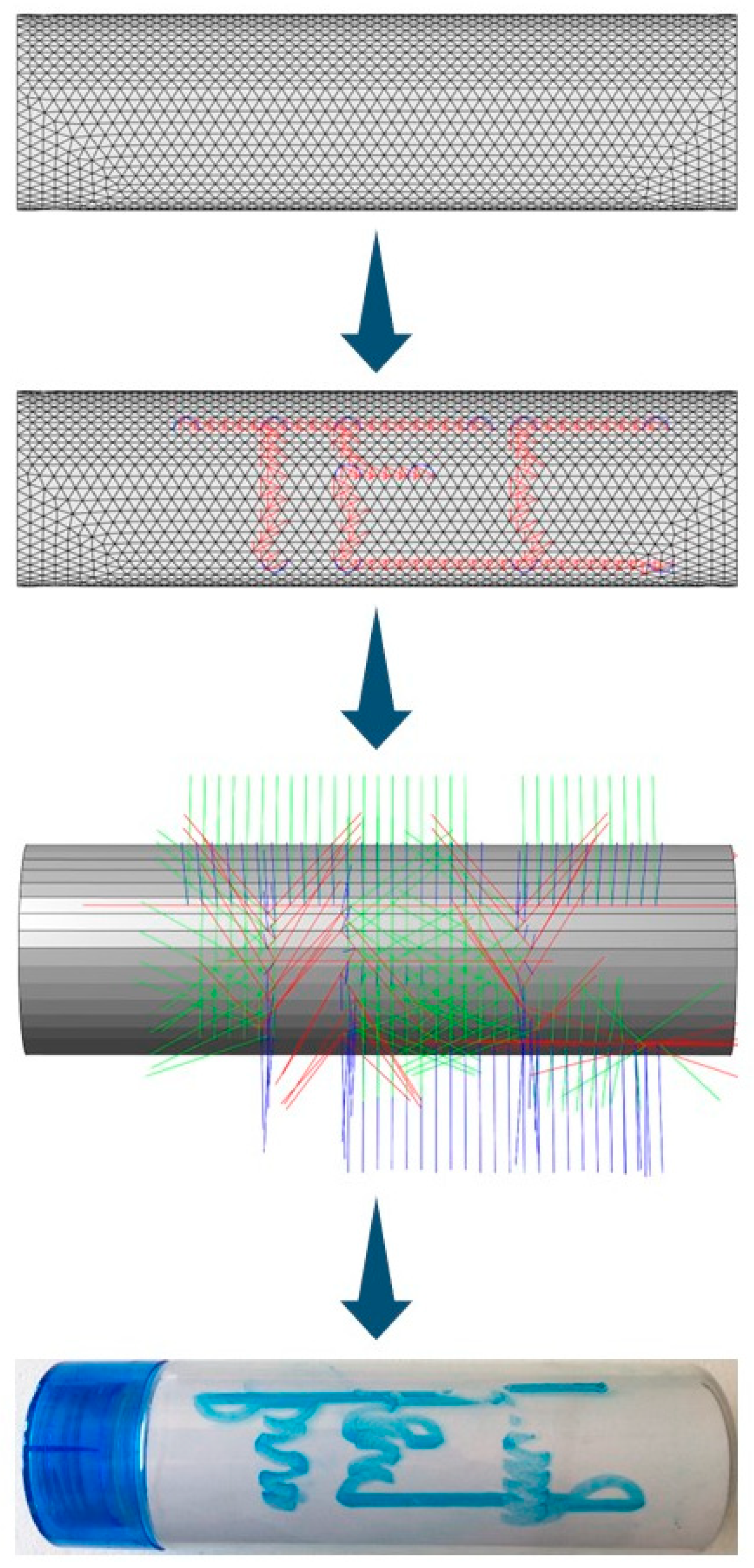
2.3.1. Converting a CAD Model into a Mesh

The generation of a trajectory over a 3D surface requires the CAD model of the piece over which the path will be traced. It must then be imported into MATLAB, a programming platform, in which the piece undergoes three steps to become the mesh used for the Interactive Trajectory Selector.

The first step is to save the original CAD model in a STL file format. The second step is to import the CAD model in STL format to MATLAB; the model is imported as a Discrete Geometric Model (DGM). The third and final step is to convert the DGM into a mesh. The Partial Differential Equation (PDE) Toolbox [19] enables the importing of the CAD model in STL format as a DGM and the conversation from DGM to mesh.

Figure 4 provides a visual representation of the transformation from CAD model to mesh. From left to right, the original CAD Model, the STL format CAD Model, the DGM, and the mesh. The original piece for this CAD model was a regular cylinder.

2.3.2. Using a Mesh as the Foundation for an Interactive Trajectory Selector

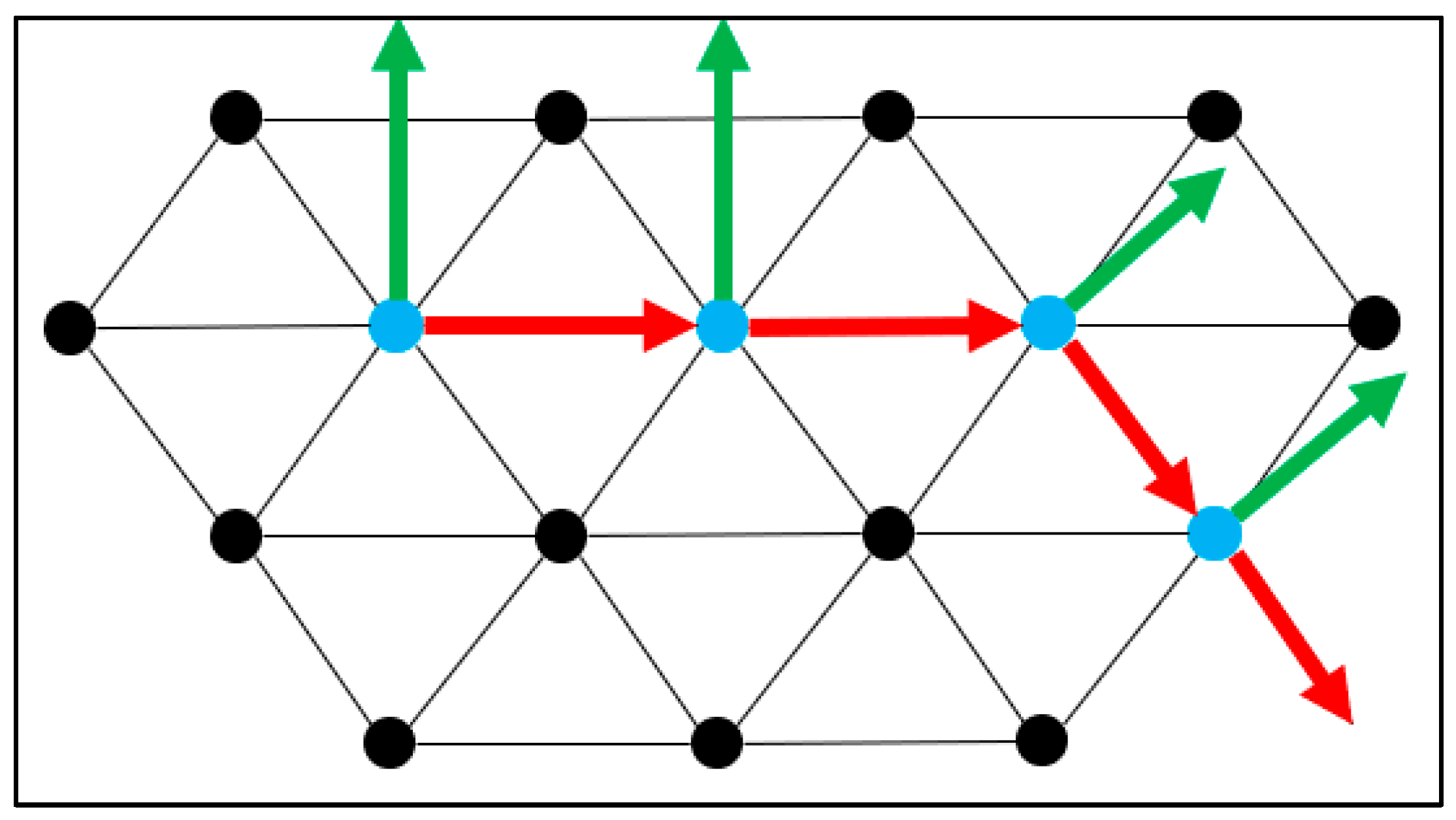
As illustrated by Figure 5, the mesh is formed by a group of nodes connected by edges. The user can select the maximum and minimum edge lengths in the mesh, which determines the resolution of the mesh. The user can select a node by clicking on it and committing the selection with a button. This interaction is made possible with MATLAB’s callbacks [20], which allow MATLAB figures to respond to user input. Each time the button is pressed, it invokes a callback, which appends the ID of the selected node to the array of the selected nodes.

The nodes of the trajectory must be selected sequentially. The order of the appended nodes in the array of selected nodes is the exact same order in which the waypoints of the trajectory would be traced. The nodes in the array of the selected nodes can be repeated.

The array of the selected nodes and the mesh are used as inputs for an algorithm for path planning in the surfaces of a mesh, developed with the functions of the MATLAB PDE Toolbox [18]. Once the path over the surface of the mesh is traced, both the path and the mesh are used to calculate the pose of each waypoint of the trajectory. Both the path planning algorithm and the pose calculation will be explained in further detail in Section 2.4.1 and Section 2.4.2, respectively.

It is worth highlighting that, during the selection of the nodes for the trajectory, the trajectory traced by the selected nodes is shown to the user. Depending on user selection, the interface can show the nodes of the trajectory as markers or as poses on the surface of the mesh. Figure 6 illustrates the difference: both meshes and trajectories are the same, but each one has a different representation for the nodes. The trajectory in Figure 6 has, in total, 76 nodes, where only 3 are the nodes selected by the user. The other 73 nodes were used by the path planning algorithm to connect the 3 nodes selected by the user; the path planning algorithm is explained in further detail in Section 2.4.1.

2.4. From Surface Nodes to Pose Trajectory

Considering that the user has selected the correct set of points on the mesh, the next process is to transform those nodes into a pose trajectory that the robot can understand. To achieve such transformation, the following next steps are required:

• Path Planning over a mesh Surface
  • Nearest Node from List;
  • Nearest Node from Face;
  • Middle Surface Node;
  • Surface Path.
• From Surface Path to pose Trajectory

All those steps are extensively described in the following subsections.

2.4.1. Path Planning over a Mesh Surface

In order to give a more comprehensive explanation of the path planning algorithm, it is divided into 4 smaller and simpler algorithms. The result is 4 algorithms that together make path planning possible; each algorithm builds in both the previous algorithms and the PDE Toolbox [19]. The following list gives the denomination given to the algorithms and the purpose:

(1)

Nearest Node from List: Given a list of nodes and a spatial point, return the node on the list nearest to the spatial point;

(2)

Nearest Node from Face: Given a face of the DGM and a spatial point, return the node in the face nearest to the spatial point;

(3)

Middle Surface Node: Given two nodes in the surface of the mesh, it calculates the spatial midpoint between the two nodes, and it returns the surface node nearest to the spatial midpoint;

(4)

Surface Path: Given a sequence of nodes, it returns a sequence of surface nodes, which connects the nodes of the original sequence.

Before the explanation of the algorithms, it must be clarified that the classes DGM and mesh and their respective attributes and methods are used in this section. For further information, it is recommended to read the documentation of the PDE Toolbox [19]. There are attributes and methods of the classes of the PDE Toolbox [19] that are referenced in the figures of the following subsections. The attributes are placed inside a red regular rhomboid and are denominated as “geometric information”. The methods “findNodes” and “nearestFace” are depicted as predefined processes in the flowcharts inside orange rectangles with vertical parallel lines.

Nearest Node from List

The first algorithm is the “Nearest Node from List” illustrated in Figure 7. The algorithm receives a list of IDs of nodes and the coordinates of a spatial point. The distance vectors between the spatial point and each node in the list are calculated. The magnitude of each distance vector is calculated as well. Both the smallest magnitude of the distance vectors and the ID of the node used to calculate the smallest distance vector are returned as the result.

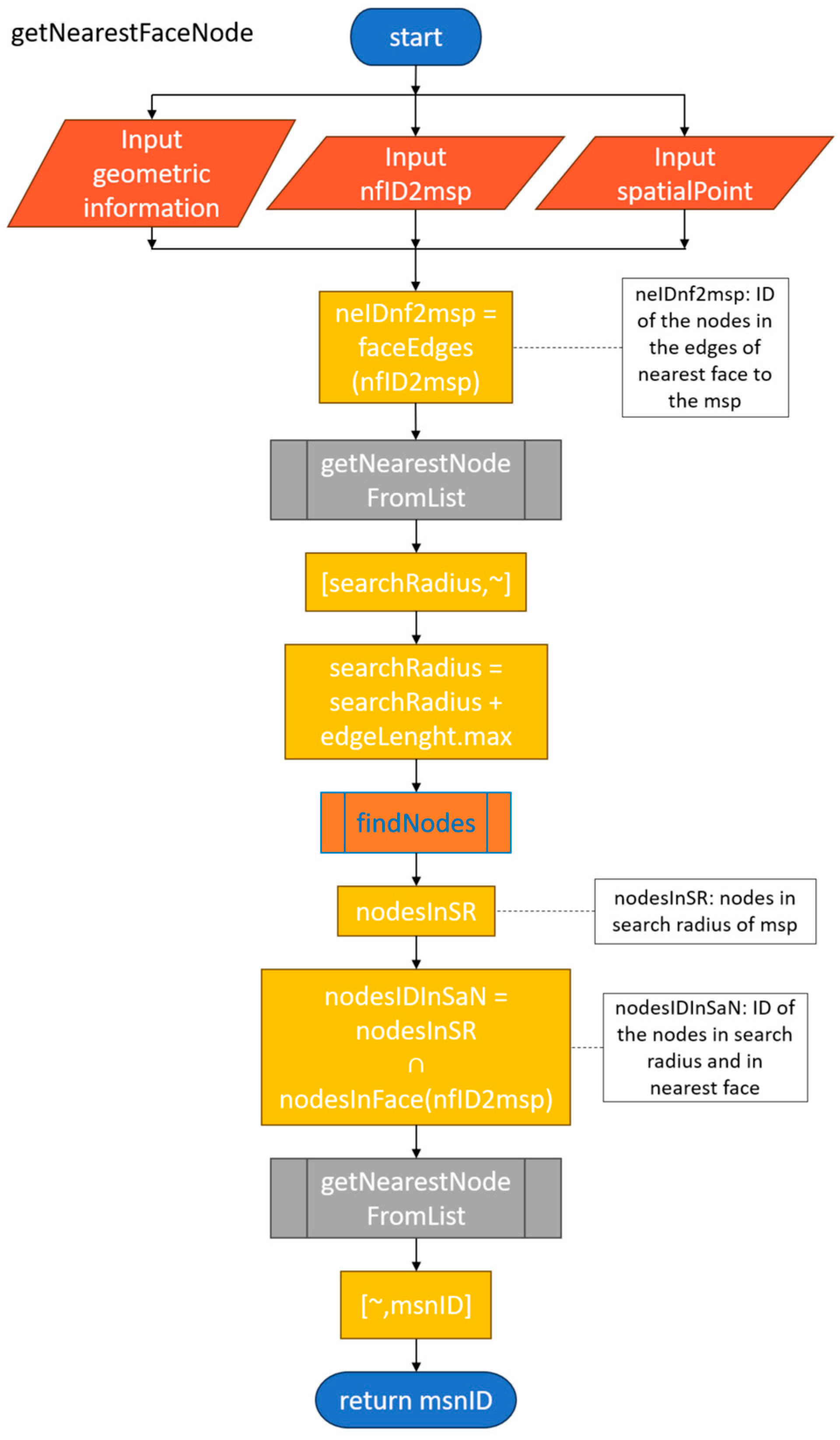
Nearest Node from Face

The second algorithm, the “Nearest Node from Face”, is illustrated in Figure 8. The inputs of the algorithm are the coordinates of the spatial point and the ID of the nearest face to the spatial point. Using the ID of the nearest face and the attributes of the DGM, the nodes on the edges of the nearest face to the spatial point are extracted. The nearest face ID and the spatial point are input to the Nearest Node from List to achieve the shortest distance between the spatial point and the edges of the nearest face.

The shortest distance plus the maximum edge length of the mesh becomes the radius for the search volume centered in the spatial point. The method “findNodes” uses the spatial point and the search radius to return a list of the IDs of the nodes inside the search radius. Using the ID of the nearest face and the attributes of the DGM, the nodes on the nearest face to the spatial point are extracted.

A node array is created with the intersection of the array of nodes in the nearest face and the nodes inside the search radius. It is worth noting that the search radius is calculated with the distance of the nearest node in an edge of the nearest face plus the maximum edge length. By calculating the search radius with the nearest edge node, it is guaranteed that the intersection of the arrays has at least one element.

Using the intersection array and the spatial point as inputs to the Nearest Node from List to achieve the ID of the nearest node in face, without the need to search all the nodes in the face.

Middle Surface Node

The third algorithm, the “Middle Surface Node”, illustrated in Figure 9 uses two nodes to calculate the coordinates of the spatial midpoint (msp). The msp is used with both the DGM method “nearestFace” and the mesh method “findNodes”, to find the nearest face and the nearest node, respectively.

If the nearest node is in the nearest face, the Middle Surface Node ID (msnID) is found and the algorithm ends. If the nearest node is not in the nearest face, the Nearest Node from Face algorithm must be used to obtain the msnID.

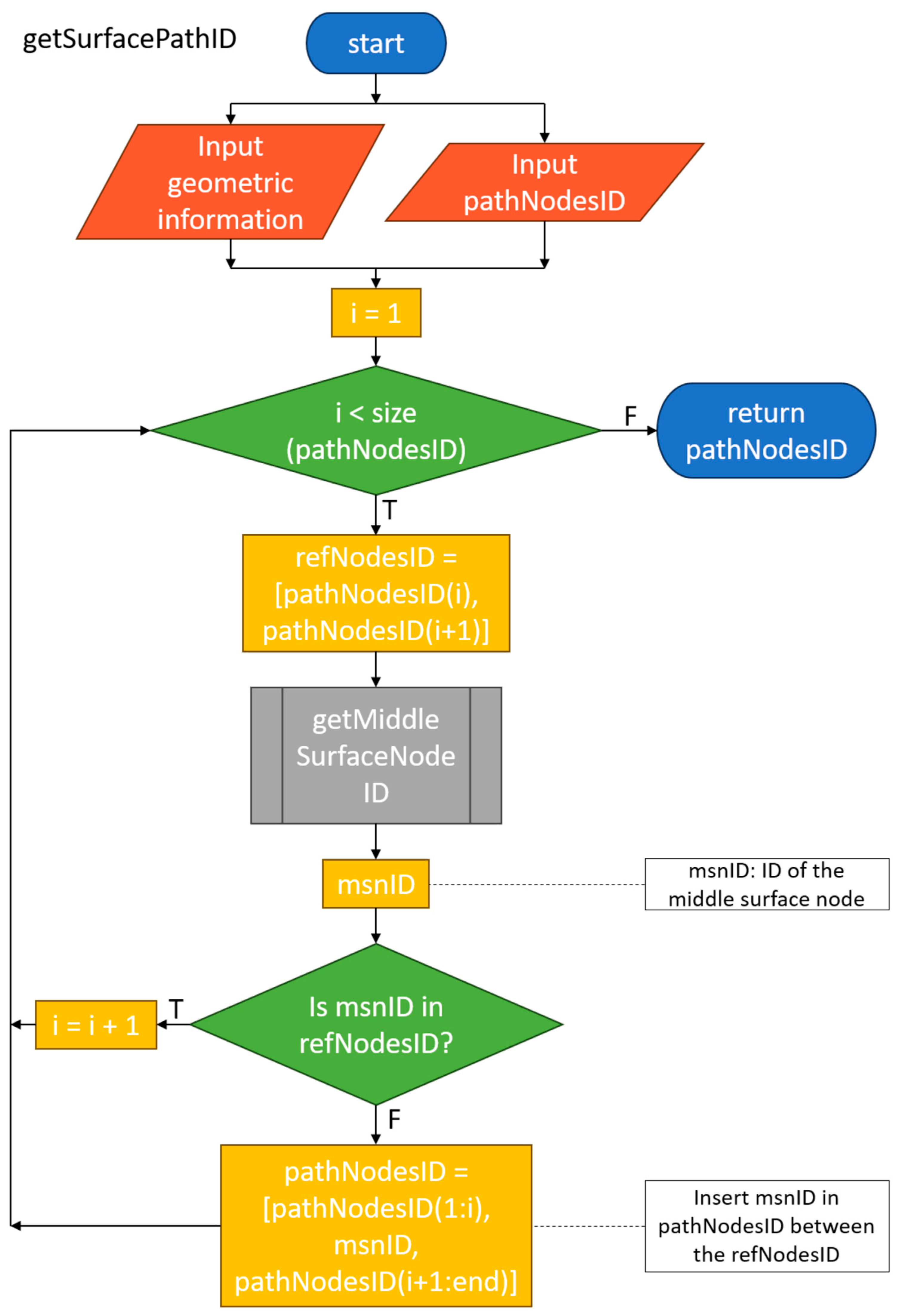
Surface Path

The fourth algorithm, the “Surface Path”, illustrated in Figure 10, takes the array of user-selected nodes as input. It initializes a counter, denoted by the letter i, and iterates through pairs of nodes in the array until the counter is equal to or greater than the size of the array. The node pairs are the nodes in the place i and i + 1. In an iteration, it uses the current node pair, referred to as reference nodes (refNodesID), as input for Middle Surface Node to obtain the Middle Surface Node ID (msnID).

If the msnID is one of the refNodesID, it is implied that there is no intermediate node between the refNodesID. The refNodesID are connected, the counter is incremented, and a new iteration starts.

If the msnID is not one of the refNodesID, it is implied that the new node is an intermediate node between the refNodesID. The new node is inserted in the array between the refNodesID in the i + 1 position, and a new iteration starts.

Once the counter is equal to or greater than the size of the array of user-selected nodes, the algorithm outputs the resulting array of user-selected nodes connected by surface nodes.

2.4.2. From Surface Path to Pose Trajectory

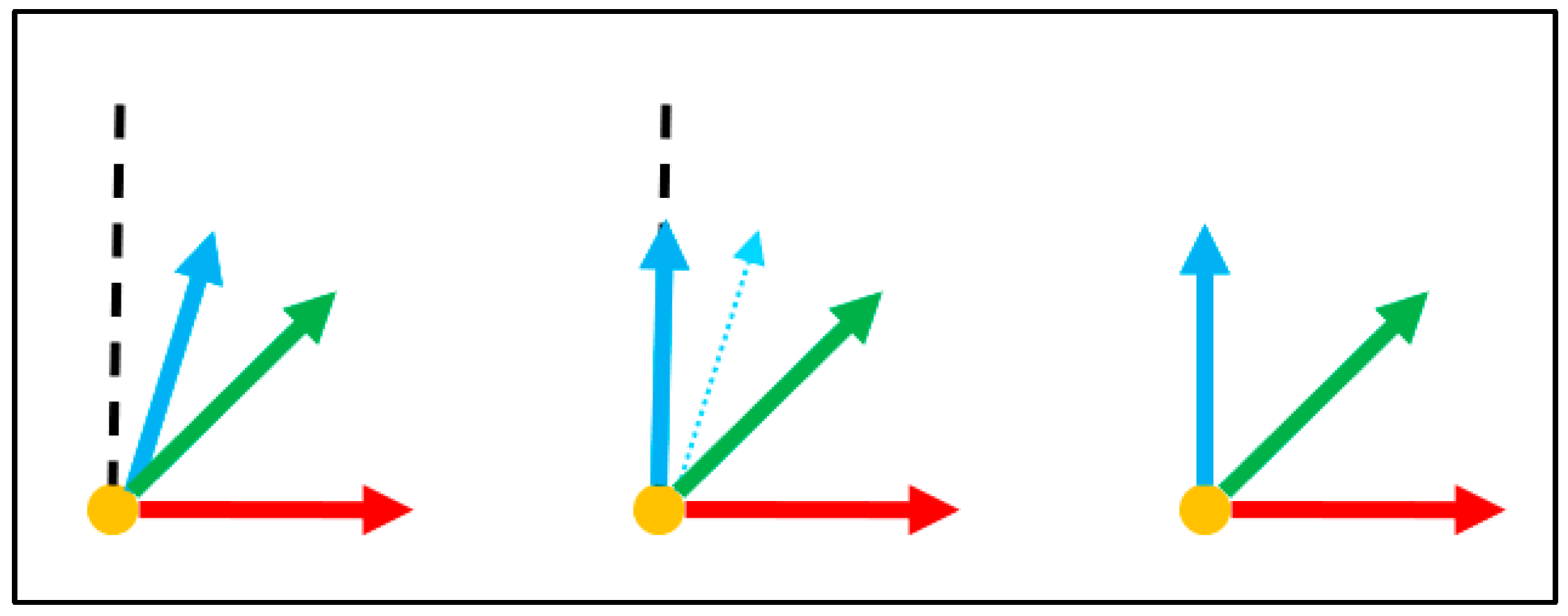
Once the surface nodes have been linked together by intermediary nodes, the position that the TCP of the cobot must take to get to each node is available. However, the orientation of the TCP is still unknown. In order to calculate the orientation components of each pose, for each waypoint of the trajectory, three-unit vectors must be calculated.

The X and Y components of the orientation parameter are straightforward to obtain. However, the Z unit vector must be calculated three times before it provides enough verifiable information.

The first calculation of the Z unit vector, as can be seen in Figure 11, is used to distinguish between the interior and the exterior of the model.

The second calculation of the Z component, shown in Figure 12, gives, as a result, the normal vertex of Z from the normal vector of the surface plane. This unit vector closely reassembles an ideal normal unit vector to describe the differential plane, but it is not used as the final unit Z vector for two reasons. First, depending on the features of the surface, the unit vector could deviate from the desired normal unit vector; this is caused by the method to calculate the normal vertex. Second, the method does not ensure orthogonality with the other two unit vectors of the pose; orthogonality is addressed later in this process.

Afterwards, the vector components X and Y are calculated separately. The X component of the pose, as shown in Figure 13, is obtained by calculating the displacement vector between consecutive reference nodes; the unit vector of the displacement vector is the X component of the pose.

The Y unit vector is calculated by performing the cross product vector operation between the Z and X unit vectors in that order, as pictured in Figure 14.

To ensure orthogonality between the X and Z unitary vectors, which is required for a pose, the Z component is calculated a third and last time using the cross product of X and Y unit vectors. As the cross product vector operation renders a third vector perpendicular to both X and Y unit vectors, this last calculation is used to secure orthogonality among the three calculated components. This adjustment is illustrated in Figure 15.

These five steps, the three calculations of the Z component and the X and Y component calculations, are repeated for each waypoint in the trajectory. The resulting poses are saved in a pose array; the poses are saved in the same sequence as the resulting waypoint array from Section 2.4.1. The pose array is used for simulation, explained in Section 2.6.

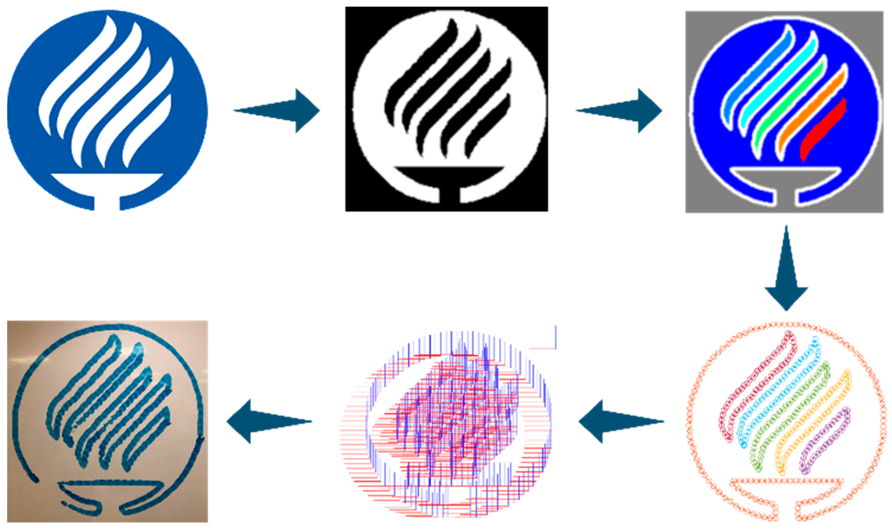
2.5. Image-to-Trajectory Conversion Algorithm

For 2D trajectories, the complexity of the trace can be incremented since the additional configurations used to adjust the cobot to the 3D surface are not necessary. Instead of letting the user choose the individual points in the trajectory, 2D traces were acquired by analyzing provided JPG images and identifying their edges with an image processing algorithm called the Otsu Method [21]. Then, the contour of the objects in the image is mapped to trajectory poses, which can then be converted to a script executable by the robot.

The first step to generate a trajectory in a 2D surface is to upload a JPG image. Using the MATLAB Image Processing Toolbox [22], the original image is converted to black and white for ease of processing. The result is then rotated 180 degrees in order to facilitate the conversion from image space to 3D spatial coordinate space. The process is graphically represented in Figure 16.

After the rotation, the image is binarized in order to prepare it for an adequate performance in the execution of the edge detection algorithm. The contour of the objects represented in the image is identified using the MATLAB Image Processing Toolbox [22]. Once the edges have been detected, a series of trajectory poses can be obtained from them. In Figure 17, the results of the binarization and edge detection processes are shown. For ease of visualization, the previous 180° rotation was omitted.

After the contours of the objects are obtained, minor adjustments are made to improve the performance of the robot while tracing the trajectory. These adjustments include removing small imperfections in the image that may be perceived as objects and, for performance reasons, the extraction of only a fraction of the points of the trajectory. With these adjustments, the transformation from the image coordinate system to the spatial coordinate system is as follows in

Table 1. Image coordinate system to spatial coordinate system transformation.

Image Coordinate System	Spatial Coordinate System
Y coordinates	X coordinates
Defined by user	Y Coordinates
X coordinates	Z Coordinates

.

Once the trajectory is expressed in poses, it is expanded or contracted in order to fit the designated drawing space. In Figure 18, the image was adjusted to fit in a 200 mm by 200 mm square.

Once the trajectory has been successfully adapted to the drawing space, it can be saved and exported for simulation, which is further explained in Section 2.6.

2.6. Trajectory Simulation

To simulate the trajectory that was generated in the previous step, a digital representation of both the robot and the surface must be created.

Using the MATLAB Robotics Toolbox [23], the Robot model of the UR5 is imported. This model is used to set up the Inverse Kinematics Solver (IKS), which will render the configuration of the robot for the desired TCP poses. Afterwards, depending on the application, a trajectory from a CAD model or from an image is imported into the script. Once the trajectory is imported, the user must select some parameters for the simulation, such as the speed at which the TCP will move and the setup adjustments for the TCP pose with respect to the trajectory pose.

After the setup of the trajectory initial parameters, the IKS solves for the configuration of the robot in each pose of the trajectory, executing a linear movement.

The trajectory is graphed prior to the simulation. Then, the robot model and (if needed) the CAD model are placed in a 3D space for the simulation. Information such as the type of movement, the TCP pose, and the robot configuration is saved for the program generator algorithm.

Finally, after obtaining all the poses and configuration spaces that conform to the trajectory, a CSV file containing this information is generated. The structure of the rows in this file follows the structure shown in

Table 2. Comma Separated Values CSV column structure.

Data	Movement Type	Pose		Configuration Space
		Position	Orientation	Joint Angles
Data Index	0	1–3	4–6	7–12

. Available movement types were encoded (MoveL = 0, MoveJ = 1, etc.), position and orientation components of the pose were saved, and, finally, joint angles were added when relevant to the movement type.

2.7. Parsing from CSV to URScript^®

URScript^® is a proprietary scripting language from UR [16]. Polyscope is the proprietary Integrated Development Environment (IDE) for programming the UR robots with URScript^® [16]. More detailed information can be found in the URScript^® Programming Language Manual [16].

The process of generating URScript^® code using the information contained in a CSV file was achieved using Python and will be referred to as parsing in the different steps of development described in this paper.

For starters, the configuration space and pose classes were created for the abstraction of these concepts; more information about their content can be found in Figure 19 and Figure 20, respectively.

The process followed is graphically represented in Figure 21. The previously mentioned CSV is read and for each row, according to the movement type, information regarding poses or the cobot’s configuration space is stored as different instantiations of these classes. Then, with the use of an overridden __str__ method, this information is converted into string and used to generate the corresponding movement functions (MoveL, MoveJ) that will set the TCP position and orientation changes with a specific characteristic such as blend radius or desired configuration space, the corresponding equivalent command that the robot OS will read and interpret.

These commands are concatenated and, in the end, a .script file that contains all the waypoints needed to recreate the desired trajectory is created.

The selection of the CSV file and the destination of the generated .script file is obtained via a Graphical User Interface developed using the Tkinter library, as can be seen in Figure 22.

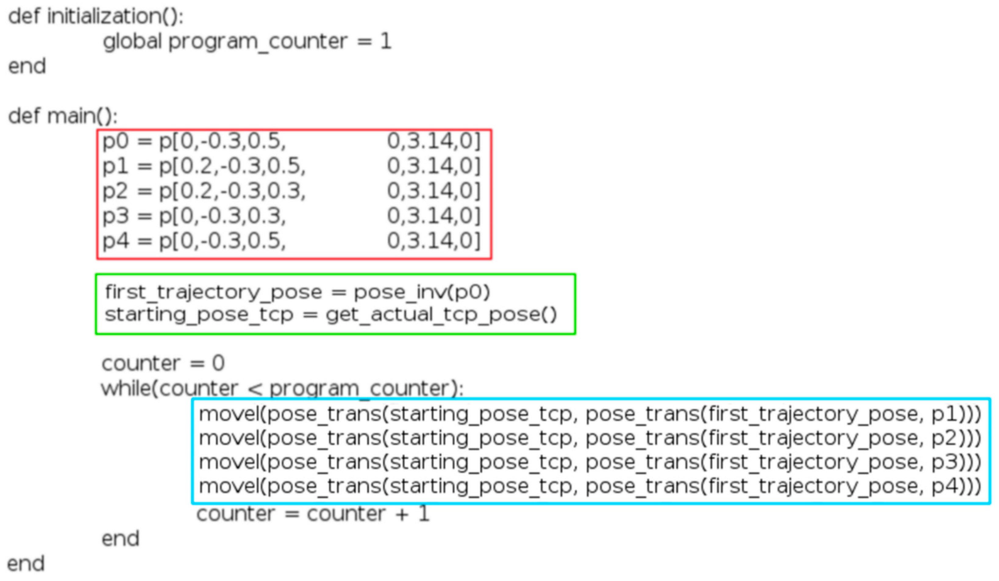
The resulting .script file contains two functions that are run in a .urp file: an initialization and a main.

The initialization is used to set up variables that can manipulate the program flow. An example of this manipulation is the variation in the number of times the user wants the trajectory to be followed by the TCP.

The main includes all the information regarding the movements, poses, and desired configuration spaces that conform to the trajectory. It is important to add that all these movements and poses are made relative to the starting pose of the TCP.

Figure 23 illustrates an example of an output file. The red rectangle contains waypoints in the absolute frame of reference; the green rectangle contains the necessary transformation to take the waypoints to a relative frame of reference, and the blue rectangle contains the movements between waypoints in this new frame of reference.

3. Results

It must be reiterated that the project is proof of concept; its primary objective is to assess the feasibility of the proposal, and for that reason, the test and its corresponding results are qualitative. The tests were divided between the 2D and 3D trajectories.

The 2D case studies were primarily used to validate the work achieved in Section 2.6 and Section 2.7 and to evaluate the performance of the robot executing the trajectories. It is worth noting that the 2D scripts were also used in a demonstration for the general public, special guests of the university in which the project was developed, recruitment events, and science fairs.

The 3D case study was used to test the main application of the project. First, it was necessary to validate Section 2.3 and Section 2.4. Once Section 2.3 and Section 2.4 were validated, the next step was to integrate them with Section 2.6 and Section 2.7.

3.1. 2D Case Studies

3.1.1. Lightning

After creating the simulation in MATLAB and the parser with Python, coordinates of simple 2D shapes were manually typed and converted into CSV files to test the integration between the modules developed in Section 2.6 and Section 2.7. In Figure 24, from left to right are the main points generated manually for the test, the path generated to connect the main points, the pose trajectory for the TCP of the robot and the drawing made by the robot using the main points.

3.1.2. Logo

The image processing algorithm based on the Otsu Method module described in Section 2.5 was introduced to test the behavior and integration of the modules of Section 2.6 and Section 2.7 with more complex shapes. Although it is true that more advanced image processing algorithms exist, it was outside the scope of this research, and for that reason, a comparably simpler algorithm was used.

The images for the test had to be digital drawings with high contrast between the foreground and the background, although sometimes constraining the algorithm was good enough for our purposes. In Figure 25, the emblem of our university was used for the first test of the image processing module. The robot was able to draw free hands on a plain surface. It is worth highlighting that the system can draw circles and other curved lines.

The objective of this test was to validate the integration of the module of Section 2.5. For such a reason, the resolution of the path was minimized to make a meaningful reduction in the strain endured by the cobot, but high enough to still have a well-defined shape. This drawing has 455 waypoints.

Although it is outside the scope, it is worth highlighting that the Section 2.5 module was later repurposed for demonstration, and it was used in poster exposition, career fairs, and company visits, among others. The modification, which at that moment was an afterthought, had a huge positive impact on the project. The project was well received, it attracted a lot of attention, and it generated interest, which in turn opened many doors that ultimately helped to continue its development.

The attendees of the demonstration, which included the general public, colleagues, students, faculty members, companies, and special guests, were engaged with the project and were amazed by the result. The success of the project was influenced by the support of the public: the seemingly trivial change to the system allowed a lot of different people, including people without technical or engineering backgrounds, to connect with STEM.

3.1.3. Tecnológico de Monterrey

Once it was validated that the module of Section 2.5 worked with a complex image, the system was tested to observe its performance with a trajectory that contained a much bigger number of waypoints. The process shown in Figure 25 was done with a more complex image to evaluate the capabilities of the module. For this test, the emblem and the name of the university were used, and the result is shown in Figure 26. The drawing has 1606 waypoints.

Further tests were made to try to increase the resolution of the drawings, but it negatively affected the performance of the cobot. It was not possible to pinpoint the maximum quantity of points allowed in a drawing, but from the conducted tests, it was possible to determine that the robot demonstrated a good performance if the maximum number of points stayed in the range from 1800 to 2400 waypoints. The physical aspect of the robot itself was the main limiting factor on the maximum quantity of waypoints in the trajectories. Although it is possible to make the robot execute such trajectories, it is recommended to keep the quantity of waypoints inside the aforementioned range.

3.2. 3D Case Study

Before tracing a 3D trajectory, the modules in Section 2.3 and Section 2.4 were validated individually.

The module of Section 2.3 was validated with a functional test. The module was modified in order to plot the user-selected nodes during selection. This helped the tester identify which nodes would be appended and which nodes had already been appended. After each test, the list of nodes was verified manually.

The module of Section 2.4 was split into two parts for its validation, namely Section 2.4.1 and Section 2.4.2. The submodule of Section 2.4.1 was modified to plot the array of nodes generated by the code. Once the tester saw that the selected nodes had been connected automatically, the module was validated. The submodule of Section 2.4.2 was validated with almost the same method as the previous submodule. The only difference in the latter’s validation was a closer inspection from the tester, making sure the orientation of the poses was congruent with the desired outcome. The direction of the unit X vector had to have the same direction as the trajectory, the unit Z vector had to be perpendicular to the surface, and all three unit vectors had to be perpendicular to each other.

Tumbler

After validating all the required modules for 3D trajectories developed in Section 2.3, Section 2.4, Section 2.5, Section 2.6 and Section 2.7, a test on a physical 3D surface was conducted.

Insofar as 3D surfaces are concerned, only regular geometric shapes were considered. The robot was able to trace a trajectory on a cylindric surface. The trajectory can be observed in Figure 27. The uncertain traces are caused by the resolution of the mesh, which could not be smaller than 7 mm due to hardware limitations.

4. Discussion

The paper presents a procedure to implement a low-cost CAM trajectory generator. This first implementation allowed the users to develop trajectories for a robot on regular 2D and 3D surfaces. As this is the first approach, it meets the expectations initially stated as the scope of the project, but there is room for many improvements that must be made to enhance the performance of the trajectory generation system.

As detailed in Section 3, the trajectories over 2D surfaces present the most satisfactory results. The algorithm was observed to process the waypoints quantitatively better than in the 3D surface test since 2D surfaces require fewer calculations for the conversion of the points into a URScript^® program. Even though these results were satisfactory, they can be improved by optimizing the number of waypoints required. In that way, the trajectory can be generated successfully by using interpolation to obtain a lower resolution if needed.

In the case of the 3D trajectories, the results using the mesh to select the trajectory rendered satisfactory results within the scope of the initial expectations set by the scope of this project. However, there is room for serious improvements, such as the resolution of the mesh and the user interface to select the path on the mesh. Those are key elements to optimize the existing processes and should be addressed in order to provide a better resolution on the trajectory provided the robot is implemented.

At this moment, the solution is implemented on different software programs, starting with MATLAB and then using the parser to generate the trajectories. This integration accomplishes the goal of implementing the trajectory and getting the robot to follow the path, but using many platforms could be confusing for the final user, so it would be useful to integrate the whole solution on a single platform. Many ideas can be used, but to maintain the objective of the project to be a low-cost application and an open-source solution, the selection must be made carefully. For example, instead of using MATLAB for the generation of the waypoints, it could be substituted using ROS as the simulation environment to obtain the points required for the application.

The integration with ROS is a suitable solution that can benefit the development of the platform since it could help in simulating the complete environment in which the robot will be working. If the whole environment is on the simulation model, there could be an opportunity to develop a collision avoidance system to improve and optimize the path planning of the robot.

In conclusion, the system presented in this paper is the first approach to create an open-source solution for path planning for robot applications, such as welding or gluing. It could be used as the base of an open-source software for industrial applications. The improvements can be added over time, and the opportunity to develop better methods will create a community for the maintenance and improvement of the platform.