Article

Unveiling Inertia Constants by Exploring Mass Distribution in Wind Turbine Blades and Review of the Drive Train Parameters

by
Angel Gaspar Gonzalez-Rodriguez
1,*,
Juan Manuel Roldan-Fernandez
2,† and
Luis Miguel Nieto-Nieto
1,†
1
Department of Electronic Engineering and Automation, University of Jaen, 23009 Jaen, Spain
2
Department of Electrical Engineering, Escuela Técnica Superior de Ingeniería, Universidad de Sevilla, 41092 Sevilla, Spain
*
Author to whom correspondence should be addressed.
These authors contributed equally to this work.
Machines 2023, 11(9), 908; https://doi.org/10.3390/machines11090908
Submission received: 7 August 2023 / Revised: 8 September 2023 / Accepted: 11 September 2023 / Published: 13 September 2023
(This article belongs to the Special Issue Estimation and Mitigation of Fatigue Damage for Wind Turbines)

Abstract

:
In studies of dynamic stability and power quality, it is necessary to know the values of the mechanical parameters determining the transient response of wind turbines. Their exact values are not as decisive as the power curve, but an inaccurate estimate can distort or even invalidate the simulation results. From a review of the literature, it has been found that, despite their importance, the values of inertia, stiffness and damping are hardly available for any turbine model. Another detected problem is the lack of confidence in the data origin. This article aims to solve the issue of the scarcity and unreliability of data on inertia, and gathers the information found on the remaining mechanical parameters. Available blade inertia values in kg · m 2 are presented. Special treatment has been given to those providing the mass distribution along the blade span, for which the provided values of inertia have been compared with those obtained numerically, showing good matching. With this, different reliable relations are obtained that allow for the calculation of the turbine rotor inertia, based on the mass and length of the blade. When the center of gravity is also available, a very correlated expression ( r 2 = 0.975 ) is provided to obtain the inertia. The references to the stiffness and damping constant of the drive train, which are even more rare, will also be presented. In addition, the study includes a revision of gearboxes, generators and blade weight, according to their IEC-class and material.

1. Introduction

1.1. Context and Purpose of the Work

In power system stability studies, it is important to have an appropriate model for the characterization of a physical phenomenon of interest. Depending on the analysis to be carried out, the corresponding models may be different. According to the time scale of interest for stability studies, the models can be classified as electromagnetic models (to scale short time frames) or electromechanical models to investigate slower events. The influence that modeling can have on the results of the study can be seen in [1].
With regard to the electromechanical models, the most important components to take into account are the turbine inertia, the generator inertia and the coupling between both moving masses. In general, the inertia in AC electrical power systems represents the kinetic energy stored in large rotating generators and synchronous motors, providing them with the tendency to maintain continuous rotation. In the case of additional rotating masses (steam turbine in the case of thermal units, Francis/Kaplan/Pelton turbine in the case of hydro units or blades in the case of wind turbines), the corresponding inertia must be added to the generator value.
A system that possesses a sufficient natural rotational inertia is able to maintain the grid frequency in its rated values, since this frequency is really an electromechanical variable that is linked to the mechanical speed of rotation of the generators. When a sudden power imbalance between generation and demand occurs in the grid, a frequency deviation typically appears. If the contingency is not serious, this stored kinetic energy allows for a rapid response, permitting a transfer of energy to balance generation and load, before the frequency deviation exceeds permitted values. On the other hand, in normal operation, small variations are permitted in the electrical frequency in real time, to ensure an adequate balance of active generation and load. In both cases, abrupt or slow power imbalance, inertia plays a determining role during the balancing transient.
This kinetic energy is:
E k = 1 2 J Ω G 2
where J is the system inertia and Ω G is the rotational speed of the electrical generator [2]. It allows us to define the inertia time constant H of a generator as the ratio between the stored kinetic energy E k and its rated power. It determines the time interval during which an electrical generator can supply its rated power, by using solely the kinetic energy stored in its rotating masses [2].
Additionally, the current paradigm shift, with the incorporation of wind power and photovoltaics into the power system, is achieved using power-electronic converters that do not possess natural rotational inertia, unlike a synchronous generator (SG). Consequently, renewable generators displace synchronous generation and reduce the amount of rotating mass in the system. Therefore, system operators need to model these electrical systems with low rotational inertia, which presents significant challenges to controlling the stability of the system [3,4].
The availability of precise inertia data permits the system operator to make appropriate decisions and facilitates the improved planning and operation of the system. This ensures the stability and resilience of the network and enables the efficient integration of larger amounts of renewable generators, without compromising system security or power quality.

1.2. Literature Review

The importance of inertia in stability studies is addressed by many authors. Ekanayake in [5] shows how, with the correct control of the power electronics connected to the rotor of a doubly fed induction generator (DFIG), inertia allows the recovery of a significant amount of kinetic energy. This alleviates the effect of a frequency drop in the network system.
In the case of fixed speed induction generators (squirrel-cage type), the recovered kinetic energy is much lower since the range of operating rotation speeds is reduced to +1÷3% above the synchronous speed. At the other extreme, SGs allow a much wider speed range, and there is a decoupling between the mechanical part and the transient phenomena that occur on the network side [6], due to the IGBT-converters. Initially, this decoupling could lead to a reduction in inertia seen by the network, and therefore, less damping against abrupt changes in generation and charging patterns [7,8]. This has given rise to a multitude of articles on frequency control strategies to effectively integrate wind energy systems into the grid. In any case, for the evaluation of the kinetic storage capacity, it is necessary to know, as precisely as possible, the inertia value for the turbine and the generator. It is also mandatory to be familiar with the mechanism for the transmission of kinetic energy between both components through the coupling, for which it is necessary to have an understanding of its characteristics of stiffness and damping.
Guillamon in [9] performs a review of inertia data, and although providing its dimensionless value, it is difficult for some references to trace those which have been reliably obtained. Other authors such as Morren in [6] assume, in the absence of reliable data, that the geometry of the blade is very complicated, and approximate this to a bar of constant chord and constant, with which they obtain a simple expression to calculate inertia as a function of power.

1.3. Research Gap and Motivation

Despite their importance in system stability and power quality studies, these parameters, especially that of inertia, but also the stiffness and damping constant of the drive train, are rarely available for the turbine model under investigation. Therefore, the researcher must often carry out a study on which parameters to use in order to faithfully reproduce the actual situation. The alternative is to rely on the value used by other researchers, without any assurances that these can be adapted to the characteristics of power, length or weight of their own system.
As a result, it is highly desirable that future studies on stability and, in general, on the dynamic behavior of wind turbines contain reliable data, so that the modeling of the system is as realistic as possible. These parameters logically depend on the size of the turbine. Even using a dimensionless formulation, which converts the magnitudes into per unit (p.u.), these parameters have a certain dependence on power and, as power grows over the years, it is necessary to update the available databases with the values that can be extracted from modern machines.

1.4. Contribution

In this article, in addition to reviewing realistic data on inertia, mainly from multi-megawatt turbines, it is intended to trace the references that provide data on the density distribution (DD) of real blades, preferentially with designs based on realistic dynamic and structural analyses. From these, the calculation of the inertia of the blade will be made, and a relationship with some specific magnitude of the geometry will be deduced, such as the position of the center of gravity (CoG).
This method of obtaining inertia is novel, and is intended to be the initial stage of a more extensive database to provide reliable data on inertia, unlike inertia data obtained by transient analysis or other non-direct methods.
Although minor, other components also influence the dynamics of the mechanical system, the precision of which will depend on the number of masses with which the mechanical part of the turbine is modeled [10,11]: generator inertia, hub inertia and stiffness/damping of the power transmission shafts between the turbine and generator. The relationship between the different mechanical variables will be reviewed through these parameters, and the corresponding expressions converted into dimensionless values. In [11], it is stated that it is possible to reduce the number of masses of the drive train model, without significant deviations.
The theoretical and technical contributions of this paper are to:
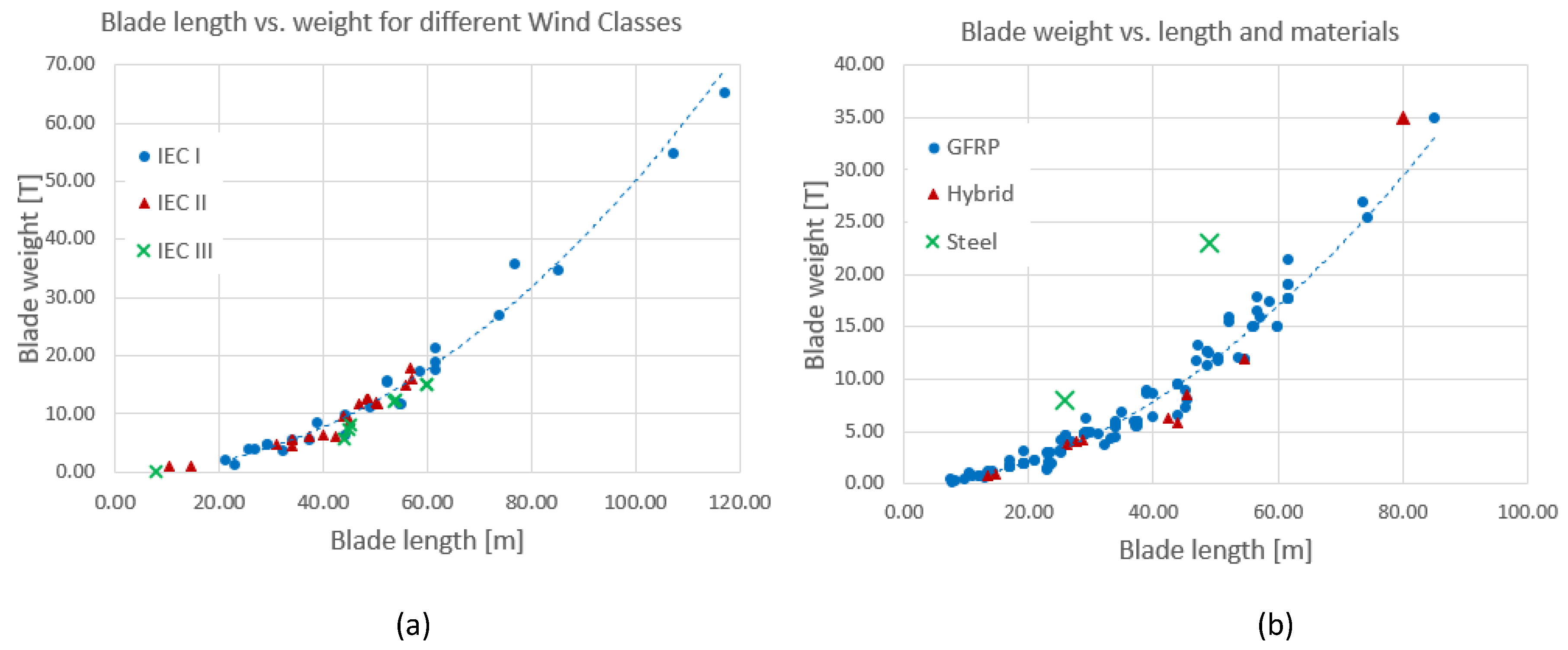
  • Provide general expressions that allow the weight of the blade to be estimated based not only on its length, but also on the IEC wind class of the turbine and the material of the blade.
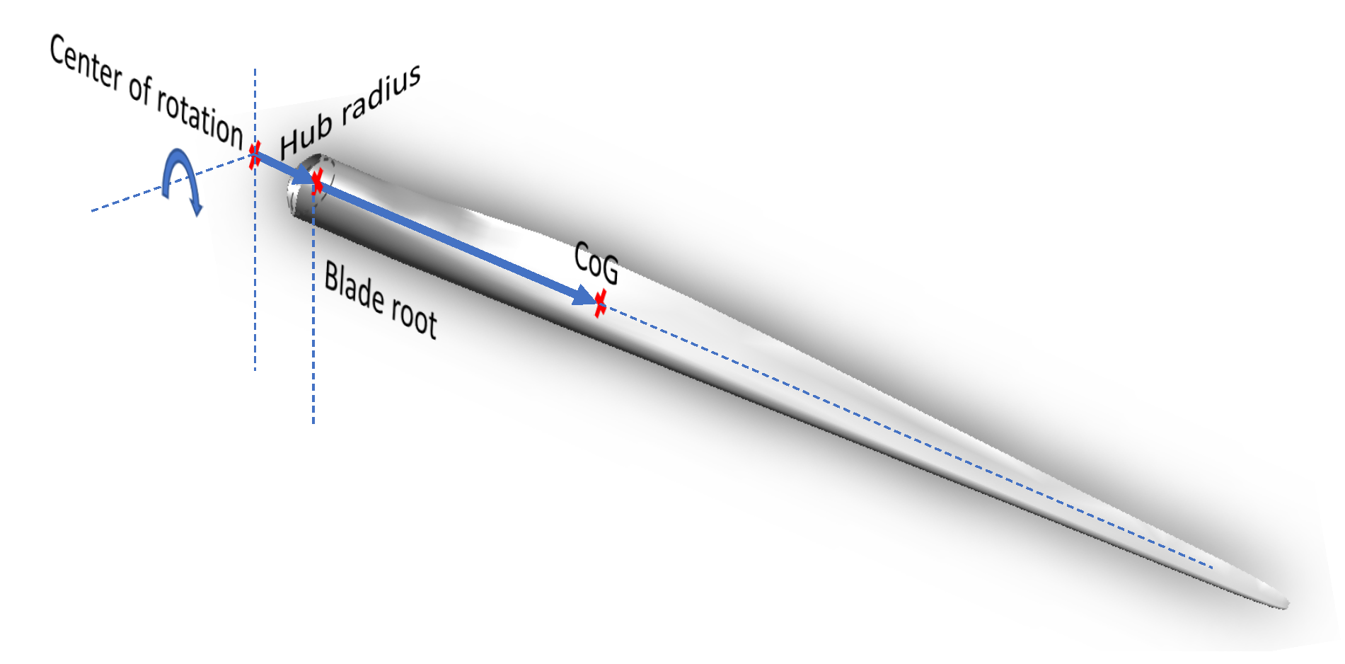
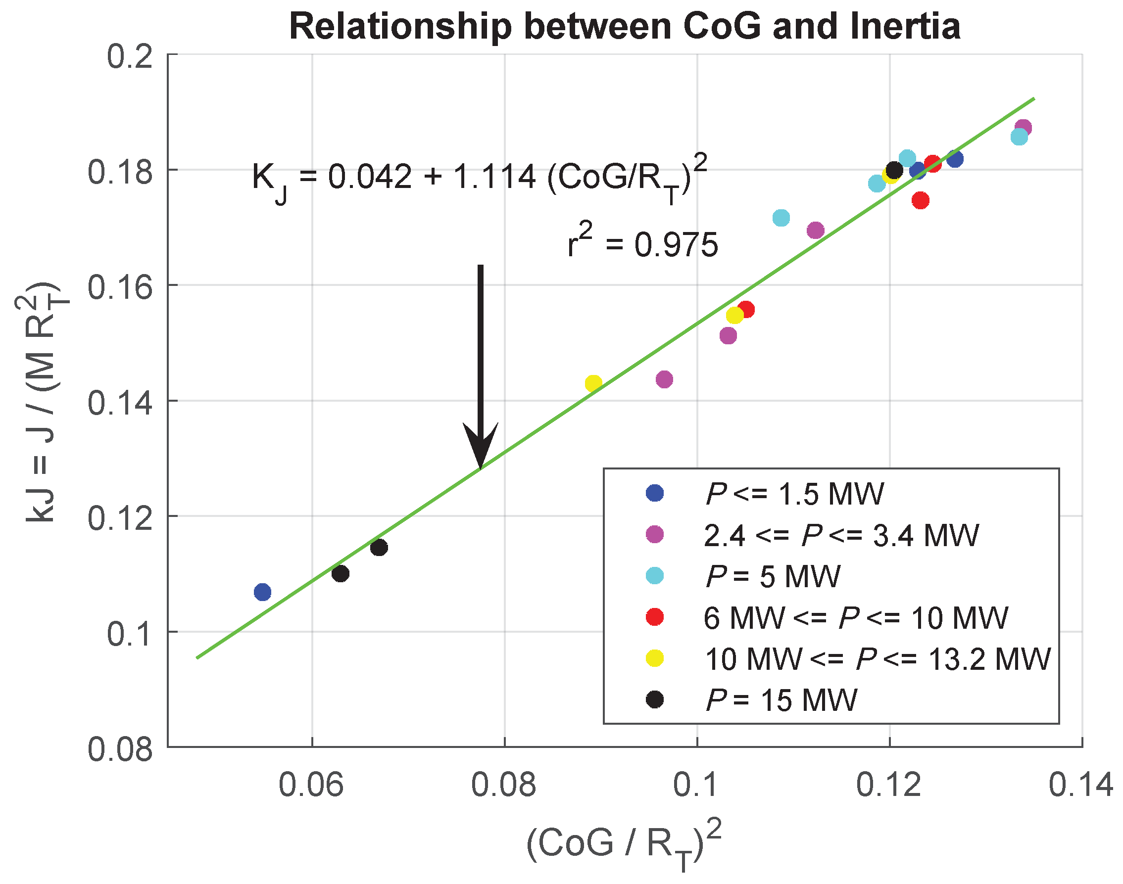
  • Provide an expression that accurately estimates the blade inertia starting from the position of the CoG, its weight and its length.
  • Formulate in depth a complete dimensionless framework to relate magnitudes and parameters (such as inertia, damping, stiffness and friction) with respect to their base references, valid for systems of three masses and two masses.

1.5. Paper Organization

The rest of the article is explained below. In Section 2, the mechanical equations that govern the rotation movement of each component are reviewed, the expressions that transform each variable and parameter into its value in p.u. are shown and certain general, distinguishing characteristics of each parameter are described. In Section 3, all the data retrieved on the DD of 21 blade models are organized, and a relationship is identified that links the inertia with the position of the CoG of the blade. The values obtained for the other parameters reviewed are also organized. Finally, in Section 4, the results are evaluated, highlighting the achievements obtained as well as their limitations.
At the end of the paper, a list of abbreviations and variables is included.

2. Methods

This section formulates the expressions governing the dynamics of the interaction between rotor and generator and how they can be converted into p.u. It also anticipates certain issues to be taken into account prior to listing the revised data.
Hereinafter, the set of blades plus hub will be named as the turbine rotor or simply turbine, and this will appear referenced in the expressions as T. A blade will be designated as B, the generator as G and the gearbox as G B . Magnitudes and parameters with dimensions will appear in uppercase, and their conversion to p.u. will be displayed in lowercase.

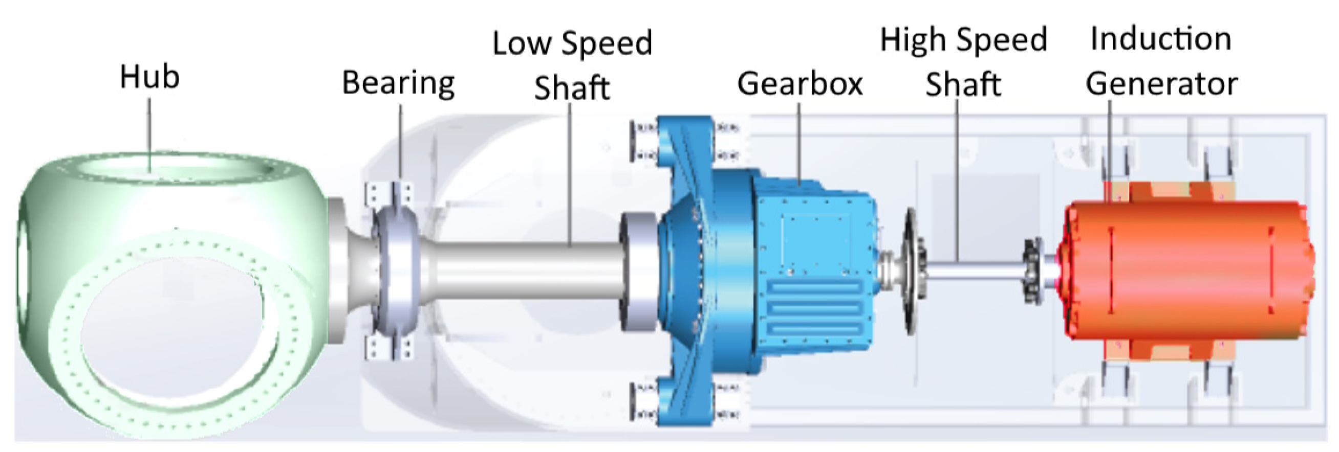
2.1. Dynamics Rotor-Generator

Once the blades extract the aerodynamic energy from the wind and transform it into a rotation torque T W exerted at the turbine speed Ω T , these magnitudes will drive the dynamics of the system until they produce a torque on generator T G , which will rotate at speed Ω G . This speed will be measured by the grid frequency, f, divided by the number of pole pairs, n p p , and will be exactly equal to this value in the case of SGs or slightly higher (due to slip) in the case of IGs in normal operation.
With regard to IGs, a high number of poles would increase the magnetization losses, so this value is reduced to no more than n p p = 2 or n p p = 3 . Since the rotational speed in rpm is equal (or very close) to 60 f / n p p with f being the grid frequency, this yields an impermissible value for blade rotation. It is, therefore, necessary to include a gearbox that accommodates both speeds. This new element introduces new equations into the dynamics of the system.
Permanent Magnet Synchronous Generators (PMSG), which are the most frequent type of SGs in wind turbines (WT), allow for a high number of poles that considerably reduce the rotational speed. In the latter case, it would not be necessary to use a gearbox. This setup is referred to as direct drive. In other schemes with PMSGs, the number of pairs of poles is not high enough to obtain the adequate speed, although in any case, the required transmission ratio decreases and with it, the dimensions and stages of the gearbox.
Other elements that form part of this transmission are the brake and the couplings that account for the misalignment between the rotation axes, although they are generally not included in the dynamic analysis of the system.
Figure 1 represents the interior of the nacelle, with the transmission chain from the turbine rotor to the generator. The scheme corresponds to an IG or a PMSG with a reduced number of poles. In this case, to accommodate the high speed in the generator shaft with the low speed of the blades, it is necessary to include a gearbox. Its ratio increases with the turbine rotor diameter and decreases with the number of poles. Figure 2 corresponds to this dynamic scheme, called three masses, where:
  • J T is the inertia of the turbine rotor due to the distribution of masses in the blades and, to a lesser extent, in the hub.
  • D T is the coefficient of friction due to the aerodynamic resistance offered by the blades.
  • K H G B is the stiffness constant in the slow axis that joins the hub and the gearbox.
  • C H G B is the damping constant of the torsional movement of the slow axis.
  • J G B is the inertia of the gearbox discs, measured from the slow shaft.
  • D G B is the coefficient of friction due to friction in the gearbox, measured from the slow shaft.
  • J G is the inertia of the rotor of the electric generator and the brake.
  • D G is the coefficient of friction due to friction in the generator and ventilation losses.
  • K G B G is the stiffness constant in the fast axis that joins the gearbox and the generator.
  • C G B G is the damping constant of the torsion motion of the fast axis.

2.2. Mechanical Equations

The equations that govern the dynamics in a system formed by the turbine rotor, the slow shaft, the gearbox, the fast shaft and the generator are those that correspond to the left side of the following expressions:
T W = T L S S + D T Ω T + J T Ω ˙ T t W = t L S S + d T ω T + 2 H T ω ˙ T
T L S S = K H G B Θ T L S S + C H G B Θ ˙ T L S S t L S S = k H G B θ T + c H G B θ ˙ T
Θ ˙ T L S S = Ω T Ω G B L S S θ ˙ T = ω T ω G B
T G B L S S = T L S S D G B L S S Ω G B L S S J G B Ω ˙ G B L S S t G B = t L S S d G B ω G B 2 H G B ω ˙ G B
Ω G B H S S = n G B Ω G B L S S
T G B L S S = n G B T H S S ( Ideal ) t G B = t H S S
T H S S = K G B G Θ G H S S + C G B G Θ ˙ G H S S t G B = k G B G θ G + c G B G θ ˙ G
Θ ˙ G H S S = Ω G B H S S Ω G θ ˙ G = ω G B ω G
T H S S = T G + D G Ω G + J G Ω ˙ G t H S S = t G + d G ω G + 2 H G ω ˙ G
where superscripts L S S and H S S stand for low-speed shaft and high-speed shaft, respectively (as an example, T L S S is the torque available in the LSS), Θ is the twist angle in the L S S or H S S and n G B is the gearbox ratio. The variables and magnitudes on the right hand side are the same expressions, although referred to their base magnitudes; they are explained in the following section.

2.3. Referring to Base Magnitudes

On many occasions, the value of a magnitude expressed in a measurement system (e.g., MKS) does not provide information on the operating range in which it is working and must be compared with its rated value. For this reason, it is customary to compare magnitudes, electrical or mechanical in our case, to their rated values, so that when working below rated conditions, the value will be between 0 and 1. This usually entails the adimensionalization of the parameters that intervene in the relationships between magnitudes. In most cases, the new magnitudes and parameters lose their dimensions and we then work in p.u. This facilitates computational manipulation, makes the variables independent of the capacity of the turbine to a certain extent or offers a better view of how close the operation is to overloading or idling. In the case of an ideal gearbox, this disappears when operating in p.u. The expressions, once transformed into p.u, are those found on the right side of (2)–(10), where uppercase has been used for values with dimension and lowercase for values in p.u.
In the following subsections, a set of dimensionless values for the different parameters of these equations (inertia, damping coefficients and friction coefficients) will be listed, and it will be easy to identify outlier values and mark them as unreliable. If the adimensionalization is not carried out, the normality range for each parameter will depend on other variables (power, speed, n G B ), so its identification is more difficult.
The relationships between variables with dimensions and in p.u. are the following:
T W = t W T B L S S with T B L S S = P Ω B L S S and Ω B L S S = 2 π f n G B n p p
T L S S = t L S S T B L S S
Ω R = ω T Ω B L S S
Ω G B L S S = ω G B Ω B L S S
Θ L S S = θ 1 n p p n G B
T G B L S S = t G B T B L S S
Ω G B H S S = ω G B Ω B H S S with Ω B H S S = 2 π f n p p
T H S S = t G B T B H S S with T B H S S = P Ω B L S S
Θ H S S = θ 1 n p p
Ω G = ω G Ω B H S S
T G = t G T B H S S
where P is the turbine rated capacity. This determines the transformation to p.u. of several parameters (inertias, stiffness, friction or damping), the values of which will be different according to whether they are given in the L S S or the H S S .
It should be mentioned that there are cases such as that of the inertia constant J in which a complete adimensionalization does not make practical sense, and although it is transformed to a value referred to rated conditions, it has a magnitude of s. In any case, and although it would be more accurate to speak of magnitudes referred to base values, the term p.u. will continue to be used, despite not being strictly correct for some parameters. Its reference to the rated values (H) also appears as an exception, in capital letters.
For the parameters in the L S S , the transformations yield:
H s = J L S S 2 ( Ω B L S S ) 2 P = J 2 ( 2 π f ) 2 P n p p 2 n G B 2
k p . u . r a d e l = K L S S Ω B L S S P n p p n G B = K L S S 2 π f P n p p 2 n G B 2
c p . u . = C L S S ( Ω B L S S ) 2 P = C ( 2 π f ) 2 P n p p 2 n G B 2
d p . u . = D L S S ( Ω B L S S ) 2 P = D ( 2 π f ) 2 P n p p 2 n G B 2 .
For the parameters in the H S S , the transformations yield:
H = J H S S 2 Ω B H S S P = J H S S 2 ( 2 π f ) 2 P n p p 2
k = K H S S Ω B H S S P n p p = K H S S 2 π f P n p p 2
c = C H S S ( Ω B H S S ) 2 P = C H S S ( 2 π f ) 2 P n p p 2
d = D H S S ( Ω B H S S ) 2 P = D H S S ( 2 π f ) 2 P n p p 2 .
It is worth mentioning that some authors use the turbine rotation speed provided by the manufacturer as Ω B L S S to transform the dimensioned parameters to p.u. parameters. This is true for turbines driving PMSGs. However, for turbines with IGs, the catalogs generally do not show the exact speed value at the rated conditions, but Ω B L S S , so once again, it is correct to use the value obtained from the catalogs as Ω B L S S . However, certain other sources have also been identified in which these two values differ, although the deviation is minimal, less than 5%. This deviation is due to the slip s, of reduced value in high-power generators since this slip determines the rotor losses due to the Joule effect. Consequently, there is a certain error in turbines with IGs when considering the rotational speed of the turbine as the base of the slow shaft speed. This error, although small, can be avoided by adopting Ω B L S S = 2 π f n G B n p p as the base speed.

2.4. System of Two Masses

In the case of multipole PMSGs with direct drive, there would be no gearbox and all the measurements would refer to a single axis. In this case, it is usual to group the different constants in such a way that one works with a model of two masses, as in Figure 2b. The error committed is not usually significant in stability studies [11].
Even when there is a gear ratio, all constants tend to refer to a single axis, thus simplifying the analysis of the dynamics and making it possible to compare parameters between turbines with different gearbox ratios. In addition, the system is simplified if, as indicated in [11], the coupling on the fast axis is considered infinitely rigid, with which Ω G B H S S = Ω G . As shown in Figure 2b, the parameters measured in the HSS can be converted to the LSS (or vice versa), simply by multiplying (or dividing) by n G B 2 . This is
P a r a m L S S = P a r a m H S S n G B 2
where P a r a m is a coefficient of inertia, stiffness, friction or damping. This is coherent with the expressions (22)–(29).
The different constants could be grouped into equivalent values according to [10], which, in the case of using variables in p.u., is more simplified:
J m 2 J G B L S S + n G B 2 J G H m 2 H G B + H G
D m 2 D G B + n G B 2 D G d m 2 d G B + d G
1 K e q = 1 K H G B + 1 K G B G n G B 2 1 k e q = 1 k H G B + 1 k G B G
1 C e q = 1 C H G B + 1 C G B G n G B 2 1 c e q = 1 c H G B + 1 c G B G
where m 2 refers to the equivalent value that includes all the components to the right of the rotor. This would constitute mass 2 against mass 1 which is that of the turbine.
From the grouped values of J m 2 , J T and K e q , the critical damping of the torsional dynamics can be obtained:
C c = 2 K e q J e q .
where for the study of damping in torsional dynamics, the following expression must be used [10,12].
J e q = J T J m 2 J T + J m 2 H e q = H T H m 2 H T + J m 2
From (22) and (23), C c can be obtained as a dimensionless value. Assuming, without loss of generality, that the values refer to the LSS, this would be:
C c = 2 k e q P n p p 2 n G B 2 2 π f 2 H e q P n p p 2 n G B 2 ( 2 π f ) 2 = 4 P n p p 2 n G B 2 ( 2 π f ) 2 k e q H e q π f
From (24), this is as follows:
c c = 4 k e q H e q π f
where f is the network frequency. In the event that the values referred to the fast axis, it would be necessary to multiply J e q and K e q by n G B 2 , but at the same time, the damping would also need to be divided by n G B 2 , so the expression would still be valid.
The resonant frequency is:
ω n e l . r a d s = k e q P n p p 2 n G B 2 2 π f ( 2 π f ) 2 2 H e q P n p p 2 n G B 2 = k e q π f H e q
similar to that obtained in [13].

2.5. Evaluation of the Blade Inertia

Figure 3 represents the typical blade aspect composed of sections of different airfoils. Different regions can be established: root, a transition zone and the aerodynamic zone from which the tip part can also be distinguished. The root region is the zone that is connected to the hub through a bolted joint. It is cylindrical for structural reasons and to facilitate pitch control; hence, it has lower aerodynamical efficiency. It consists of thick aerofoil profiles to provide greater structural integrity, since this region supports the largest edgewise moments (due to the weight) and flapwise bending moments (due to aerodynamical forces). A transition region adapts the geometry from the cylindrical shape to the aerodynamical profile. This geometry is not as structurally efficient as the circular variant, but it has to withstand practically the same moments. Consequently, it is the most structurally requested region and carries the highest loads, especially at the high-pressure side [14,15]. Next is the aerodynamic zone, where the geometry is designed to be able to resist the design loads according to the IEC class in which it is framed. Once this restriction is overcome, the design focus is on maximizing the lift to drag ratio. In general, a larger chord length close to the root would increase energy capture, but this results in higher moments when the turbine is parked in extreme wind conditions. The tip is a compromise between aerodynamics, aeroacoustics and deflection control. A less tapered tip can increase the lift but also the noise and thrust forces, which will give larger tip deflections and bending moments.
In addition to these design requisites, manufacturers also introduce modifications into the design and skin material to reduce the effect of leading-edge soiling on airfoil performance.
In order to obtain reliable blade inertia data, and also to be able to deduce realistic expressions for their estimation, the repositories and the literature have been reviewed in search of blade models that provide mass distribution along the blade span. This has been interpolated to produce uniform distributions across 101 positions of each blade, and the result has been uploaded to [16] as a csv file. It is also accompanied by the Matlab/Octave code that allows them to be recovered. Section 3 shows the result of the analysis performed.
In the event that the moment of inertia is provided with respect to the root of the blade J r o o t , instead of the axis of rotation (AoR) J A o R , this inertia would have to be transferred by the amount equivalent to the radius of the hub R H (see Figure 3). Applying Steiner’s theorem, and passing first through the CoG, we have:
J r o o t = J C o G + M B L C o G 2 J A o R = J C o G + M B ( L C o G + R H ) 2 J A o R = J r o o t + M B ( R H 2 + 2 R H L C o G )
where J C o G is the inertia around the CoG, M B is the blade mass and L C o G is the distance from the CoG up to the blade root.

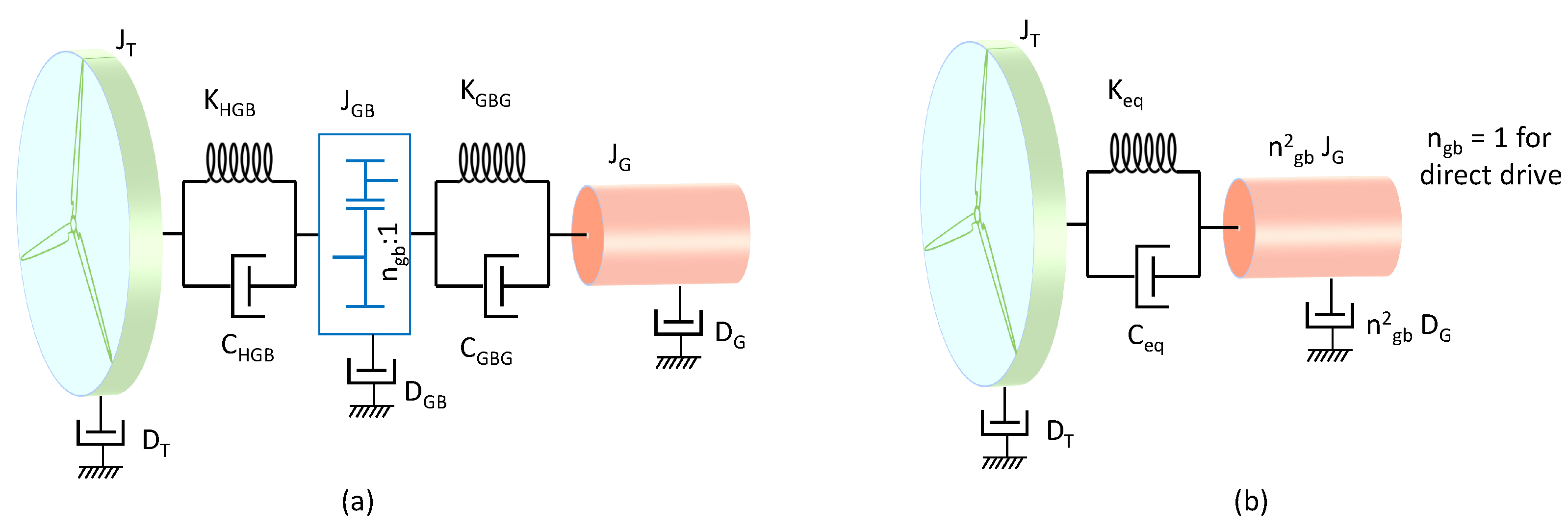
2.6. Modelling the Drive Train

A precise study of the behavior of the drive train dynamics requires a model of five masses [10], relating to the turbine rotor Figure 2b, the minimum requirements of which are outlined in IEC 61400-4. However, as mentioned in Section 2.4, a two-mass model is preferentially used in stability studies. Even for this simplified model, it is very difficult to find data for stiffness or even data regarding the damping of the coupling between the rotor and the generator. In fact, the drive train torsional damping is often estimated, as in [17] for the NREL-5MW reference model, by assuming a relative damping ζ = 0.05 . Hence:
c e q = ζ c c c e q = 0.05 c c
with c c deduced from (38).

2.7. Generator Inertia

The different types of generator used in megawatt WTs are listed in [18] along with their generic characteristics and are resumed in Table 1. Typical speeds, in concordance with [19], appear in the third column. Relationships between the mass and the power of the generator have also been extracted from this reference (fifth column). The data of the remaining columns have been extracted from [20], from [21] and from other scattered catalogs.
The expressions in the last column of Table 1 can also be reached with a constructive and functional analysis of the generators. It is worth mentioning that what appears in this column is the mass of the entire machine and, in fact, only the rotor mass and geometry are required for the inertia. Therefore, the mass of the frame and that of the generator should have been subtracted. As a rule of thumb, many authors assume the same mass for the three components, although the ratio between the mass of the rotor with respect to the stator increases with the number of pairs of poles.
In general, for IGs, the torque and speed are determined, respectively, by the stator current and the voltage. The first magnitude determines the section of Cu and the second, the number of turns; hence, the power increases with the mass of Cu. On the other hand, to achieve a certain torque, Lorentz’s law indicates that the force is proportional to the length of the conductor (that is, the length of the machine and the number of windings that fit in the periphery), while the arm is related to the radius. Consequently, the power will be roughly proportional to the volume of the machine. Assuming that diameter and depth are scaled equally, we have:
Induction generators J M D G 2 P ( 5 / 3 ) H = J Ω G 2 2 P P ( 2 / 3 )
since the speed of the generator rotor depends on its number of pairs of poles which is independent of the power.
For slow synchronous generators, the speed is given by the inverse of the n p p , and this number, in turn, determines the circumference length of the generator rotor.
Ω G 1 n p p 1 D G
On the other hand, an increase in the power of an electric machine implies a roughly proportional increase in weight. Consequently, as far as inertia is concerned, we have:
Direct Drive Synchronous generators J M D G 2 H J Ω G 2 P c t e

3. Results

In this section, various expressions and relationships will be released that link the different aspects relating to blade design: the power of the turbine that would mount the blade, the rotor diameter, the blade length, the blade mass... Subsequently, the results relative to the different elements of the turbine dynamics will be shown, especially the inertia of the blades.

3.1. Expressions Relating to Weight and Blade Length

Each blade model is designed for certain wind conditions which determine its geometry and mass, and therefore, its inertia. The different conditions are included in the IEC 61400 standard, which distinguishes between several classes depending on the average wind speed (IEC Class I, II and III) and turbulence (subclasses A and B). Class IA is the most demanding in terms of design requirements. Table 2 shows a comparison of the average mass of a blade, as a function of wind class and power. An additional class, T, has been created for areas which experience typhoons. Sometimes, Class S is also indicated independently or in combination with another class, in the case of non-standard conditions specified by the manufacturer. Different versions are often based on a blade model, with each one adapted to a certain class.
The left-hand plot of Figure 4 shows the dependence of the mass and the length of the blade on different design classes. Some weight reduction was observed for Class III turbines, but contrary to what is shown in Table 2, there was no significant difference between Class I and Class II turbines.
On the other hand, the experience and trajectory of each blade manufacturer usually leads to the use of a different material and method for its structure. At first, it was mainly polyester resin, reinforced with glass fibers, the matrix of which has been displaced by epoxy resin whose composites exhibit better properties than polyester resin. Both of these are considered to be glass fiber reinforced polymer (GFRP). Later, carbon fiber reinforced polymer (CFRP) was introduced to substitute glass or to be combined to form hybrid glass-carbon blades (Gl-C/Ep) [22,23].
In the right-hand plot of Figure 4, the blades have been classified according to the essential material employed in their manufacture. In this set of study, it was observed that composite materials, based on fibers and polymers, have displaced metals or wood, with a clear predominance of blades using GFRP. For this group, it is difficult to deduce from catalogs whether the matrix is polyester or epoxy. Blades, based on CFRP, appear less frequently and are usually hybrid composites (CFRP/GFRP). For this material, a certain decrease in the weight of the blade is observed. The opposite occurs for steel blades, which are significantly heavier, although it should be mentioned that these are two-blade turbines.
Table 3 lists the relationship between M and L found for every case of study, with M expressed in T and L in m. The rows are divided into three groups according to their capacity, IEC class and material.
The relatively bad correlation (0.865) found in turbines larger than 3 MW, disregarding IEC class or material, indicates that there is great variability due to design conditions and material; therefore, it is preferable to know the IEC class and the material to have a good estimate of the weight, if this is unknown.

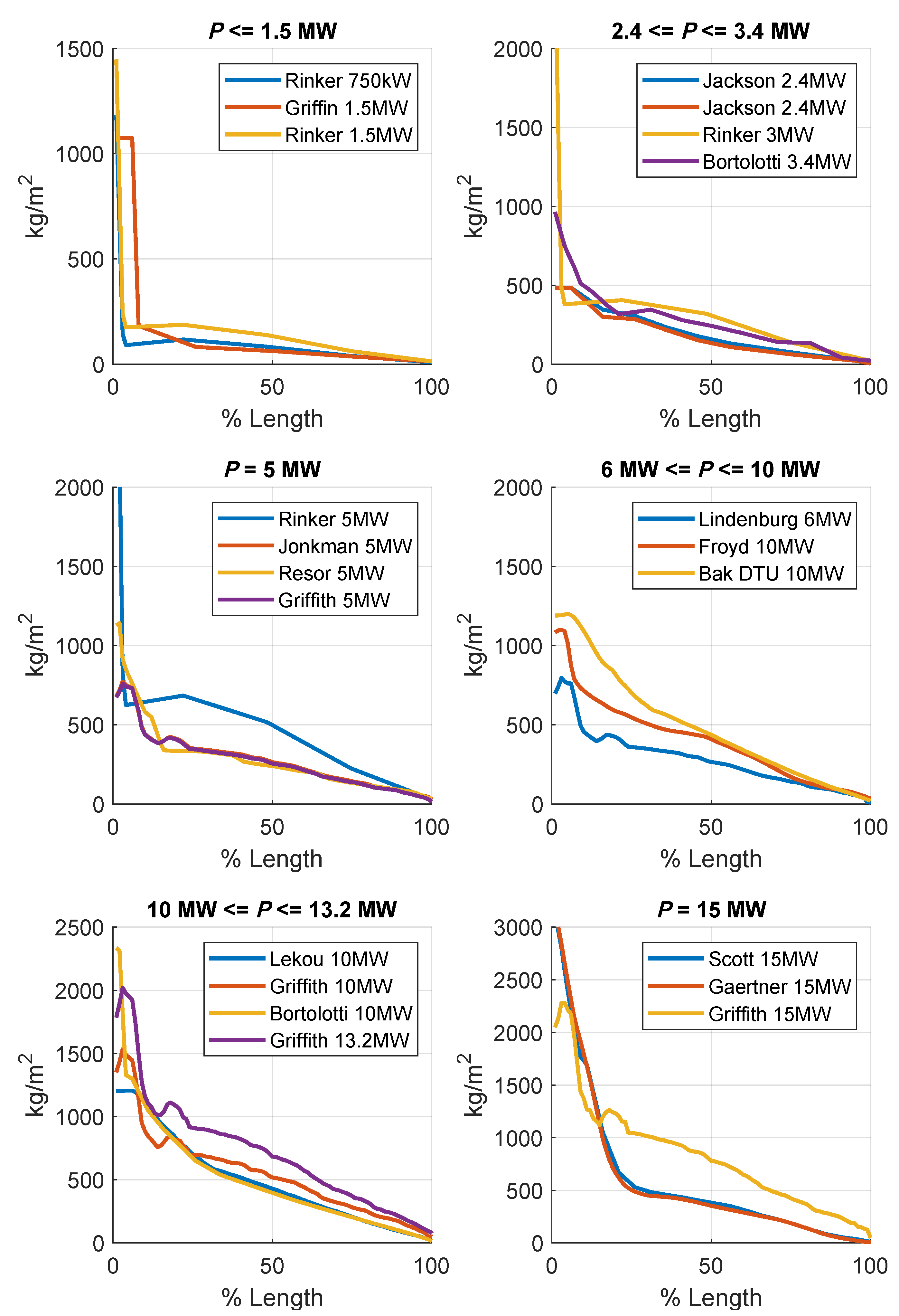
3.2. Inertia Obtained from Density Distribution

The most distinctive aspect of this work is to offer a set of inertia values obtained from the DDs of different blade models found in the literature. This distribution is not arbitrary, but a consequence of a detailed structural and aerodynamical analysis. The resulting data are organized in the Mendeley [16] repository, along with a Matlab script to retrieve the data. From them, the inertia has been calculated for each of the blade models presented, as well as the position of the CoG, with respect to the center of rotation.
Figure 5 represents the mass distribution along the blade for 21 blade models. The data have been interpolated for each model in order to provide 101 values, uniformly separated between 0 and 1, where 0 is the blade root and 1 is its tip.
The result of operating with these data is shown in Table 4. The meaning of each column is the following:
1.
Capacity of the turbine for which the blade is designed.
2.
Maximum rotational speed. This matches the rated rotor speed of the turbine.
3.
Blade mass, as extracted from the reference (up) and calculated by the integration (down).
4.
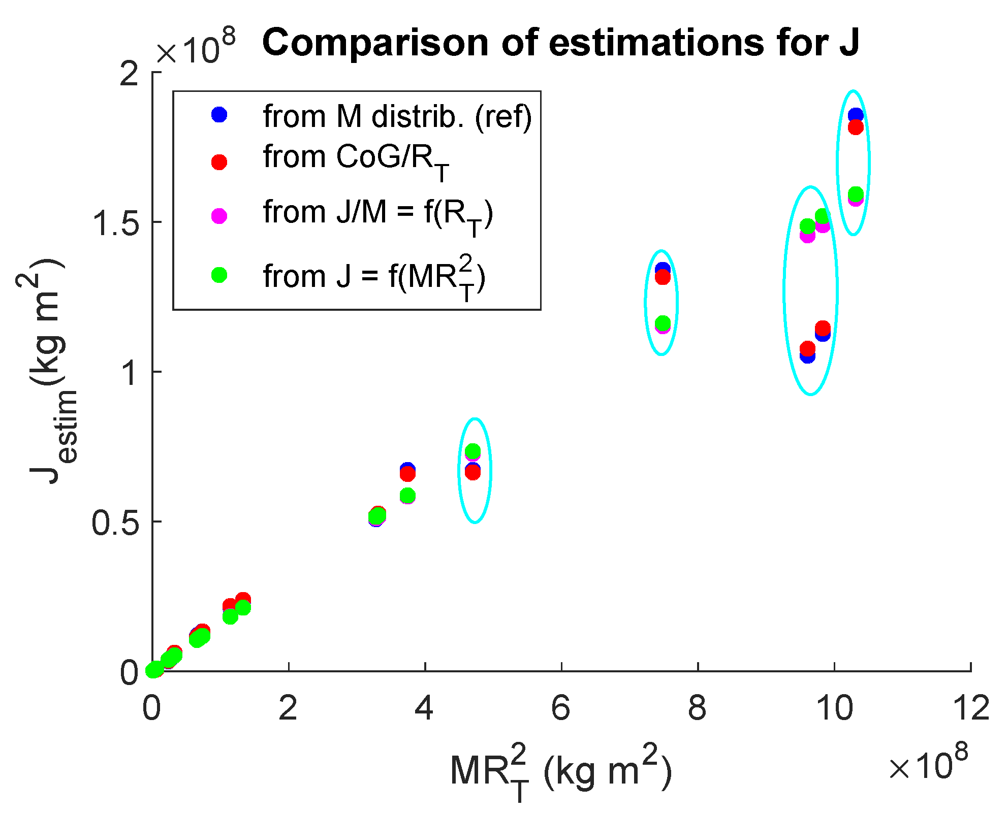
Inertia of the blade, as extracted from the reference (up) and calculated by the integration (down). A value of CoG or inertia appears in cursive when it refers to the blade root instead of the rotation axis.
5.
Inertia of the three blades, as extracted from the reference (up) and calculated by the integration (down). The extracted data have been moved, where necessary, to the rotation axis.
6.
Position of the CoG with respect to the rotation axis, as extracted from the reference (up) and calculated by the integration (down).
7.
Calculated position of the CoG, divided by the the rotor radius.
8.
Value of the coefficient k J = J B / ( M B L B 2 ) .
9.
Time constant of inertia H.
10.
Reference where data have been obtained.
In many cases, the inertia value does not appear as such, but as the “first mass moment of inertia”, as in [24]. In this case, it must be divided by M B . Attention must be paid as to whether the CoG value refers to the axis of rotation or to the blade root. In the latter case, for the purposes of inertia of the rotor as a whole, R h u b must be added. The latter also applies to inertia (also designated as the “second mass moment of inertia”) and (40) should be applied.
Other inertia values obtained from the literature, although without providing the mass distribution, are included in Table 5. Only data originally provided in kg m 2 , not in s, are included.
As discussed previously, there are different airfoils along the blade span, grouped into four regions. The first region, the root, has the assembly structure with the hub and must withstand the greatest moments. It is this zone in which a higher density is observed in kg/m, and this difference is notable from one model to another. In any case, since this region is close to the AoR, its influence on the inertia is minimal.
If one tries to find some type of relationship between the inertia J of the blade, as a function of the mass and the length of the blade, the expressions are obtained with an apparently good correlation. Thus, when looking for a relationship of the type J B / M B = F ( L B ) , it yields:
J B = 0.239 M B L B 1.905
A relationship of the type J B = F ( M B L B 2 ) has also been tested, with the following result:
J B = 0.211 M B L B 2 0.985 .
Figure 6 (in blue) represents the inertia values obtained from the mass distribution extracted from the references in Table 4, which are taken as real values. Shown in purple and green, the direct estimates of inertia from the expressions (45) and (46), are recorded, respectively. It has been observed that, in the case of these estimates, obtained without taking geometry into account, there is a deviation from the estimated values (purple and green points) with respect to the value taken as a reference (blue).
In the following, the blade geometry will be included in the inertia estimation through the CoG position. Accordingly, a more precise estimation of the blade inertia is obtained by comparing columns 7 ( C o G / L ) and 8 ( k J ) of Table 4. This is represented in Figure 7 with a good correlation between them ( r 2 = 0.975 ), in the form:
k J = J B M B ( L B + R h u b ) 2 = J B M B R T 2
and
C o G p u 2 = C o G 2 ( L B + R h u b ) 2 = C o G 2 R T 2 .
From Figure 7, it can be seen that they are related through:
k J = 0.042 + 1.114 C o G 2 R T 2 .
or
J B = M B 0.042 R T 2 + 1.114 C o G 2
The results of applying (50) are observed in Figure 6 as the items with the red marker, and are compared to the results of applying (45) and (46). As can be seen, the values obtained from the CoG (red marker) are very similar to those calculated from the DD (in blue). Consequently, expression (50) allows for a precise estimate of the inertia once the mass, length and CoG positions are known.
It should be mentioned that when the value of ( C o G R H ) / L B is used as abscissa instead of C o G · / R r o t o r , a similar relationship is obtained, although with a somewhat lower correlation ( r 2 = 0.972 ). However, there is no observed dependence between the turbine capacity, identified through the marker colour in Figure 7 and k J .

3.3. Drive Train

Based on data obtained from [20], it can be seen that medium-speed wind turbines use planetary gears, with one or two stages. Clipper wind turbines, with four synchronous generators per turbine, and those that mount the WinDrive system are practically the only high-speed models with two stages. All the others with a speed above 1000 rpm have three stages, mainly combining spur and planetary, and specifically comprise 181 models of 241. There are some other models (37/241) with planetary gears along with helical or spur gears only (7/241) or just planetary (6/241). Each type has its own transmission structure that gives different stiffness constants [43].
The values found are very scarce and, in many cases, the reliability of their origin is questionable. They are represented in Table 6, where the dimensional values are in uppercase and the p.u. values are in lowercase. The parameters are those indicated in Figure 2. Most of these values are in the range specified by Gonzalez-Longatt in [11]: LSS stiffness, K L S S (p.u./ r a d e l ) 0.35–0.70; HSS stiffness, K H S S (p.u./ r a d e l ) (p.u.) 2.00–4.00. In general, the coupling on the slow shaft is less rigid than that on the fast shaft. In addition, within their wide ranges, the turbines with active-stall control typically occupy the upper values and those with pitch control occupy the lower values.

3.4. Hub Inertia

The hub is the weightier rotating component and, therefore, its inertia must be taken into account or at least analyzed. Table 7 lists certain values found in the literature:
Although the weight of the hub is around twice that of a blade, its concentration around the axis of rotation means that the inertia, expressed in s, does not have a representative value with respect to the general dynamics.

3.5. Generator Inertia

This component, although not as heavy as the hub, will add significant inertia to the system dynamics, since, except in the case of direct coupled turbines, there will be a gearbox to accommodate the rotor and generator speeds. Thus, although the inertia of the generator in kg m 2 is not that high, when viewed from the slow axis of the gearbox, its apparent inertia is multiplied by the gear ratio squared. In this case, the time constant is obtained from the expression (26). Table 8 lists certain representative values:
Other values, supplied directly in s, are: H = 0.685 s for a 2 MW DFIG [53]; H = 0.142 s for a 0.6 MW DFIG [47]; H = 2 s for a 0.75 MW DGIG [10]; H = 0.5 s for a 1.5 MW PMSG [49]; H = 0.75 s for a 1.67 MW DFIG [13]; H = 1.150 s for a 2 MW PMSG [54]; H = 0.4 s for a 5 MW DFIG [50].
These values are more significant than those from the hub, and should be considered in dynamic studies. It was also observed that there is a great variability in the value of H, which will prove difficult in extracting some generic law, as the inertia will depend on the constructive characteristics of the rotor, probably whether the generator is an IG or a PMSG.

4. Discussion

4.1. Article Contribution

The main focus of this article has been to provide reliable inertia data for the wind turbine. For this reason, H T values recovered from the bibliographic search have not been included.
An expression has been proposed that quite accurately links inertia to the mass of the blade, its length and the position of the center of gravity, although the latter is only slightly easier to find than the inertia itself. Two expressions have also been proposed, which are very similar in terms of their results and which do not require CoG data, although there is a deviation for some blade models with less conventional geometry.
In order to model the mechanical power transmission dynamics, this work has two additional purposes. The first is to establish an end-to-end dimensionless framework of the mechanical magnitudes that come into play in the turbine dynamics. The second is to collect existing data on the inertia of the remainder of the components and other mechanical parameters, such as stiffness, friction and damping. Since the data found are scarcer, the values in p.u. found in the literature have been incorporated into the review. However, many are not entirely reliable or have not been precisely defined in the base magnitudes of the adimensionalization.

4.2. Limitations and Benefits of the Proposed Work

As already mentioned, the present work provides an expression that presents the designer with a very accurate value of the blade inertia. Its limitation is that one of the arguments required is the position of the CoG. This value is easier to find than the inertia value, but even so, it is not often found for each turbine model.

4.3. Future Work

The aim of future work is to study in depth the characteristics of the coupling between the hub and the generator, especially in the slow shaft for non direct-drive couplings. This will allow to link the values of stiffness and damping more precisely. The constructive characteristics of squirrel cage, wound rotor and PMSGs will also be studied in order to deduce in each case the expressions that link its rated capacity with the rotor weight and, if possible, with its inertia.

Author Contributions

Conceptualization, A.G.G.-R. and J.M.R.-F.; Data curation, A.G.G.-R. and L.M.N.-N.; Formal analysis, A.G.G.-R. and J.M.R.-F.; Investigation, A.G.G.-R. and L.M.N.-N.; Methodology, A.G.G.-R. and L.M.N.-N.; Project administration, A.G.G.-R.; Resources, L.M.N.-N.; Software, A.G.G.-R. and L.M.N.-N.; Supervision, J.M.R.-F.; Validation, A.G.G.-R. and L.M.N.-N.; Visualization, A.G.G.-R. and J.M.R.-F.; Writing—original draft, A.G.G.-R.; Writing—review and editing, J.M.R.-F. All authors have read and agreed to the published version of the manuscript.

Funding

This research received no external funding.

Institutional Review Board Statement

Not applicable.

Data Availability Statement

Data with the DD and other data related to blade models can be found in [16].

Conflicts of Interest

The authors declare no conflict of interest.

Abbreviations

The following abbreviations are used in this manuscript. They can appear as subscript or superscript for some variables or magnitudes
AoRAxis of rotation
BBlade
CoGCenter of gravity
DDDensity distribution
DFIGDoubly-fed induction generator
eqEquivalent of m2 and turbine
GGenerator
GBGearbox
GBGShaft joining gearbox and generator
HGBShaft joining hub and gearbox
HSSHigh-speed shaft
IGInduction generator
LSSLow-speed shaft
m2Components at the high-speed side
PTurbine rated capacity
PMSGPermanent magnet synchronous generator
TTurbine or turbine rotor
WWind
WTWind turbine
The following variables and parameters are used in this manuscript:
Magnitude
Symbol [units]Referred to base [units]
Rotational speed Ω r a d / s ω r a d e l / s
TorqueT N m t p . u .
Twist angle Θ r a d Θ r a d e l
InertiaJ k g m 2 H s
Mutual dampingC N · m · s r a d m e c c p . u .
Shelf dampingD N · m · s r a d m e c d p . u .
Torsion stiffnessK N · m r a d m e c k p . u . r a d e l
E k Kinetic energy J
fGrid frequency [Hz]
PTurbine rated capacity [W, also MW when explicitly specified]
k J Shape coefficient, defined in (47)
n p p Number of pole pairs
n g b Gearbox ratio
rCorrelation index
ζ Relative damping

References

  1. Li, H.; Zhao, B.; Yang, C.; Chen, H.W.; Chen, Z. Analysis and estimation of transient stability for a grid-connected wind turbine with induction generator. Renew. Energy 2011, 36, 1469–1476. [Google Scholar] [CrossRef]
  2. Fernández-Guillamón, A.; Vigueras-Rodríguez, A.; Molina-García, Á. Analysis of power system inertia estimation in high wind power plant integration scenarios. IET Renew. Power Gener. 2019, 13, 2807–2816. [Google Scholar] [CrossRef]
  3. Miao, L.; Wen, J.; Xie, H.; Yue, C.; Lee, W.J. Coordinated Control Strategy of Wind Turbine Generator and Energy Storage Equipment for Frequency Support. IEEE Trans. Ind. Appl. 2015, 51, 2732–2742. [Google Scholar] [CrossRef]
  4. He, X.; Geng, H.; Mu, G. Modeling of wind turbine generators for power system stability studies: A review. Renew. Sustain. Energy Rev. 2021, 143, 110865. [Google Scholar] [CrossRef]
  5. Ekanayake, J.; Jenkins, N. Comparison of the response of doubly fed and fixed-speed induction generator wind turbines to changes in network frequency. IEEE Trans. Energy Convers. 2004, 19, 800–802. [Google Scholar] [CrossRef]
  6. Morren, J.; Pierik, J.; de Haan, S.W. Inertial response of variable speed wind turbines. Electr. Power Syst. Res. 2006, 76, 980–987. [Google Scholar] [CrossRef]
  7. Tielens, P.; Van Hertem, D. The relevance of inertia in power systems. Renew. Sustain. Energy Rev. 2016, 55, 999–1009. [Google Scholar] [CrossRef]
  8. Gonzalez-Longatt, F.M. Effects of the synthetic inertia from wind power on the total system inertia: Simulation study. In Proceedings of the 2012 2nd International Symposium On Environment Friendly Energies And Applications, Newcastle Upon Tyne, UK, 25–27 June 2012; pp. 389–395. [Google Scholar] [CrossRef]
  9. Fernández-Guillamón, A.; Gómez-Lázaro, E.; Muljadi, E.; Molina-García, Á. Power systems with high renewable energy sources: A review of inertia and frequency control strategies over time. Renew. Sustain. Energy Rev. 2019, 115, 109369. [Google Scholar] [CrossRef]
  10. Girsang, I.P.; Dhupia, J.S.; Muljadi, E.; Singh, M.; Pao, L.Y. Gearbox and drivetrain models to study dynamic effects of modern wind turbines. IEEE Trans. Ind. Appl. 2014, 50, 3777–3786. [Google Scholar] [CrossRef]
  11. Gonzalez-Longatt, F.; Regulski, P.; Novanda, H.; Terzija, P. Effect of the shaft stiffness on the inertial response of the fixed speed wind turbines and its contribution to the system inertia. In Proceedings of the 2011 International Conference on Advanced Power System Automation and Protection, Beijing, China, 16–20 October 2011; Volume 2. [Google Scholar] [CrossRef]
  12. Akhmatov, V.; Knudsen, H. An aggregate model of a grid connected, large scale, offshore wind farm for power stability investigations - importance of windmill mechanical system. Electr. Power Energy Syst. 2002, 24, 709–717. [Google Scholar] [CrossRef]
  13. Rahimi, M. Drive train dynamics assessment and speed controller design in variable speed wind turbines. Renew. Energy 2016, 89, 716–729. [Google Scholar] [CrossRef]
  14. Frøyd, L.; Dahlhaug, O.G. Rotor design for a 10 MW offshore wind turbine. Proc. Int. Offshore Polar Eng. Conf. 2011, 8, 327–334. [Google Scholar]
  15. Schubel, P.; Crossley, R. Wind Turbine Blade Design Review. Wind Eng. 2012, 36, 365–388. [Google Scholar] [CrossRef]
  16. Gonzalez-Rodriguez, A.G. Review of mass distribution of wind turbine blades. Mendeley Data 2023, V1. [Google Scholar] [CrossRef]
  17. Jonkman, J.; Butterfield, S.; Musial, W.; Scott, G. Definition of a 5-MW reference wind turbine for offshore system development. Technical report, NREL, 2009. Available online: https://doi.org/https://doi.org/10.2172/947422 (accessed on 1 June 2023).
  18. Bywaters, G.; John, V.; Lynch, J.; Mattila, P.; Norton, G.; Stowell, J.; Salata, M.; Labath, O.; Chertok, A.; Hablanian, D. Northern Power Systems WindPACT Drive Train Alternative Design Study Report. Technical Report October 2004, NREL, 2004. Available online: http://www.osti.gov/servlets/purl/15007774/ (accessed on 1 June 2023).
  19. Fingersh, L.; Hand, M.; Laxson, A. Wind Turbine Design Cost and Scaling Model. NREL 2006, 29, 1–43. [Google Scholar]
  20. Windturbines Database. Available online: https://en.wind-turbine-models.com/turbines (accessed on 1 June 2023).
  21. Available online: https://4coffshore.com (accessed on 1 June 2023).
  22. Lekou, D.J.; Cres, D.C. Results of the benchmark for blade structural models. Technical Report November 2012, InnWind.EU, 2013. Available online: https://orbit.dtu.dk/en/publications/results-of-the-benchmark-for-blade-structural-models-part-a (accessed on 1 June 2023).
  23. Jackson, K.J.; Zuteck, M.D.; Van Dam, C.P.; Standish, K.J.; Berry, D. Innovative design approaches for large wind turbine blades. Wind Energy 2005, 8, 141–171. [Google Scholar] [CrossRef]
  24. Rinker, J.; Dykes, K. WindPACT Reference Wind Turbines, 2018. Available online: https://www.nrel.gov/docs/fy18osti/67667.pdf (accessed on 1 June 2023).
  25. Griffin, D.A. Evaluation of Design Concepts for Adaptive Wind Turbine Blades. Technical report, Sandia National Lab, 2002. Available online: https://doi.org/10.2172/801399 (accessed on 1 June 2023).
  26. Bortolotti, P.; Tarres, H.C.; Dykes, K.; Merz, K.; Sethuraman, L.; Verelst, D.; Zahle, F. IEA Wind Task 37 on Systems Engineering in Wind Energy–WP2.1 Reference Wind Turbines. Available online: https://github.com/IEAWindTask37/IEA-3.4-130-RWT/tree/master/hawc2/data, (accessed on 1 June 2023).
  27. Resor, B.R. Definition of a 5MW/61.5 m wind turbine blade reference model. Albuquerque, New Mex. USA, Sandia Natl. Lab. SAND2013-2569 2013 2013, 2013, 50. [Google Scholar]
  28. Lindenburg, C. Aeroelastic Analysis of the LMH64-5 Blade Concept; Technical Report June; Energy Research Centre of the Netherlands ECN: Petten, The Netherlands, 2003. [Google Scholar]
  29. Bak, C.; Zahle, F.; Bitsche, R.; Kim, T.; Yde, A.; Henriksen, L.C.; Hansen, M.H.; Blasques, J.P.A.A.; Gaunaa, M.; Natarajan, A. The DTU 10-MW Reference Wind Turbine. Available online: https://github.com/Seager1989/DTU10MW_FAST_LIN/blob/main/Rotor/DTU_10MW_ElastoDyn_Blades.dat (accessed on 1 July 2023).
  30. Bortolotti, P.; Tarres, H.C.; Dykes, K.; Merz, K.; Sethuraman, L.; Verelst, D.; Zahle, F. IEA Wind Task 37 on Systems Engineering in Wind Energy–WP2.1 Reference Wind Turbines. Available online: https://github.com/IEAWindTask37/IEA-10.0-198-RWT/tree/master/hawc2/data (accessed on 1 June 2023).
  31. Griffith, D.T.; Ashwill, T.D. The Sandia 100-meter All-glass Baseline Wind Turbine Blade: SNL100-00, 2011. https://energy.sandia.gov/wp-content/gallery/uploads/113779A.pdf. (accessed on 1 June 2023).
  32. IEA Wind - Offshore Reference Wind-15MW. Data. Available online: https://github.com/IEAWindTask37/IEA-15-240-RWT/blob/master/HAWC2/IEA-15-240-RWT/IEA_15MW_RWT_Blade_st_FPM.st, (accessed on 1 July 2023).
  33. Gaertner, E.; Rinker, J.; Sethuraman, L.; Zahle, F.; Anderson, B.; Barter, G.; Abbas, N.; Meng, F.; Bortolotti, P.; Skrzypinski, W.; et al. IEA Wind TCP Task 37, NREL Definition of the IEA Wind 15-Megawatt Offshore Reference Wind Turbine, 2020. Available online: https://www.nrel.gov/docs/fy20osti/75698.pdf (accessed on 1 June 2023).
  34. Scott, S.; Greaves, P.; Macquart, T.; Pirrera, A. Comparison of blade optimisation strategies for the IEA 15MW reference turbine. J. Phys. Conf. Ser. 2022, 2265. [Google Scholar] [CrossRef]
  35. Sørensen, P.; Madsen, P.; Vikkelsø, A.; Jensen, K.; Fathima, K.; Unnikrishnan, A.; Lakaparampil, Z. Power quality and integration of wind farms in weak grids in India, 2000. Available online: https://orbit.dtu.dk/en/publications/power-quality-and-integration-of-wind-farms-in-weak-grids-in-indi (accessed on 1 June 2023).
  36. Carrillo, C.; Feijoo, A.; Cidras, J.; Gonzalez, J. Power fluctuations in an isolated wind plant. IEEE Trans. Energy Convers. 2004, 19, 217–221. [Google Scholar] [CrossRef]
  37. Chedid, R.; F. Mrad. Intelligent Control of a Class of Wind Energy Conversion Systems. IEEE Trans. Energy Convers. 1999, 14, 1597–1604. [Google Scholar] [CrossRef]
  38. Garcia, H.; Segundo, J.; Rodríguez, O.; Campos-Amezcua, R.; Jaramillo, O. Harmonic Modelling of the Wind Turbine Induction Generator for Dynamic Analysis of Power Quality. Energies 2018, 11, 104. [Google Scholar] [CrossRef]
  39. Kayikçi, M.; Milanović, J.V. Dynamic contribution of DFIG-based wind plants to system frequency disturbances. IEEE Trans. Power Syst. 2009, 24, 859–867. [Google Scholar] [CrossRef]
  40. Licari, J.; Ekanayake, J.; Moore, I. Inertia response from full-power converter-based permanent magnet wind generators. J. Mod. Power Syst. Clean Energy 2013, 1, 26–33. [Google Scholar] [CrossRef]
  41. Harrison, S.; Papadopoulos, P.N.; Silva, R.D.; Kinsella, A.; Gutierrez, I.; Egea-Alvarez, A. Impact of Wind Variation on the Measurement of Wind Turbine Inertia Provision. IEEE Access 2021, 9, 122166–122179. [Google Scholar] [CrossRef]
  42. Mercado-Vargas, M.; Gómez-Lorente, D.; Rabaza, O.; Alameda-Hernandez, E. Aggregated models of permanent magnet synchronous generators wind farms. Renew. Energy 2015, 83, 1287–1298. [Google Scholar] [CrossRef]
  43. Peeters, J.L.M.; Vandepitte, D.; Sas, P. Analysis of internal drive train dynamics in a wind turbine. Wind Energy 2006, 9, 141–161. [Google Scholar] [CrossRef]
  44. Petru, T.; Thiringer, T. Modeling of wind turbines for power system studies. IEEE Transactions on Power Systems 2002, 17, 1132–1139. [Google Scholar] [CrossRef]
  45. Papathanassiou, S.; Papadopoulos, M. Dynamic behavior of variable speed wind turbines under stochastic wind. IEEE Trans. Energy Convers. 1999, 14, 1617–1623. [Google Scholar] [CrossRef]
  46. Vilar, C.; Usaola, J.; Amarís, H. A frequency domain approach to wind turbines for flicker analysis. IEEE Trans. Energy Convers. 2003, 18, 335–341. [Google Scholar] [CrossRef]
  47. Rodriguez, J.; Fernandez, J.; Beato, D.; Iturbe, R.; Usaola, J.; Ledesma, P.; Wilhelmi, J. Incidence on power system dynamics of high penetration of fixed speed and doubly fed wind energy systems: Study of the Spanish case. IEEE Trans. Power Syst. 2002, 17, 1089–1095. [Google Scholar] [CrossRef]
  48. Rahim, Y.; Al-Sabbagh, A. Controlled power transfer from wind driven reluctance generator. IEEE Trans. Energy Convers. 1997, 12, 275–281. [Google Scholar] [CrossRef]
  49. Xi, J.; Geng, H.; Yang, G.; Ma, S. Inertial response analysis of PMSG-based WECS with VSG control. J. Eng. 2017, 2017, 897–901. [Google Scholar] [CrossRef]
  50. Mancilla-David, F.; Domínguez-García, J.L.; De Prada, M.; Gomis-Bellmunt, O.; Singh, M.; Muljadi, E. Modeling and control of Type-2 wind turbines for sub-synchronous resonance damping. Energy Convers. Manag. 2015, 97, 315–322. [Google Scholar] [CrossRef]
  51. Kooijman, H.; Lindenburg, C.; Winkelaar, D.; Hooft. DOWEC 6 MW PRE-DESIGN Aero-elastic modelling of the DOWEC 6 MW pre-design in PHATAS Acknowledgement/Preface. 2003. Available online: https://api.semanticscholar.org/CorpusID:111438322 (accessed on 1 June 2023).
  52. Sethuraman, L.; Xing, Y.; Gao, Z.; Venugopal, V.; Mueller, M.; Moan, T. A 5MW direct-drive generator for floating spar-buoy wind turbine: Development and analysis of a fully coupled Mechanical model. Proc. Inst. Mech. Eng. Part A J. Power Energy 2014, 228, 718–741. [Google Scholar] [CrossRef]
  53. Zhao, M.; Yuan, X.; Hu, J. Modeling of DFIG Wind Turbine Based on Internal Voltage Motion Equation in Power Systems Phase-Amplitude Dynamics Analysis. IEEE Trans. Power Syst. 2018, 33, 1484–1495. [Google Scholar] [CrossRef]
  54. Li, Y.; Xu, Z.; Wong, K.P. Advanced Control Strategies of PMSG-Based Wind Turbines for System Inertia Support. IEEE Trans. Power Syst. 2017, 32, 3027–3037. [Google Scholar] [CrossRef]
Figure 1. Typical components in a wind turbine drive train.
Machines 11 00908 g001
Figure 2. (a) Schematic diagram of the traditional three-mass and (b) two-mass equivalent model of a wind turbine. In the two-mass equivalent model, HSS-side values are translated to the LSS-side.
Machines 11 00908 g002
Figure 3. The position of the CoG with respect to the blade root is the position with respect to the AoR summed to the hub radius.
Machines 11 00908 g003
Figure 4. Blade mass as a function of the length: (a) for different IEC classes; (b) for different materials.
Machines 11 00908 g004
Figure 5. Mass distribution along the blade for different models. The position along the blade is normalized by dividing the blade length, starting from the root. The following references apply: Rinker 0.75/1.5/3/5MW [24]; Griffin 1.5 MW [25]; Jackson 2.4 Carbon/E-glass [23], Bortolotti 3.4 MW [26], Jonkman 5 MW [17], Resor 5 MW [27], Lindenburg 6 MW [28], DTU 10 MW [29], Bortolotti 10 MW [30], Lekou 10 MW [22], Griffith 10/13.2/15 MW [31], Froyd 10MW [14], Scott 15MW [32], Gaertner 15 MW [33].
Machines 11 00908 g005
Figure 6. Comparison of several estimates to obtain J with respect to the value calculated from the DD (blue). In purple, the estimate from (45). In green, the estimate from (46). In red, the estimate from kJ obtained from the CoG (50).
Machines 11 00908 g006
Figure 7. Correlation between the position of the CoG and the inertia, obtained from the mass distributions found in the literature. The value, L, is half the rotor diameter.
Machines 11 00908 g007
Table 1. Types of generators and the corresponding coupling to the turbine rotor.
TypePole PairsSpeedDrive TrainRatio P (kW) M (kg)
Squirrel cage induction2 ÷ 31000 ÷ 1800 rpmThree stages, n G B  > 502  M = 10.51 P 0.92
Wound rotor induction2 ÷ 31000 ÷ 1800 rpmThree stages, n G B  > 50 M = 10.51 P 0.92
Synchronous5 ÷ 12300 ÷ 600 rpm 1Two stages n G B  = 12 ÷ 45 M = 6.47 P 0.92
Synchronous10 ÷ 40100 ÷ 160 rpmOne stage n G B  = 10 M = 6.47 P 0.92
Synchronous200 ÷ 35010 ÷ 20Direct-drive M = 661 ( P / Ω T ) 0.61
1 Manufacturers as Clipper, Eno Energy or Catum mount fast synchronous machines up to 1600 rpm. 2 The exponent 0.92 for induction generators is coherent with the statement that M ∝ P.
Table 2. Comparison of blade mass per length depending on the IEC wind class.
Class I (kg/m)Class II (kg/m)Class III (kg/m)Class IV (kg/m)Ref
1.5 MW163159143 [22]
2 MW168145131 [22]
3 MW201.7164.8144.1119.0[23]
Table 3. Expressions linking M in kg and L in m.
Designed forExpressionCorrelation r 2
P < 3 M W M = 8.6 L 1.834 0.936
P 3 M W M = 5.5 L 1.968 0.865
IEC Class I M = 4.2 L 2.039 0.959
IEC Class II M = 10.1 L 1.801 0.944
IEC Class III M = 2.5 L 2.1108 0.994
GFRP M = 7.04 L 1.9027 0.961
Hybrid M = 14.8 L 1.631 0.909
Table 4. Values relative to the mass, length and inertia of several blade models extracted from the literature, and compared with the values obtained from the DD appearing in the corresponding reference.
MW Ω T (rpm)M (kg)1  J bl
(kg m 2 )
J rt
(kg m 2 )
1  CoG (m) CoG ( % ) k J H rt (s)Ref.
0.75028.651941
1940
1.806  × 10 5 2.180  × 10 5 6.786  × 10 5 6.540  × 10 5 8.770 8.7640.3510.1803.924[24]
1.50022.502530
4408
-
6.360  × 10 5
-
1.908  × 10 6
-
8.607
0.2340.1073.531[25]
1.50020.464336
4332
7.985  × 10 5 9.653  × 10 5 3.003  × 10 6 2.896  × 10 6 12.47 12.460.3560.1824.432[24]
2.400-8799
9560
-
3.910  × 10 6
-
1.173  × 10 7
-
16.71
0.3210.151-[23]
2.400-7920
8721
-
3.388  × 10 6
-
1.016  × 10 7
-
16.16
0.3110.144-[23]
3.00014.4713,238
13,230
5.012  × 10 6 6.070  × 10 6 1.884  × 10 7 1.821  × 10 7 18.12 18.110.3660.1876.968[24]
3.4008.67916,441
16,466
-
1.179  × 10 7
-
3.537  × 10 7
-
21.78
0.3350.1694.297[26]
5.00011.1927,854
27,880
1.748  × 10 7 2.121  × 10 7 6.579  × 10 7 6.362  × 10 7 23.42 23.380.3650.1868.737[24]
5.00012.1017,740
16,838
1.178  × 10 7 1.216  × 10 7 3.896  × 10 7 3.648  × 10 7 21.98 21.990.3490.1825.857[17]
5.00011.8417,700
17,012
1.178  × 10 7 1.159  × 10 7 3.876  × 10 7 3.477  × 10 7 0.500 20.770.3300.1725.348[27]
5.00012.1017,740
16,430
-
1.158  × 10 7
-
3.474  × 10 7
20.50 21.700.3440.1785.578[31]
6.00011.8417,334
17,337
1.284  × 10 7 1.330  × 10 7 3.850  × 10 7 3.990  × 10 7 -
22.97
0.3530.1815.115[28]
10.00012.9527,200
26,773
-
2.351  × 10 7
-
7.053  × 10 7
-
24.75
0.3490.1756.485[14]
10.0009.600-
41,699
-
5.163  × 10 7
-
1.549  × 10 8
-
28.89
0.3240.1567.827[29]
10.0009.60042,363
41,620
- 5.072  × 10 7 -
1.522  × 10 8
31.60 28.610.3220.1557.690[22]
10.0008.56050,184
47,104
-
6.714  × 10 7
-
2.014  × 10 8
29.00 30.910.3470.1808.092[31]
10.0008.68047,700
47,943
-
6.717  × 10 7
-
2.015  × 10 8
-
29.57
0.2990.1438.325[30]
13.2007.44076,402
71,234
-
1.340  × 10 8
-
4.020  × 10 8
33.40 35.520.3470.1799.244[31]
15.0007.56068,415
67,003
-
1.126  × 10 8
-
3.378  × 10 8
-
31.34
0.2590.1157.058[34]
15.0007.56065,250
65,417
- 1.053  × 10 8 -
3.160  × 10 8
2.970 30.400.2510.1106.603[33]
15.0006.99092,131
86,626
-
1.855  × 10 8
-
5.565  × 10 8
35.60 37.870.3470.1809.939[31]
1 A value of CoG or inertia appears in cursive when it refers to the blade root instead of the rotation axis.
Table 5. Other values relating to the mass, length and inertia of several blade models extracted from the literature.
MW Ω rot (rpm) n GB J ( kg · m 2 )H (s)Ref.
0.22542.7423.40:166,0002.937[35]
0.22541.0023.40:166,0582.706[36]
0.35019.2121.81:13.500  × 10 5 2.023[37]
0.90022.2267.50:11.600  × 10 6 4.814[38]
1.27020.0090.00:13.716  × 10 6 6.417[39]
2.00018.0083.33:16.029  × 10 6 5.355[40]
3.00016.673.00:11.300  × 10 7  6.600 1[41]
5.00015.001.00:12.530  × 10 7 6.243 2[42]
1 A direct drive is claimed in the article, but this would lead to a tip speed of 227 m/s. H has been obtained assuming a tip speed of 76 m/s. 2 The number of poles found in the reference is 200, but with this value, the tip speed is 196 m/s. It has been assumed that 200 is the number of pole pairs.
Table 6. Values for the drive train components of Figure 2, obtained from the literature. Values in cursive are in pu or pu/el.rad.
MW Ω T (rpm) n GB K HGB (Nm/rad) k HGB (pu/el.rad) K GBG (Nm/rad) k HGBG (pu/el.rad) C HGB / C GBG or C GB (Nms/rad) c HGB / c GBG or c GB (pu) D T / D GB / D G (Nms/rad) d T / d GB / d G (pu)Ref.
0.18042.0024-2700.0
0.52
- / -- / - / -[44]
0.20057.6926--3.500/10.000.022/0.020/0.010[45]
0.22542.74235.10  × 10 6
1.4
--/--/-/-[35]
0.22541.0023-2242.0
0.33
-/-334/-/0.61 0.027/-/0.027[36]
0.33034.00-3.1812.30132.19/-0.004/-/0.004[46]
0.500--54.81834.13.500/10.000.022/0.022/0.035[11]
0.600--50.01834.11.000/10.000.005/0.022/0.005[47]
0.75028.65631.30  × 10 8
4.1
-2.78  × 10 5
3.3
-/-/-[24]
0.90022.22686.00  × 10 7
1.1
-1.00  × 10 6
6
-/-/-[38]
1.00041.7822-1.00  × 10 6
24
-/--/-/-[48]
1.27020.00902.74  × 10 8
2.5
-5.02  × 10 5
1.7
-/-/-[39]
1.50020.46884.83  × 10 8
3.9
-1.36  × 10 6
4.2
-/-/-[24]
1.50020.701.02.00--/--/-/-[49]
1.67016.00750.60-1.200-/-/-[13]
2.00018.00831.60  × 10 8
0.9
-2.50  × 10 5
0.44
-/-/-[40]
3.00014.47124.41.04  × 10 9
2.1
-4.99  × 10 6
3.8
-/-/-[24]
5.00012.10978.68  × 10 8
0.74
-6.22  × 10 6
2/-
-/-/-[17]
5.00011.19160.82.30  × 10 9
1.7
-1.49  × 10 7
4.1
-/-/-[24]
5.00012.37145.50.30-0.00372-/-/-[50]
6.00011.84933.29  × 10 8
0.22
2.78  × 10 6
16
-/--/-/-[51]
1 The values, K L S S and K H S S in [46] have been divided into 2 π f = 314 rad / s , because the values were given in p.u. instead of p.u./el.rad. 2 The value of C G B in [50] has been multiplied by 2 π f = 377 rad / s , because the values were given in p.u. s/el.rad, instead of p.u., although these are still very low.
Table 7. Values for hub inertia obtained from the literature.
MW Ω rot (rpm) n GB J ( kg · m 2 )H (s)Ref.
0.75028.6562.832:151600.031[24]
1.50020.4687.965:12.998  × 10 4 0.046[24]
3.00014.47124.407:11.980  × 10 5 0.076[24]
5.00011.19160.85:16.685  × 10 5 0.092[24]
5.00012.1097.1:11.160  × 10 5 0.019 1[31]
5.00012.1097.1:11.159  × 10 5 0.019 1[17]
6.00011.8492.873:15.070  × 10 4 0.006[51]
10.0008.560137.256:14.640  × 10 5 0.019 1[31]
13.2007.440157.918:18.120  × 10 5 0.019 1[31]
15.0006.990168.084:11.040  × 10 6 0.019 1[31]
1 The references of [31] are equal to one another and are equal to that of [17] since, for this study, the NREL 5 MW model has been taken as a reference and the mass moments of inertia were scaled with the fourth power of the diameter scale factor, which in turn inversely determines the speed of rotation.
Table 8. Values of generator inertia obtained from the literature.
MW Ω rot (rpm) n GB J ( kg · m 2 )H (s) n pp f (Hz)Ref.
0.18042.0023.75:14.5000.1363-[44]
0.22541.0023.40:110.000.224350[36]
0.75028.6562.80:116.650.394260[24]
0.90022.2267.50:135,184 10.106250[38]
1.27020.0090.00:184.081.1762-[39]
1.50020.4688.00:156.440.669260[24]
2.00018.0083.33:1416.62.5702-[40]
3.00014.47124.40:1177.91.053260[24]
3.00016.673.00:1 21.400  × 10 6 6.3976050[41]
5.00012.1097.10:1534.10.8093-[17]
5.00011.19160.80:1438.91.558260[24]
5.00012.1097.10:1534.10.8093-[31]
5.00012.101.00:13.790  × 10 5 0.061248.0-[52]
10.0008.560137.26:121401.6203-[31]
13.2007.440157.92:137402.1453-[31]
15.0006.990168.08:148002.4223-[31]
1 The value seems to refer to the LSS and, consequently, expression (22) has been used to obtain H. 2 Appears as a direct drive, but with n G B = 1, the tip speed is 227 m/s. Assuming n G B = 3 , the tip speed is 75, which is more feasible. The value of J G has been correspondingly divided by n G B 2 .
Disclaimer/Publisher’s Note: The statements, opinions and data contained in all publications are solely those of the individual author(s) and contributor(s) and not of MDPI and/or the editor(s). MDPI and/or the editor(s) disclaim responsibility for any injury to people or property resulting from any ideas, methods, instructions or products referred to in the content.

