Article

Multivariable Linear Position Control Based on Active Disturbance Rejection for Two Linear Slides Coupled to a Mass

by
Fabio Abel Gómez Becerra
1,
Jonathan Villanueva Tavira
2,
Héctor Miguel Buenabad Arias
2,
Andrés Blanco Ortega
2,*,
Estela Sarmiento Bustos
3,
Manuela Calixto Rodríguez
3 and
Jorge Salvador Valdez Martinez
3
1
TecNM/Instituto Tecnológico José Mario Molina Pasquel y Henríquez Campus Puerto Vallarta, Puerto Vallarta 48338, Jalisco, Mexico
2
TecNM/Centro Nacional de Investigación y Desarrollo Tecnológico, Cuernavaca 62490, Morelos, Mexico
3
Division Académica de Mecánica Industrial, Universidad Tecnológica Emiliano Zapata del Estado de Morelos, Av. Universidad Tecnológica 1, Palo Escrito, Emiliano Zapata 62765, Morelos, Mexico
*
Author to whom correspondence should be addressed.
Machines 2023, 11(9), 889; https://doi.org/10.3390/machines11090889
Submission received: 24 July 2023 / Revised: 23 August 2023 / Accepted: 30 August 2023 / Published: 5 September 2023
(This article belongs to the Special Issue New Trends in Robotics, Automation and Mechatronics)

Abstract

:
Active Disturbance Rejection Control (ADRC) is a promising approach that has emerged to deal with uncertainties, which has received many practical applications in motion controls. This paper presents a multivariable controller for active disturbance rejection (ADR) based on an extended state linear observer for tracking the linear position trajectory of a mass moved by two linear slides, each one driven by a DC motor. The linear extended state observer is used to estimate the endogenous and exogenous disturbances of the system, which are assumed to be unknown, but bounded. Therefore, the feedback system prevents each actuator from operating at different forward speeds, and thus a synchronization between the two actuators is achieved by moving the common mass smoothly. The simulation and the experimental results show the effectiveness and robustness of the controller proposal when moving the mass with both actuators.

1. Introduction

At present, the use of multivariable control for different linear and non-linear systems of the electrical, electromechanical and renewable energy types has been widely accepted to solve very specific tasks in terms of controlling the physical variables of the system for a desired point or for a desired trajectory; this can be found in different articles previously published in [1,2,3]. In [1], use is made of the differential flatness property to calculate the desired trajectories of each of the outputs of interest to regulate the non-linear system “double dc/dc converter type reducer coupled to the motor of dc”. In this work, a smooth monitoring of the voltage at the output of the first converter is carried out and at the same time, a smooth monitoring of the angular speed of the motor is carried out. This is achieved by means of a multivariable control based on passivity for the non-linear system proposed.
On the other hand, in [2], a multivariable control by active disturbance rejection is proposed to regulate the angular velocity in the Permanent Magnet Synchronous Motor (PMSM). In this work, they perform a smooth monitoring of the angular speed of the motor and at the same time the current is regulated in its direct component in the d-q coordinates of the non-linear system. Also, it proposes the use of ultra-models that consider the exogenous and endogenous disturbances present in the systems and in combination with a control technique by active rejection of disturbances based on high-gain extended observers for differentially flat nonlinear systems, applied to synchronous motor control [4].
In [3], an angular speed driver of a three-phase induction motor is proposed, where the dc source of the inverter is provided by a boost-type DC/DC converter, which is fed from an array of photovoltaic solar panels. The speed booster uses a boost converter, which regulates its input and output voltage through a passive controller in combination with an algebraic estimator, in order for it to work at the maximum power point, and thereby provide the required voltage to the inverter that drives the motor. While to regulate the speed to the induction motor a field oriented angular velocity smooth tracking control is used.
On the other hand, active disturbance rejection control (ADRC) allows to efficiently solve the control problem for highly disturbed linear and nonlinear dynamic systems, where many of them are designed using the differential flatness property (controllability and observability). Some of these dynamic systems are differentially flat, and others are not; hence, it is necessary to resort to a partial linearization at least and in the last of the cases to an approximate linearization to be able to make use of this property and thus be able to design the ADRC based on extended state observers [5].
In [6], the authors use a controller for active disturbance rejection based on a GPI observer to regulate the output voltage and balance the currents of converters connected in parallel, DC/DC Buck–Parallel Converter.
One of the great advantages of the ADRC approach is that it does not require information from each of the plants when they are dynamically interacting with each other. The idea is that each subsystem takes into account its uncertainties derived from: (1) unknown non-linearities of each subsystem, (2) the exogenous effects and (3) all the disturbances due to the interconnection between each subsystem, which can be estimated online and immediately canceled from each dynamic model of the subsystems [2].
The control by active disturbance rejection has become very useful to control physical systems of the MIMO type [7,8,9]. In [8], linear control schemes, based on linear observers, were proposed for robust tracking tasks of output trajectories in differentially flat nonlinear systems. They were implemented in the control of non-holonomic vehicles, as well as in the linear control of a chaotic Chua circuit.
The control of multivariable industrial processes becomes increasingly challenging due to the inherent interaction between variables and perturbations [10,11].
The Active Disturbance Rejection Control (ADRC) technique can evaluate and compensate for system uncertainties and disturbances in real time [11]
The ADRC implemented in this work, as part of the multivariate and cooperative control [12], estimates all the factors that affect the plant (including nonlinear dynamics, uncertainties, coupling defects, and external disturbances due to differences in viscous friction that can occur between one and another linear guide) as a total disturbance that is observed and then compensated.
The ADRC has been used in mechanical systems [5,13], electromechanical systems [2,14], thermal systems [15,16], stabilization of multi-rotor Unmanned Aerial Vehicles (UAVs) [17,18] and, in these cases, a state observer is used to estimate the endogenous and exogenous disturbances (bounded) and with the ADRC cancel the undesirable effects.
The proposal of this work can be implemented when there are two or more actuators of an electromechanical system that must provide the same displacement, speed and acceleration, that is to say that the action of each one of them is added to a single activity.
Multivariable controllers in their different ways of being implemented in practice have the ability to synchronize at the same time as the output variables of interest to regulate, this seen as a centralized control in the control of electromechanical systems, such as the one presented. It is of greater importance because there is no mechanical coupling between the two axes of two DC motors, capable of forcing each of the actuators to go at the same speed as the other, so the importance of implementation lies in avoiding physical damage to the overall system.
This article presents a multivariable control of a system of two parallel linear slides to each other for smooth position tracking to displace the same mass, see Figure 1. The actuators of each one of the sliders present different parametric uncertainties, external disturbances, as well as unmodeled forces. For this reason, it is important to select a controller capable of actively rejecting internal and external disturbances of the system to be regulated. The key to this controller is to estimate online the parametric uncertainty, external disturbances and unmodeled dynamics [19]. The purpose of this proposal is the synchronization of the linear positions, by following the desired trajectory in each linear slide, to finally carry out the smooth linear displacement of the common mass. The use of linear extended state observers (ESO’s) helps each of the ADRC’s to synchronize in terms of angular position, and in this way, to displace the common mass. The proposed control strategy is easy to implement and computationally light, allowing its easy implementation in Real Time. Therefore, the good performance and robustness of the controller is guaranteed, under any uncertainty or disturbance existing in the system.

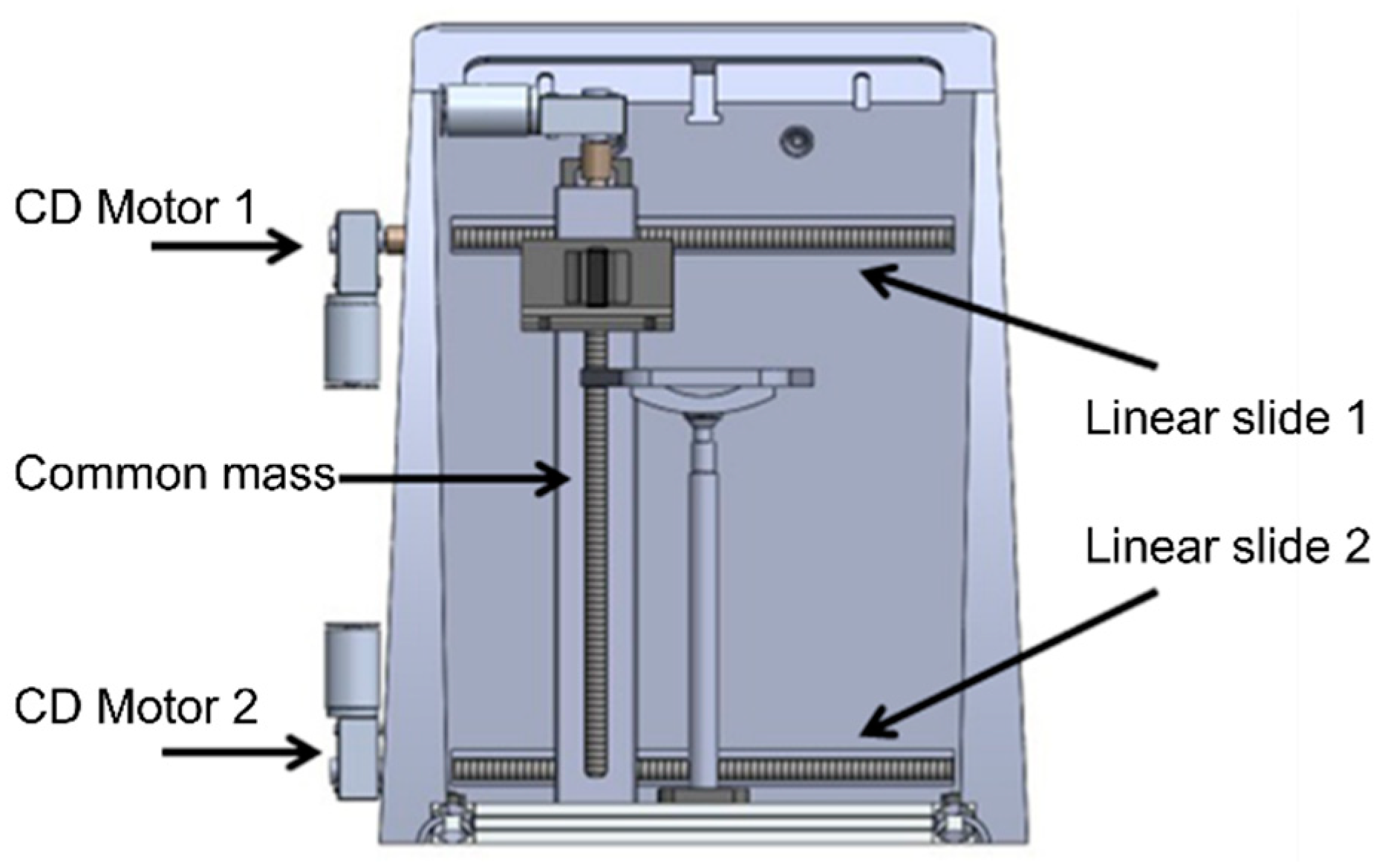
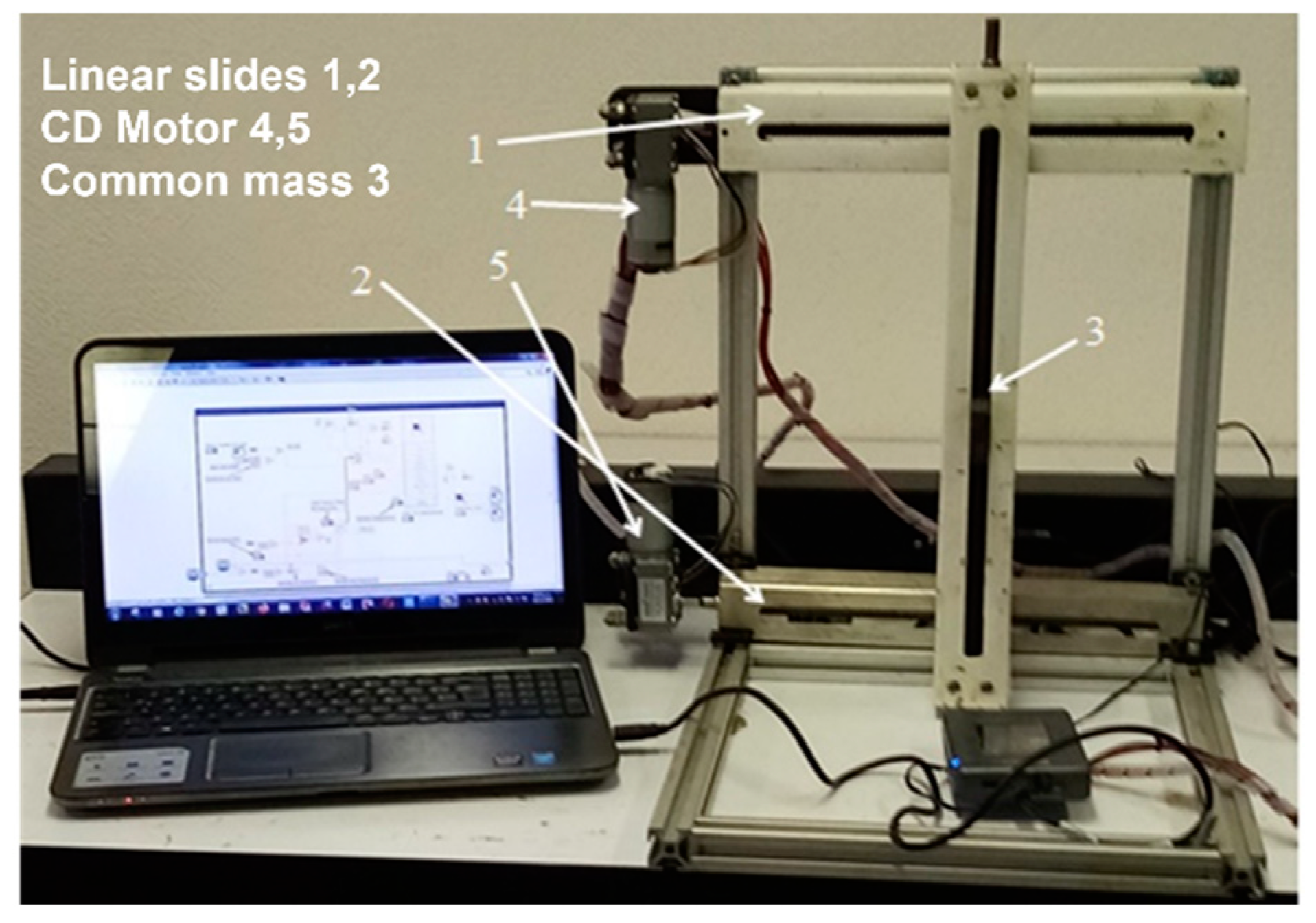
2. Materials and Methods

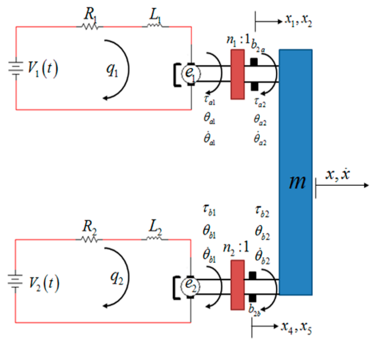
2.1. Mathematical Model

The problem addressed in this article is part of a 2 degree of freedom (DOF) ankle rehabilitation system [20]. For the movement in the x axis, it is proposed to use 2 motors to move the mass, through the use of linear slides (screw and nut).
Next, a dynamic model is proposed for the two linear slides coupled to the same mass, see Figure 1. In mathematical modeling, only viscous damping ( b 2 i ) is considered and friction between components is neglected. The control objective is to smoothly move the mass, with the actuators, at the same position and speed.
The System shown in Figure 1 is represented in a schematic diagram in Figure 2. The parameters and variables of the DC motor are shown, as well as the coupling by means of two linear guides with screws, to convert rotational to translational movement.
Based on Figure 2, the dynamic model of the linear slides coupled to the same mass is obtained using the Euler-Lagrange equations as follows [21]:
L i d i i d t + R i i i = V i k b i n i p i x ˙
I i p i + m p i x ¨ + b 2 i p i x ˙ = n i k f i i i
Table 1 shows the description of the parameters and variables of the dynamic model.
In this problem, it is considered that the displacements of each linear guide are different, so a different displacement variable ( y 1 , z 1 ) is used for each linear slide.
Using the variables and parameters (Table 1) in Equations (1) and (2), the following dynamic model is obtained for the two sliders
L 1 d i 1 d t + R 1 i 1 = V 1 k b 1 n 1 p 1 y ˙ 1
I 1 p 1 + m p 1 y ¨ 1 + b 21 p 1 y ˙ 1 = n 1 k f 1 i 1
L 2 d i 2 d t + R 2 i 2 = V 2 k b 2 n 2 p 2 z ˙ 1
I 2 p 2 + m p 2 z ¨ 1 + b 22 p 2 z ˙ 1 = n 2 k f 2 i 2
The mathematical model turns out to be of sixth order. From Equations (4) and (6), we solve for i 1 and i 2 , and differentiating with respect to time, we calculate d i 1 d t and d i 2 d t . Subsequently, substituting these variables in Equations (3) and (5) and making the respective variable changes, α 1 = I 1 p 1 + m p 1 ; α 2 = I 2 p 2 + m p 2 , the model is as follows
y 1 3 = n 1 k f 1 α 1 L 1 V 1 b 21 α 1 p 1 + R 1 L 1 y ¨ 1 n 1 2 k f 1 k b 1 α 1 L 1 p 1 + R 1 b 21 α 1 L 1 p 1 y ˙ 1
z 1 3 = n 2 k f 2 α 2 L 2 V 2 b 22 α 2 p 2 + R 2 L 2 z ¨ 1 n 2 2 k f 2 k b 2 α 2 L 2 p 2 + R 2 b 22 α 2 L 2 p 2 z ˙ 1
It is observed that the linear model given in Equations (7) and (8) is a MIMO system with two control inputs and two outputs of interest to regulate. These equations correspond to each displacement of each linear slide; the control input is the voltage and the output is the displacement.
Now, representing the system in state variables in its typical linear form, we have the following:
y ˙ 1 = x 2 x ˙ 2 = x 3 x ˙ 3 = n 1 k f 1 α 1 L 1 u 1 b 21 α 1 p 1 + R 1 L 1 x 3 n 1 2 k f 1 k b 1 α 1 L 1 p 1 + R 1 b 21 α 1 L 1 p 1 x 2 z ˙ 1 = x 5 x ˙ 5 = x 6 x ˙ 6 = n 2 k f 2 α 2 L 2 u 2 b 22 α 2 p 2 + R 2 L 2 x 6 n 2 2 k f 2 k b 2 α 2 L 2 p 2 + R 2 b 22 α 2 L 2 p 2 x 5
Considering the multivariable linear system Equation (9) as: x ˙ = A x + B u , y = C x where the state vector is defined as: x = x 1   x 2   x 3   x 4   x 5   x 6 T R 6 and u = u 1   u 2 T R 2 , being the matrix A as:
A = 0 1 0 0 0 a 0 0 1 0 b 0 0 0 0 0 0 0 0 0 0 0 0 0 0 0 0 0 0 0 1 0 0 1 c d
where
a = n 1 2 k f 1 k b 1 α 1 L 1 p 1 + R 1 b 21 α 1 L 1 p 1 ,   b = b 21 α 1 p 1 + R 1 L 1 c = n 2 2 k f 2 k b 2 α 2 L 2 p 2 + R 2 b 22 α 2 L 2 p 2 ,   d = b 22 α 2 p 2 + R 1 L 1
and matrix B is defined as:
B = 0 0 0 0 n 1 k f 1 α 1 L 1 0                 0 0                 0 0                 0 n 2 k f 2 α 2 L 2
Being the matrix B of rank 2 and is constituted by the column vectors B = b 1   b 2 .

2.2. Differential Parameterization of the Dynamic Model

This section deals with the differential flatness property of the linear dynamical system given by Equation (9). A linear dynamic system is differentially flat if and only if it is controllable [22]. In order to check that the MIMO dynamic system given in Equation (9) is controllable, it must satisfy that the Kalman controllability matrix is full rank. Said matrix in its general form is given as:
K C = b 1 , , A γ 1 1 b 1 , b 2 , , A γ 2 1 b 1 , b 2 , , A γ m 1 b m
with γ i ,   i = 1 , , m , being the Kronecker controllability indices of the system, which obviously satisfy the following expression i γ i = n r . Where n r is the range of the system.
The flat outputs of the linear MIMO system given in Equation (9) are calculated through the following expression:
F = ϕ i ϕ m C 1 x
with ϕ i ,   i = 1 , , m being an n-dimensional row vector of the form:
ϕ j = 0 , , 1 λ t h , , 0
with the 1 in the i = 1 j λ i -th position.
Therefore, the controllability matrix of the system is given by:
K C = B , A B , A 2 B , A 3 B , A 4 B , A 5 B
Substituting the corresponding values in the matrix Equation (15), the matrix KC is calculated, which results in a full rank matrix. Therefore, it is concluded that the linear system is controllable and, therefore, differentially flat.
The calculation of the flat outlets is carried out with the help of the following definition:
Given matrix A and columns b1 and b2 of matrix B such that B = b 1 , b 2 , the following full rank matrix C R 2 x 6 is calculated, whose columns belong to the Kalman controllability matrix.
C = b 1 , A b 1 , A 2 b 1 , b 2 , A b 2 , A 2 b 2
The columns of matrix C are selected from K C R 6 x 12 from the selection of the Kronecker indices, where λ1 = 3 and λ2 = 3. Using Equation (12), the flat outputs are calculated as follows
F 0 0 1 0 0 0 0 0 0 0 0 1 C 1 x
The flat outputs of the system turn out to be F 1 = x 1 and F 2 = x 4 ; in the case of this system, the flat outputs have a physical interpretation, these being the angular positions of both actuators. Expressing Equation (9) in terms of the flat outputs and their successive derivatives, the differential parameterization of the dynamic model is defined by:
x 1 = F 1 F 1 3 = n 1 k f 1 α 1 L 1 u 1 n 1 2 k f 1 k b 1 α 1 L 1 p 1 + R 1 b 21 α 1 L 1 p 1 F ¨ 1 b 21 α 1 p 1 + R 1 L 1 F ˙ 1 x 4 = F 2 F 2 3 = n 2 k f 2 α 2 L 2 u 2 n 2 2 k f 2 k b 2 α 2 L 2 p 2 + R 2 b 22 α 2 L 2 p 2 F ¨ 2 b 22 α 2 p 2 + R 2 L 2 F ˙ 2

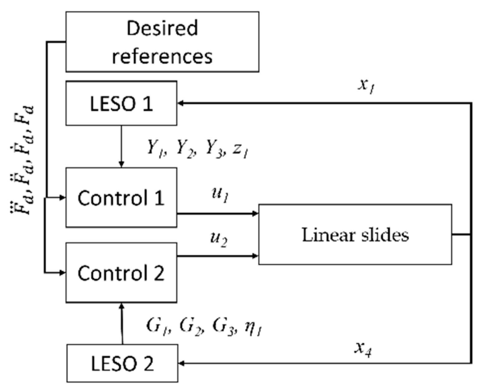
2.3. Active Disturbance Rejection Control (ADRC)

In this section, the position control for the system of the two linear slides is designed; this multivariable controller is based on the active disturbance rejection technique. From Equation (18), the control inputs are solved and the highest order derivatives are replaced by auxiliary variables v a u x 1 and v a u x 2 , giving the following expression:
u 1 u 2 = α 1 L 1 n 1 k f 1 0 0 α 2 L 2 n 2 k f 2 v a u x 1 v a u x 2 + Φ 1 Φ 2
F 1 3 = v a u x 1 , F 2 3 = v a u x 2
Φ 1 = n 1 2 k f 1 k b 1 α 1 L 1 p 1 + R 1 b 21 α 1 L 1 p 1 F ¨ 1 + b 21 α 1 L 1 p 1 + R 1 L 1 F ˙ 1
Φ 2 = n 2 2 k f 2 k b 2 α 2 L 2 p 2 + R 2 b 22 α 2 L 2 p 2 F ¨ 2 + b 22 α 2 p 2 + R 2 L 2 F ˙ 2
The functions Φ 1 and Φ 2 represent the endogenous and exogenous perturbations of the system, which are assumed unknown, but bounded. These functions are estimated by means of two Extended State Observers (ESO’s), which are calculated using the following expression:
F 1 3 F 2 3 = α 1 L 1 n 1 k f 1 0 0 α 2 L 2 n 2 k f 2 1 u 1 u 2 Φ 1 Φ 2
For the design of extended state linear observers, the following considerations are assumed:
  • The flat outputs F 1 and F 2   are measured;
  • The nominal values of the system parameters are known;
  • The control inputs are u 1 and u 2 are available;
  • The disturbance functions Φ 1 and Φ 2 are unknown but considered as bounded;
  • The estimated variables of the disturbance functions will be denoted as z 1 and η 1 .
Subsequently, the estimated variables of the flat outputs and their successive derivatives are denoted by:
Y 1 = F ^ 1 ; d F ^ 1 d t = Y 2 ; d 2 F ^ 1 d t 2 = Y 3 ; G 1 = F ^ 2 ; d F ^ 2 d t = G 2 ; d 2 F ^ 2 d t 2 = G 3
From Equation (23), the linear extended state observers given in (LESO 1) Equation (25) and (LESO 2) Equation (26) are designed [14,23]:
d d t Y 1 = Y 2 + λ 5 F 1 Y 1 d d t Y 2 = Y 3 + λ 4 F 1 Y 1 d d t Y 3 = n 1 k f 1 α 1 L 1 u 1 + z 1 + λ 3 F 1 Y 1 z ˙ 1 = z 2 + λ 2 F 1 Y 1 z ˙ 2 = z 3 + λ 1 F 1 Y 1 z ˙ 3 = λ 0 F 1 Y 1
d d t G 1 = G 2 + λ 5 F 2 G 1 d d t G 2 = G 3 + λ 4 F 2 G 1 d d t G 3 = n 2 k f 2 α 2 L 2 u 2 + η 1 + λ 3 F 2 G 1 η ˙ 1 = η 2 + λ 2 F 2 G 1 η ˙ 2 = η 3 + λ 1 F 2 G 1 η ˙ 3 = λ 0 F 2 G 1
The coefficients λ 5 , λ 4 , λ 3 , λ 2 , λ 1 , λ 0 of the observers are constant and selected by means of a sixth order Hurwitz polynomial. On the other hand, the design of the position controllers by active disturbance rejection is carried out from Equation (19), and these are given by:
u 1 = α 1 L 1 n 1 k f 1 v a u x 1
u 2 = α 2 L 2 n 2 k f 2 v a u x 2
The desired dynamics imposed by the auxiliary variables v a u x 1 and v a u x 2 , and by the adaptation of the values estimated by the extended state observers are
v a u x 1 = F 1 d 3 k 2 Y 3 F ¨ 1 d k 1 Y 2 F ˙ 1 d k 0 Y 1 F 1 d z 1
v a u x 2 = F 2 d 3 k 2 G 3 F ¨ 2 d k 1 G 2 F ˙ 2 d k 0 G 1 F 2 d η 1
where the coefficients k 2 , k 1 , k 0 are constant and selected such that the closed-loop third-order characteristic polynomial is Hurwitz and the variables F 1 d 3 , F ¨ 1 d , F ˙ 1 d , F 1 d and F 2 d 3 , F ¨ 2 d , F ˙ 2 d , F 2 d   are the desired reference variables constructed using a tenth-order Bézier polynomial.

2.4. Desired Reference Trajectory

The ankle rehabilitation machine must guarantee safe rehabilitation movements. Given that, the movements must be smooth and continuous. The desired reference trajectories are given by the following tenth-order Bezier polynomial.
x 1 d t = 0 x 10 x 1 f           0 t < t i t i t < t f t > t f
x 10 = x i 0 + x i f x i 0 a 0 a 1 μ + a 2 μ 2 a 3 μ 3 + a 4 μ 4 a 5 μ 5 μ = t t i t f t i
where x i 0 = x 1 d t i is the initial desired position and x i f = x 1 d t f is the final desired position. The parameters of the Bezier polynomial were selected as: a0 = 252, a1 = 1050, a2 = 1800, a3 = 1575, a4 = 700 and a5 = 126.

2.5. System Stability Analysis ESO-ADRC

From Equations (25) and (26), the test of the dynamic error of the output of the extended state observers is verified. Setting the output estimation error as follows
e o = F i F ^ i
where i = {1,2}. The first derivative of e o , for the flat output F 1 , is given by:
d e o d t = F ˙ 1 d F ^ 1 d t = F ˙ 1 Y 2 λ 5 e o e ˙ o + λ 5 e o = F ˙ 1 Y 2
Finding the time derivative of Equation (33)
e ¨ o + λ 5 e ˙ o = F ¨ 1 d Y 2 d t = F ¨ 1 Y 3 λ 4 e o
The third time derivative of e o is
e o + λ 5 e ¨ o + λ 4 e ˙ o + λ 3 e o = F 1 d Y 3 d t = Φ 1 z 1
The fourth time derivative of e o , is obtained by
e o 4 + λ 5 e o + λ 4 e ¨ o + λ 3 e ˙ o = Φ ˙ 1 z ˙ 1 e o 4 + λ 5 e o + λ 4 e ¨ o + λ 3 e ˙ o + λ 2 e o = Φ ˙ 1 z 2
The fifth time derivative of e o can be expressed by
e o 5 + λ 5 e o 4 + λ 4 e o + λ 3 e ¨ o + λ 2 e ˙ o + λ 1 e o = Φ ¨ 1 z 3
The sixth time derivative of e o is the dynamics of the estimation error and is given by
e o 6 + λ 5 e o 5 + λ 4 e o 4 + λ 3 e 0 + λ 2 e ¨ o + λ 1 e ˙ o + λ 0 e o = Φ 1
It is concluded that the unperturbed version ( Φ 1 ( t ) = 0 ) of the observation error dynamics can be specified to become asymtotically exponentially stable through the choice of suitable Hurwitz design coefficients:
P d o b s s = s 2 + 2 ξ ω o s + ω o 2 3
Hence,
λ 5 = 6 ξ ω o ; λ 4 = 12 ξ 2 + 3 ω o 2 ; λ 3 = 8 ξ 2 + 12 ξ ω o 3 ; λ 2 = 12 ξ 2 + 3 ω o 4 ; λ 1 = 6 ξ ω o 5 ; λ 0 = ω o 6
For the flat output F 2 , the same procedure applies.
Let Φ 1 s denote the Laplace transform of the disturbance signal Φ 1 t . The estimation error dynamics is described by the perturbed band-pass stable filter,
E ˜ 0 s = s 3 Φ 1 s s 6 + λ 5 s 5 + λ 4 s 4 + λ 3 s 3 + λ 2 s 2 + λ 1 s + λ 0
which enjoys infinite attenuation at very low, and at very high frequencies [23].
Finally, applying the final value theorem [24] to Equation (40):
lim t e ˜ 0 t = lim s 0 s E ˜ 0 s = 0

3. Results

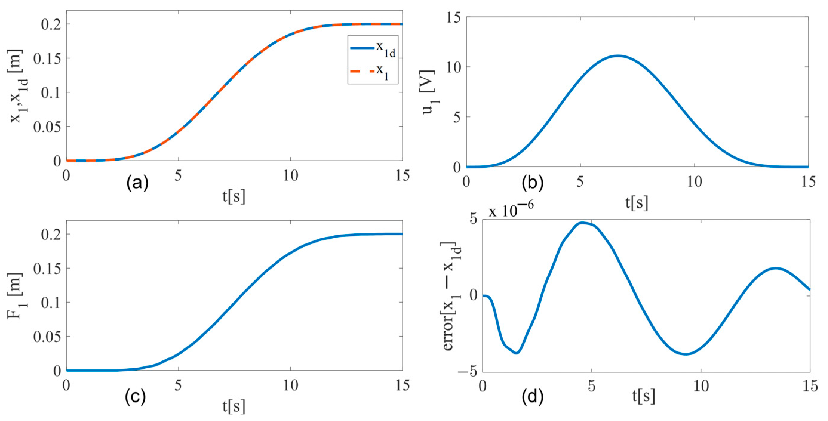
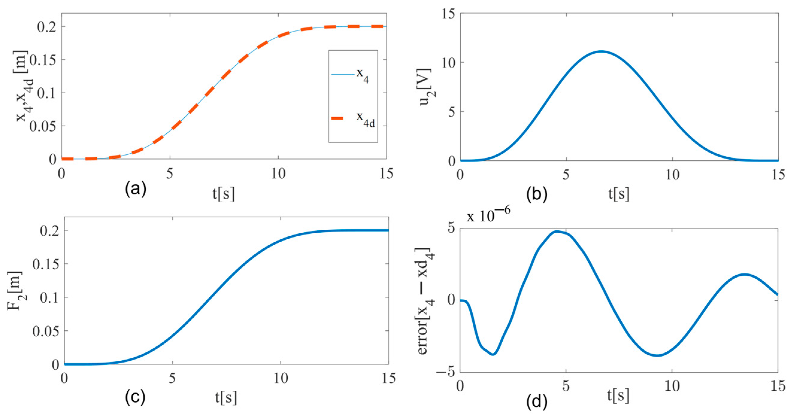
3.1. Simulation Results

Using the Matlab-Simulink environment, simulation results of the multivariable active disturbance rejection control system in closed loop were obtained. The simulation consisted of implementing the two controllers, Equations (27) and (28), as well as the extended state observers, (LESO 1) Equation (25) and (LESO 2) Equation (26). Figure 3 shows the block diagram of the implemented control scheme.
Figure 4a shows the response of the linear position x 1 , as well as the desired reference position x 1 d . The desired trajectory, Bezier polynomial, starts from the rest position ( x 1 d = 0   m ), and in 15 s it reaches the final position ( x 1 d = 0.2   m ). Similarly, in the desired path for the second linear guide. Figure 4b shows the response of the control input u 1 which does not exceed the nominal voltage limit of +12 V, while Figure 4c shows the estimation of the first flat output F 1 and Figure 4d shows the response of the error of linear position x 1 x 1 d corresponding to the first slider, which is about 4.5 × 10 6 peak amplitude. It can be seen that the control u 1 (voltage) is applied smoothly to follow the desired trajectory, increasing until reaching the maximum value (12 V) for the midpoint of the trajectory, to subsequently decrease the voltage and, thus, decelerate and reach smoothly to the desired position value.
Figure 5a shows the response of the linear position x 4 , as well as the desired reference position x 4 d . Figure 5b shows the response of control input u 2 which does not exceed the nominal voltage level +12 V, and with a behavior similar to the control u 1 . Figure 5c shows the estimate of the second flat output F 2 . Figure 5d shows the response of the position error x 4 x 4 d , which has an approximate peak value of 4.5 × 10 6   m .

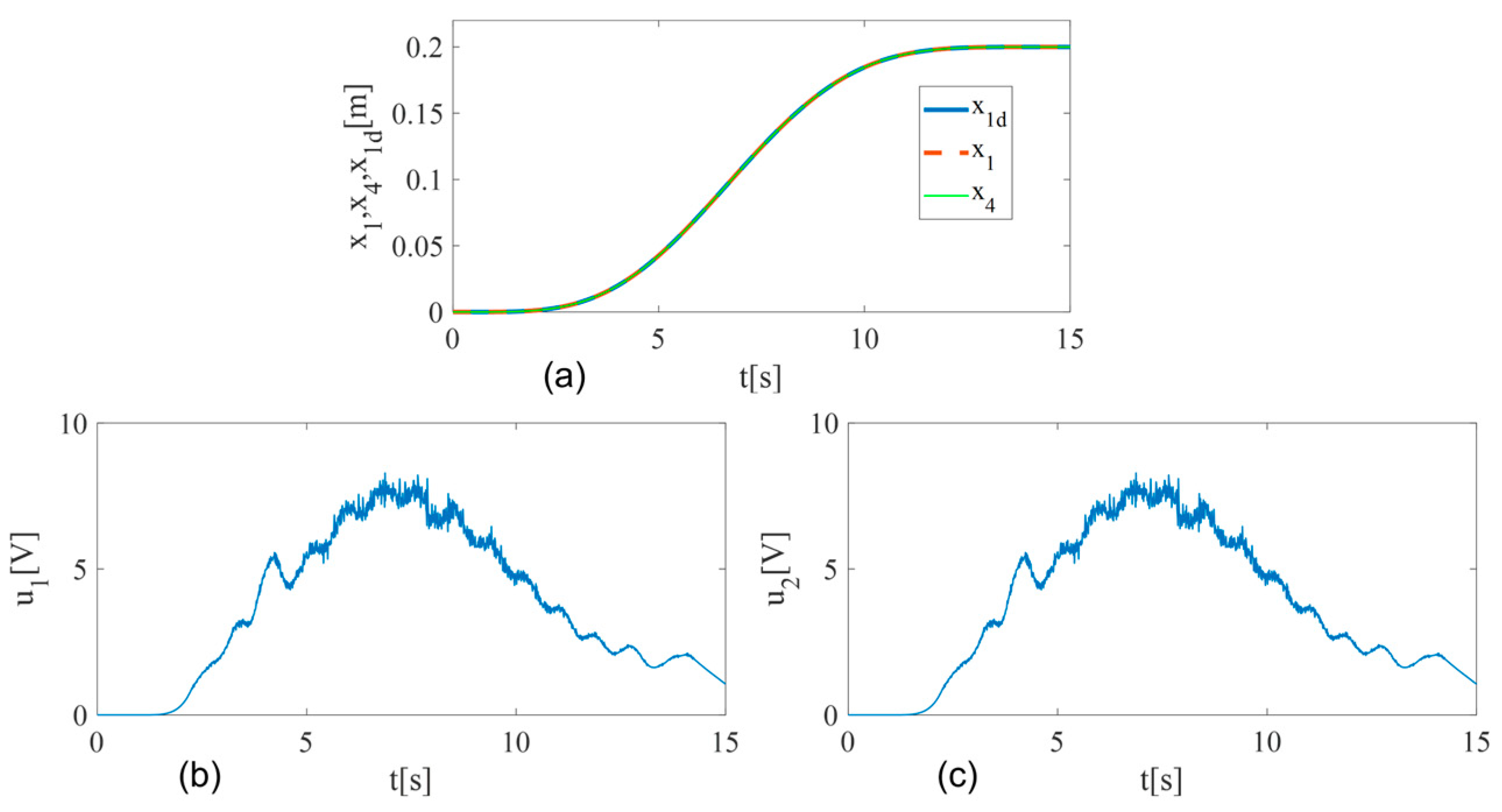
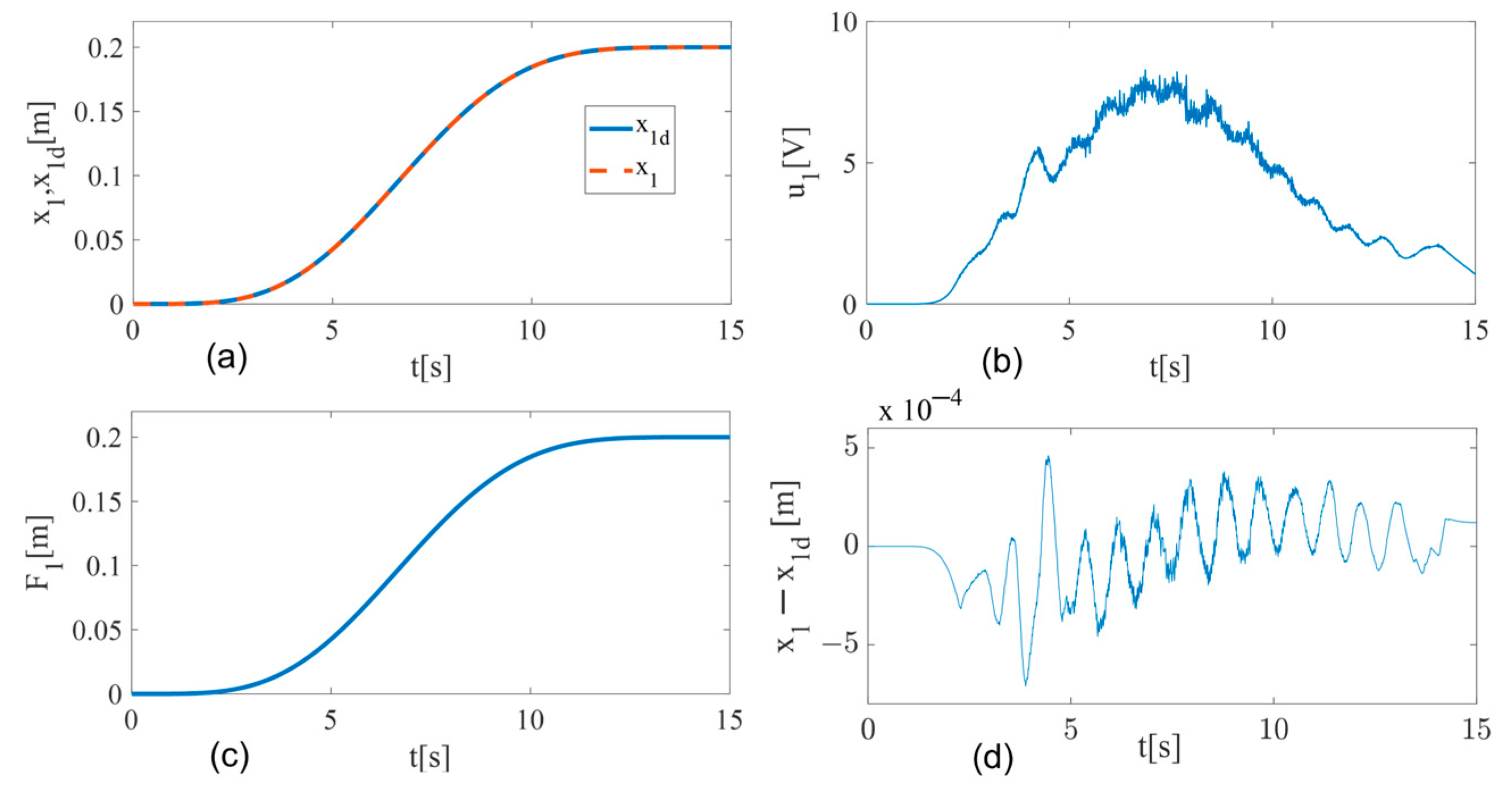
3.2. Experimental Results

The experimental results obtained from the closed-loop system platform show the advantages of using this control technique. The first one is that the control law does not require knowledge of all the plant parameters; secondly, it is only required to measure the flat outputs of the system. Third, it actively estimates unknown internal and external disturbances. This information is fed back to the controller to reduce its effects on the plant. Fourth, it synchronizes the positions and speeds of the actuators from the initial displacement. Fifth, the torque demand produced by the two actuators is equal.
Figure 6 shows the experimental platform. You can see the two horizontal linear sliders that use endless screws to produce the displacement of the common mass. The two 12 V DC geared motors (construction: Permanent Magnet), with Magnetic Hall encoder, drive the sliders. Also seen is the National Instruments MY-RIO board, which is programmed in the LabView environment. Therefore, the controllers and observers for the motors are programmed in LabView. In addition, the viscous friction component in each of the sliders was modified, with the intention of causing a difference in parametric uncertainty in the platform.
Figure 7a shows the two responses of the linear position of the sliders, where the linear position of the second slider has a slight delay with respect to the desired reference; however, in the final time programmed in the reference, the two positions of each slider reach the reference at the same time. It is worth mentioning that in the path of the two responses x 1 x 4 , which represents a challenge for the controller (ADRC) to synchronize the positions and speeds of both actuators. Figure 7b,c show the control input responses u 1 and u 2 , which are physically the forces for both sliders that smoothly slide the same mass. There is a difference between them before reaching 5 s, since the first slider presents a different viscous friction in sliding.
Extended State Observers (ESO’s) estimate internal and external disturbances to later reduce them using the multivariable controller; this can be observed in the responses shown in Figure 8 and Figure 9.
Figure 8a shows the position tracking response x 1 together with its desired trajectory reference x 1 d . Figure 8b shows the response of the control input of motor 1, u 1 , and Figure 8c shows the observed variable, F 1 ; finally, Figure 8d shows the response of the actual position error minus the desired position, x 1 x 1 d ; the value of the maximum error is 5 × 10 4   m , so it can be considered an acceptable error.
Figure 9a shows the tracking of the desired trajectory, x 4 d , together with the real trajectory, x 4 ; Figure 9b shows the control input of motor 2, u 2 , and Figure 9c shows the observed variable, F 2 ; Figure 9d shows the actual position error minus the desired position, x 4 x 4 d . The value of the maximum error is 5 × 10 4   m , so it can also be considered an acceptable error.
The input signals of the controllers with active disturbance rejection (ADRC), u 1 and u 2 , can be seen in Figure 8 and Figure 9, which do not exceed 12 Volts.
During the experimental tests with the physical linear guides, Figure 6, the common mass was made to move a distance of 0.2 m, verifying the robustness and advantages that ADCR is capable of when coinciding with minimum error, the actual and desired trajectories. It was also possible to graph the signal delivered by the extended state linear observers, (LESO’s), F 1 and F 2 , as can be seen in Figure 8c and Figure 9c.

4. Discussion

The ADRC based on extended state linear observers, implemented in this multivariable electromechanical system for smooth trajectory tracking, estimates the factors that affect the plant, including nonlinear dynamics, uncertainties, mismatches and external disturbances due to viscous friction differences that can occur on each linear guide.
Based on the simulation and experimental results, a good performance of the controller can be observed in the synchronization of the angular positions of the two actuators, to finally make the linear displacement smoothly follow the desired trajectory of the mass coupled in common, having a maximum error of 5 × 10 4   m .

5. Conclusions

The combination of Extended State Linear Observers (ESO’s) with the Active Disturbance Rejection Control (ADRC) technique achieves a robust cooperative control system in the face of parametric and external disturbances that occur in the system. Therefore, in this particular case, it has been achieved that the two actuators (DC motors) can be coupled during the displacement of the common mass, making each of the linear guides have an equal advance, that is, x 1 = x 4 . This eliminates the possibility that when the two linear guides move unequally, they produce undesirable torque on the table that supports the common mass, causing significant damage to the system. Both the simulations and the tests carried out verify the effectiveness of the controllers as well as that of the observers.

Author Contributions

Conceptualization, A.B.O., F.A.G.B. and J.V.T.; methodology, J.V.T., H.M.B.A. and A.B.O.; software, F.A.G.B., E.S.B. and M.C.R.; validation, J.S.V.M. and E.S.B.; formal analysis, F.A.G.B., A.B.O. and M.C.R.; investigation, M.C.R., H.M.B.A., J.V.T. and J.S.V.M.; resources, J.V.T., H.M.B.A. and E.S.B.; data curation, F.A.G.B.; writing—original draft preparation, E.S.B., M.C.R. and J.S.V.M.; writing—review and editing, M.C.R.; visualization, J.S.V.M.; supervision, A.B.O. and F.A.G.B.; project administration, F.A.G.B. and J.V.T.; funding acquisition, J.S.V.M., J.V.T. and H.M.B.A. All authors have read and agreed to the published version of the manuscript.

Funding

This research received no external funding.

Institutional Review Board Statement

Not applicable.

Informed Consent Statement

Not applicable.

Data Availability Statement

Not applicable.

Conflicts of Interest

The authors declare no conflict of interest.

References

  1. Linares-Flores, J.; Reger, J.; Sira-Ramírez, H. Sensorless tracking control of two DC-drives via a double Buck-converter. In Proceedings of the 45th IEEE Conference on Decision and Control, San Diego, CA, USA, 13–15 December 2006. [Google Scholar]
  2. Sira-Ramírez, H.; Linares-Flores, J.; García-Rodríguez, C.; Contreras-Ordaz, M.A. On the control of the permanent magnet synchronous motor: An active disturbance rejection control approach. IEEE Trans. Control. Syst. Technol. 2014, 22, 2056–2063. [Google Scholar] [CrossRef]
  3. Linares-Flores, J.; Guerrero-Castellanos, J.F.; Lescas-Hernández, R.; Hernández-Méndez, A.; Vázquez-Perales, R. Angular speed control of an induction motor via a solar powered boost converter-voltage source inverter combination. Energy 2019, 166, 326–334. [Google Scholar] [CrossRef]
  4. Sira-Ramırez, H.; Linares-Flores, J.; Luviano-Juarez, A.; Cortes-Romero, J. Ultramodelos Globales y el Control por Rechazo Activo de Perturbaciones en Sistemas No lineales Diferencialmente Planos. Rev. Iberoam. Autom. Inform. Ind. 2015, 12, 133–144. [Google Scholar] [CrossRef]
  5. Ramírez-Neria, M.; Sira-Ramírez, H.; Garrido-Moctezuma, R.; Luviano-Juarez, A. Linear active disturbance rejection control of underactuated systems: The case of the Furuta pendulum. ISA Trans. 2014, 53, 920–928. [Google Scholar] [CrossRef] [PubMed]
  6. Guerrero-Ramírez, E.; Martínez-Barbosa, A.; Guzmán-Ramírez, E.; Linares-Flores, J.; Sira-Ramírez, H. Control del Convertidor CD/CD Reductor–Paralelo Implementado en FPGA. Rev. Iberoam. Autom. Inform. Ind. 2018, 15, 309–316. [Google Scholar] [CrossRef]
  7. Tian, L.; Li, D.; Huang, C.E. Decentralized controller design based on 3-order active-disturbance-rejection-control. In Proceedings of the 10th World Congress on Intelligent Control and Automation, Beijing, China, 6–8 July 2012; pp. 2746–2751. [Google Scholar] [CrossRef]
  8. Sira-Ramirez, H.; Luviano-Juarez, A.; Cortes-Romero, J. Control lineal robusto de sistemas no lineales diferencialmente planos. Rev. Iberoam. Autom. Inform. Ind. 2011, 8, 14–28. [Google Scholar] [CrossRef]
  9. Sun, L.; Dong, J.; Li, D.; Lee, K.Y. A practical multivariable control approach based on inverted decoupling and decentralized active disturbance rejection control. Ind. Eng. Chem. Res. 2016, 55, 2008–2019. [Google Scholar] [CrossRef]
  10. Chang, X.; Li, Y.; Zhang, W.; Wang, N.; Xue, W. Active disturbance rejection control for a flywheel energy storage system. IEEE Trans. Ind. Electron. 2014, 62, 991–1001. [Google Scholar] [CrossRef]
  11. Xia, Y.; Chen, R.; Pu, F.; Dai, L. Active disturbance rejection control for drag tracking in mars entry guidance. Adv. Space Res. 2013, 53, 853–861. [Google Scholar] [CrossRef]
  12. Sira-Ramírez, H.; Rosales-Díaz, D. Decentralized active disturbance rejection control of power converters serving a time varying load. In Proceedings of the 33rd Chinese Control Conference, Nanjing, China, 22–24 May 2014; pp. 4348–4353. [Google Scholar] [CrossRef]
  13. Ramírez-Neria, M.; Madonski, R.; Luviano-Juárez, A.; Gao, Z.; Sira-Ramírez, H. Design of ADRC for Second-Order Mechanical Systems without Time-Derivatives in the Tracking Controller. In Proceedings of the 2020 American Control Conference (ACC), Denver, CO, USA, 1–3 July 2020; pp. 2623–2628. [Google Scholar] [CrossRef]
  14. Linares-Flores, J.; Hernández-Méndez, A.; Guerrero-Castellanos, J.F.; Mino-Aguilar, G.; Espinosa-Maya, E.; Zurita-Bustamante, E.W. Decentralized ADR angular speed control for load sharing in servomechanisms. In Proceedings of the 2018 IEEE Power and Energy Conference at Illinois (PECI), Champaign, IL, USA, 22–23 February 2018; pp. 1–5. [Google Scholar] [CrossRef]
  15. Sun, L.; Li, D.; Hu, K.; Lee, K.Y.; Pan, F. On tuning and practical implementation of active disturbance rejection controller: A case study from a regenerative heater in a 1000 MW power plant. Ind. Eng. Chem. Res. 2016, 55, 6686–6695. [Google Scholar] [CrossRef]
  16. Barahona, J.L.; Juárez, J.A.; Galván, G.S.; Linares, J. Active disturbance rejection control of temperature of thermoelectric module. Rev. Iberoam. Autom. Inform. Ind. 2022, 19, 48–60. [Google Scholar] [CrossRef]
  17. Pulido-Flores, A.; Guerrero-Castellanos, J.F.; Linares-Flores, J.; Maya-Rueda, S.E.; Alvarez-Muñoz, J.U.; Escareno, J.; Mino-Aguilar, G. Active Disturbance Rejection Control for Attitude Stabilization of Multi-rotors UAVs with bounded inputs. In Proceedings of the 2018 International Conference on Unmanned Aircraft Systems (ICUAS), Dallas, TX, USA, 12–15 June 2018; p. 1181. [Google Scholar] [CrossRef]
  18. Guerrero-Castellanos, J.F.; Durand, S.; Muñoz-Hernández, G.A.; Marchand, N.; Romeo, L.L.G.; Linares-Flores, J.; Miño-Aguilar, G.; Guerrero-Sánchez, W.F. Bounded Attitude Control with Active Disturbance Rejection Capabilities for Multirotor UAVs. Appl. Sci. 2021, 11, 5960. [Google Scholar] [CrossRef]
  19. Xue, W.; Huang, Y. The active disturbance rejection control for a class of MIMO block lower-triangular system. In Proceedings of the 30th Chinese Control Conference, Yantai, China, 22–24 July 2011; pp. 6362–6367. [Google Scholar]
  20. Blanco Ortega, A.; Magadán Salazar, A.; Guzmán Valdivia, C.H.; Gómez Becerra, F.A.; Palacios Gallegos, M.J.; García Velarde, M.A.; Santana Camilo, J.A. CNC Machines for Rehabilitation: Ankle and Shoulder. Machines 2022, 10, 1055. [Google Scholar] [CrossRef]
  21. Gómez Becerra, F.A.; Olivares Peregrino, V.H.; Blanco Ortega, A.; Linares Flores, J. Optimal controller and controller based on differential flatness in a linear guide system: A performance comparison of indexes. Math. Probl. Eng. 2015, 2015, 589184. [Google Scholar] [CrossRef]
  22. Sira-Ramírez, H.; Agrawal, S. Differentially Flat Systems; Marcel Dekker: New York, NY, USA; Basel, Switzerland, 2004. [Google Scholar]
  23. Sira-Ramírez, H. From flatness, GPI observers, GPI control and flat filters to observer-based ADRC. Control. Theory Technol. 2018, 16, 249–260. [Google Scholar] [CrossRef]
  24. Shi, S.; Zeng, Z.; Zhao, C.; Guo, L.; Chen, P. Improved Active Disturbance Rejection Control (ADRC) with Extended State Filters. Energies 2022, 15, 5799. [Google Scholar] [CrossRef]
Figure 1. System with two linear slides.
Machines 11 00889 g001
Figure 2. Electrical-mechanical diagram of the linear slide system.
Machines 11 00889 g002
Figure 3. Block diagram for simulation in Matlab-Simulink.
Machines 11 00889 g003
Figure 4. Simulation results: first flat output responses. (a) Real and desired trajectories, x 1 and x 1 d , (b) Control input u 1 , (c) Observed variable F 1 , (d) Error x 1 x 1 d .
Machines 11 00889 g004
Figure 5. Simulation results: second flat output responses. (a) Real and desired trajectories, x 4 and x 4 d , (b) Control input u 2 , (c) Observed variable F 2 , (d) Error x 4 x 4 d .
Machines 11 00889 g005
Figure 6. Experimental platform of the two slides coupled to the same mass.
Machines 11 00889 g006
Figure 7. Experimental results of the two sliders: (a) x 1 , x 4 and x 1 d , (b) Control input u 1 for motor 1, (c) Control input u 2 for motor 2.
Machines 11 00889 g007
Figure 8. Experimental results of the sliders: (a) Real and desired trajectories, x 1 and x 1 d , (b) Control input u 1 , (c) Observed variable F 1 , (d) Error x 1 x 1 d .
Machines 11 00889 g008
Figure 9. Experimental results of the sliders: (a) Real and desired trajectories, x 4 and x 4 d , (b) Control input u 2 , (c) Observed variable F 2 , (d) Error x 4 x 4 d .
Machines 11 00889 g009
Table 1. System parameters.
VariableValueDescription
x -Mass displacement
m 10 kgMass
p 0.008 mScrew pitch
i (q)-Motor electrical current
k f 0.00706 Nm/AMotor torque coefficient
k b 0.00979 Vs/radMotor electrical coefficient
b 2 0.2 Ns/mViscous damping coefficient
L 0.00058 HArmature inductance
R 2.4 ΩArmature resistance
V VVoltage
n 0.027Speed ratio
I 14 × 10 7 kg m2Inertia moment
Disclaimer/Publisher’s Note: The statements, opinions and data contained in all publications are solely those of the individual author(s) and contributor(s) and not of MDPI and/or the editor(s). MDPI and/or the editor(s) disclaim responsibility for any injury to people or property resulting from any ideas, methods, instructions or products referred to in the content.

