Prediction of Stress and Deformation Caused by Magnetic Attraction Force in Modulation Elements in a Magnetically Geared Machine Using Subdomain Modeling

Abstract

This study presents an approach for calculating the stress and deformation increase in the modulation of magnetically geared machines using a mathematical method. An analytical method is employed to obtain the magnetic force density acting on the modulation components. Afterward, the proposed mathematical method predicts the mechanical characteristics. The 9 slots/32 poles/19 modulations model was evaluated via a comparison with the finite element method simulation.

1. Introduction

Currently, there are two approaches for addressing high-torque, low-speed applications. The first approach is a combination system of a gear and small-pole machine, which takes up more space. The second one entails using a large-pole-number machine that results in a complicated winding organization and increases the manufacturing cost. Both approaches have drawbacks. Hence, magnetically geared machines (MGMs) have become an increasingly attractive option for integrating permanent magnet synchronous machines (PMSMs) with magnetic gears into one structure. A comprehensive overview of the evolution and various approaches to MGMs has been presented [1,2,3]. Four different winding organizations for MGMs were investigated in [4,5], in which the authors proposed a dual-structure machine that improved the torque and reduced the cogging torque. To obtain the air gap flux density, an analytical method was employed [6]. Performance analyses of double-rotor or double-stator MGMs were also carried out in [7,8,9,10,11,12], where the authors presented a novel “pseudo” machine whose architecture is similar to a magnetic gear, in which the outer rotor has attached a winding having the same pole pair with the inner rotor. Using a spoke-type magnet [13,14,15] was an alternative to surface-type magnets [16] in the Vernier structure. Through changing the shape of the inner permanent magnet and the magnetization of the outer permanent magnet, a new structure has high torque density and high mechanical properties [17,18,19]. Combinations of spoke-type and Halbach-type rotors, as well as auxiliary teeth in the stator, were introduced [20,21]. A novel approach involving double-fed current is illustrated in [22,23,24,25], in which the authors introduced a novel bidirectional flux modulation concept, and [26] merged modulation and a stator into a single structure based on bidirectional concepts. To deepen comprehension and amplify output torque, investigations were carried out regarding gear ratios [27], parameter analysis [28], and optimization [29]. Notably, the eccentric harmonic magnetic gear was introduced in [30], proving particularly advantageous for applications demanding higher transmission ratios.

The aforementioned studies mainly focused on the electromagnetic aspect and superficially dealt with the mechanical analyses. In [31], the authors utilized FEM, which required several hours to obtain results. Ref. [32] experimentally verified a laminated structure in modulation after simulating a relevantly simplified model.

The FEM is widely recognized as a reliable solution for electrical machine analysis but has a significant running time when calculating problems. The subdomain analytical method, on the other hand, offers faster computational time and results that agree well with FEM simulations, making it a promising solution for MGM design and optimization. A comprehensive review can be found in the literature [33]. Two analytical methods are mainly used. The first one is based on the conformal mapping transformation method and a 2D relative permanence function [34]. The second method, which can be named subdomain modeling, is based on directly solving Maxwell’s equations and the boundary and interface conditions. Researchers have applied the subdomain method to various scenarios, such as radial-magnetization surface-mounted PMSM, Halbach array PMSM, coaxial magnetic gear, axial-field magnetic gear, and eccentricity effects in magnetic gear, as demonstrated in [35,36,37,38,39]. To consider iron parts with nonlinear cores, an enhanced 2D subdomain method in polar coordinates was explored [40,41].

The purpose of this paper is to present a 2D analytical model of a magnetic gear machine (MGM) based on the subdomain method. To the best of our knowledge, the analytical prediction of stress and deformation for a solid-structured modulation has not been explored previously. To address this gap, the authors utilized subdomain modeling to obtain the magnetic force density and proposed a purely mathematical approach for analyzing stress and deformation.

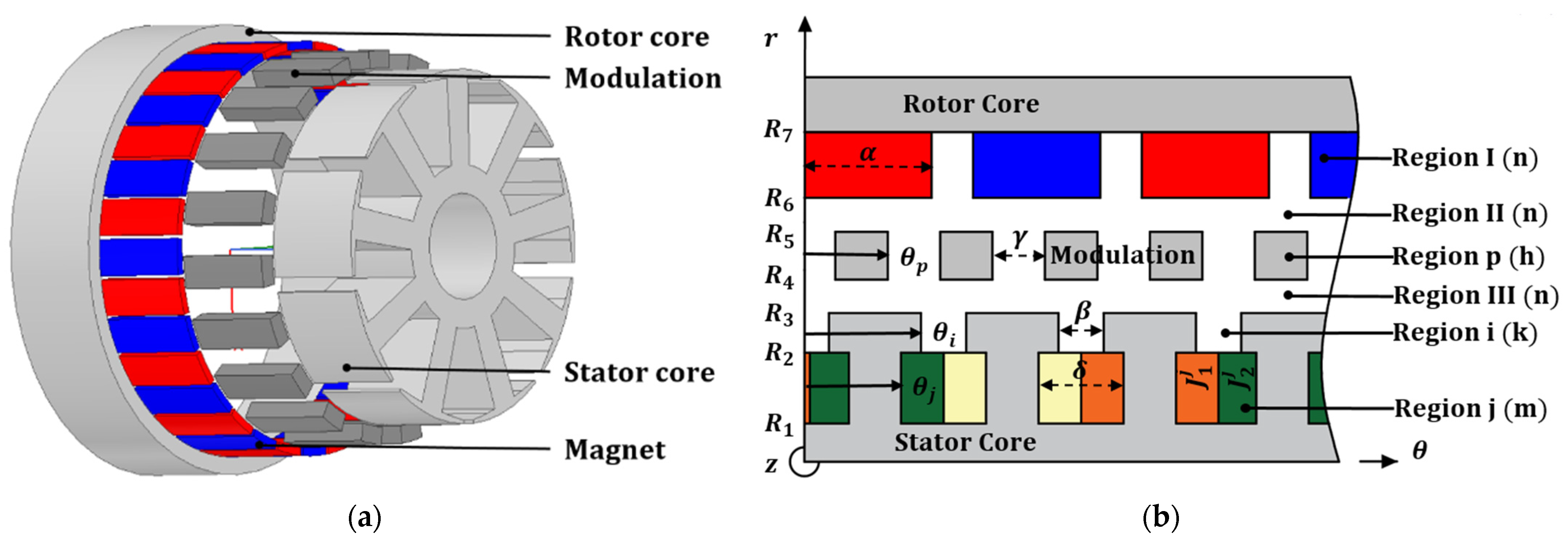
2. Magnetic Attraction Force

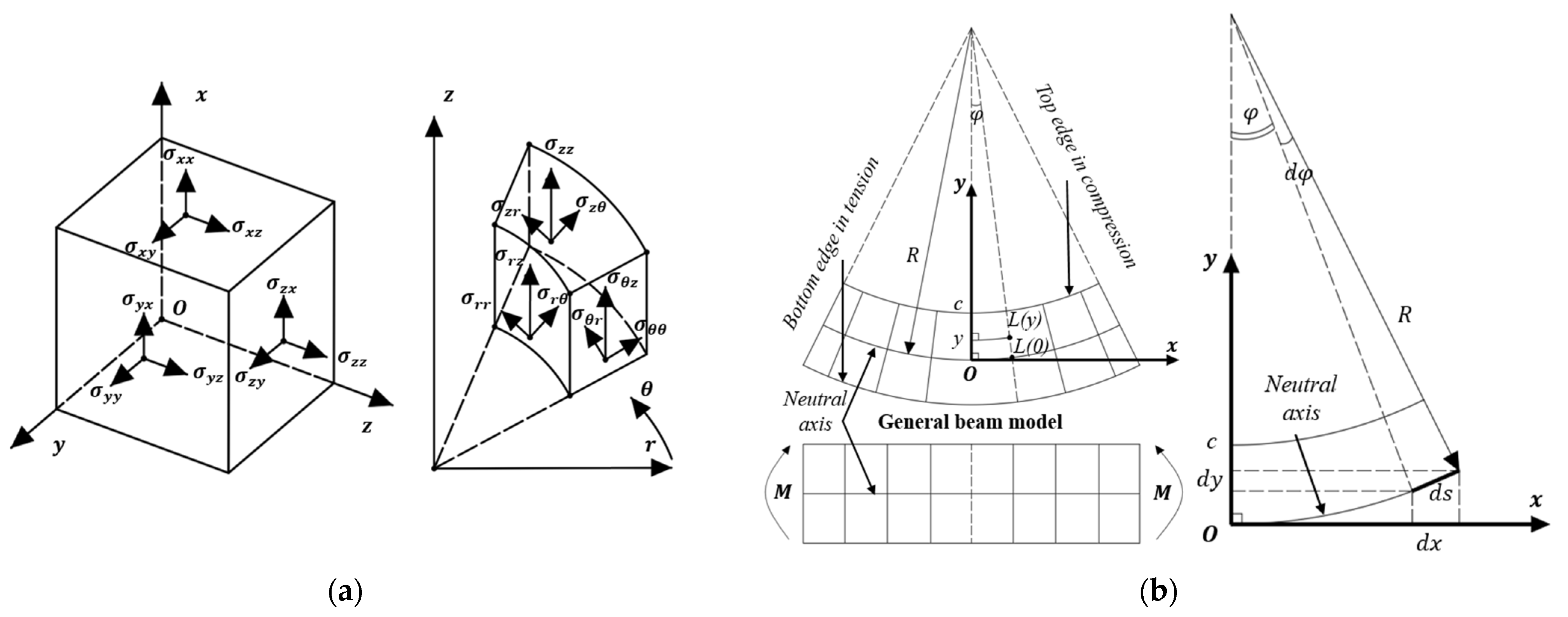
2.1. Governing Partial Differential Equations (PDEs)

Figure 1 presents an MGM model and its simplified reverent transfer model employed for the analytical method.

Table 1. The mechanical coefficients.

Parameters	Symbol	Unit	Value
Young’s modulus	$E$	${10}^5$ MPa	2
Shear ratio	$\kappa$	-	0.85
Bulk modulus	$G$	MPa	76,923

and

Table 2. Specification parameters.

Parameters	Symbol	Unit	Value
Outer magnet radius	$R_7$	mm	93.5
Inner magnet radius	$R_6$	mm	90.0
Outer modulation radius	$R_5$	mm	89.0
Inner modulation radius	$R_4$	mm	81.0
Outer stator radius	$R_3$	mm	80.0
Opening slot radius	$R_2$	mm	78.5
Slot radius	$R_1$	mm	37.0
Stack length	$L_{stk}$	mm	45.0
Magnet pitch ratio	$\alpha$	-	0.9
Modulation pitch	$\gamma$	$2\pi /P_m$ rad	0.5
Opening slot pitch	$\beta$	$2\pi /Q$ rad	0.125
Slot pitch	$\delta$	$2\pi /Q$ rad	0.8
Pole winding turn	-	-	56
Modulation number	$P_m$	-	19
Slot number	$Q$	-	9
Magnet pole pair	$Z_p$	-	16
Vacuum permeability	${\mu }_0$	$kg.m.s^{-2}.A^{-2}$	$4\pi {10}^{-7}$
Residual flux density of magnet	$B_0$	T	1.2
Magnetic magnetization of magnet	$M_0$	A/m	$B_0/{\mu }_0$

list the parameters of the machine and materials. Before solving the analytical solutions, the following assumptions are made:

• The end effects are ignored;
• The problem is two-dimensional in Cartesian coordinates;
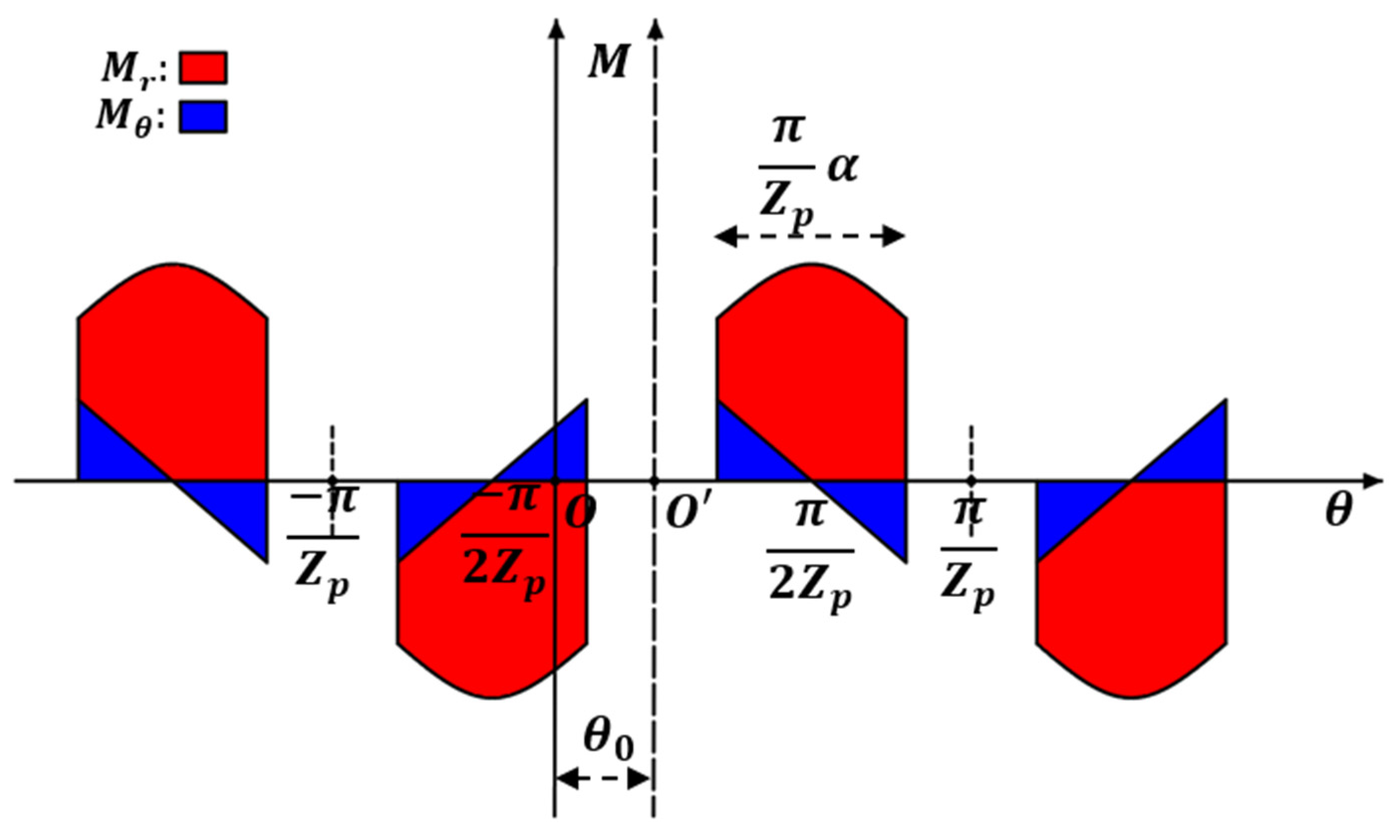
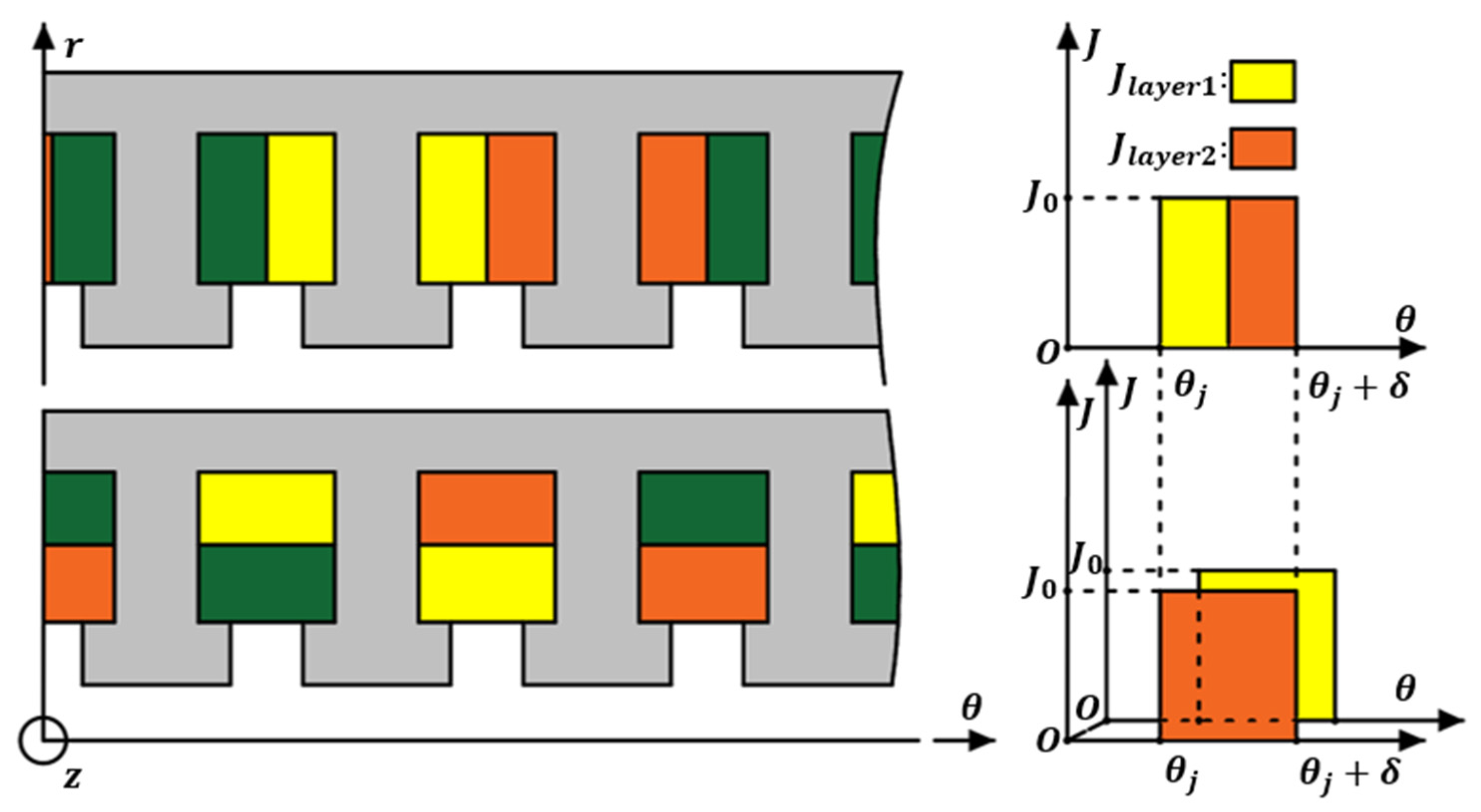
• Magnetic vector potential A, current density J, magnetization vector M, and magnetic flux density vector B, have the following non-zero components, respectively: A = [0, 0, A_z]; J = [0, 0, J_z]; M = [M_r, M_θ, 0]; B = [ B_r, B_θ, 0];
• The core materials have infinite permeability;
• The shaft is a non-magnetic material.

Through assuming 2D analysis in cylindrical coordinates, the governing partial differential equations (PDEs) for the six regions shown in Figure 1 are expressed as follows:

$$\frac{{\partial }^2{A}_z^I}{\partial r^2}+\frac{\partial A_z^I}{r\partial r}+\frac{{\partial }^2{A}_z^I}{r^2\partial {\theta }^2}=-\frac{{\mu }_0}{r}\left(M_{\theta }^I-\frac{\partial M_r^I}{\partial \theta }\right)$$

(1)

$$\frac{{\partial }^2{A}_z^{II}}{\partial r^2}+\frac{\partial A_z^{II}}{r\partial r}+\frac{{\partial }^2{A}_z^{II}}{r^2\partial {\theta }^2}=0$$

(2)

$$\frac{{\partial }^2{A}_z^p}{\partial r^2}+\frac{\partial A_z^p}{r\partial r}+\frac{{\partial }^2{A}_z^p}{r^2\partial {\theta }^2}=0$$

(3)

$$\frac{{\partial }^2{A}_z^{III}}{\partial r^2}+\frac{\partial A_z^{III}}{r\partial r}+\frac{{\partial }^2{A}_z^{III}}{r^2\partial {\theta }^2}=0$$

(4)

$$\frac{{\partial }^2{A}_z^i}{\partial r^2}+\frac{\partial A_z^i}{r\partial r}+\frac{{\partial }^2{A}_z^i}{r^2\partial {\theta }^2}=0$$

(5)

$$\frac{{\partial }^2{A}_z^j}{\partial r^2}+\frac{\partial A_z^j}{r\partial r}+\frac{{\partial }^2{A}_z^j}{r^2\partial {\theta }^2}=-{\mu }_0{J}_z^j$$

(6)

It can be seen that the subdomains of modulation, air gap, and opening slot are represented using Laplace’s equation, whereas the subdomains of magnet and slot are described using Poisson’s equation. To apply the Fourier series expansion method to the vector potential, it is necessary to express the right-hand side of Poisson’s equation in Fourier form.

Figure 2 depicts the parallel magnetization at an arbitrary position of the rotor, denoted as ${\theta }_0$. In the 2D polar coordinate system, the magnetic magnetization can be expressed as follows:

$$\begin{array}{c}\hfill {\mathit{M}}_{\mathit{z}}^{\mathit{I}}={\displaystyle \sum _{n=\mathrm{1,2}}^{\infty }}{M}_{rn}^I\mathrm{s}\mathrm{i}\mathrm{n}\left(n\left(\theta -{\theta }_0\right)\right){\mathit{i}}_{\mathit{r}}^{\mathit{I}}+{\displaystyle \sum _{n=\mathrm{1,2}}^{\infty }}{M}_{\theta n}^I\mathrm{c}\mathrm{o}\mathrm{s}\left(n\left(\theta -{\theta }_0\right)\right){\mathit{i}}_{\mathit{\theta }}^{\mathit{I}}\hfill \\ \mathrm{where}\hfill \\ \hfill M_{rn}^I=-\frac{2M_0}{\pi }{\displaystyle \sum _{p=\mathrm{1,2}}^{2Z_p}}\frac{{\left(-1\right)}^i}{n+1}\mathrm{s}\mathrm{i}\mathrm{n}\frac{\left(n+1\right)\pi \alpha }{2Z_p}\mathrm{s}\mathrm{i}\mathrm{n}\frac{n\pi \left(i-0.5\right)}{Z_p}-\left[\begin{array}{c}\frac{2M_0}{\pi }{\displaystyle \sum _{p=\mathrm{1,2}}^{2Z_p}}\frac{{\left(-1\right)}^i}{n-1}\mathrm{s}\mathrm{i}\mathrm{n}\frac{\left(n-1\right)\pi \alpha }{2Z_p}\mathrm{s}\mathrm{i}\mathrm{n}\frac{n\pi \left(i-0.5\right)}{Z_p}\leftrightarrow n\ne 1\\ \frac{-2M_0}{\pi }{\displaystyle \sum _{p=\mathrm{1,2}}^{2Z_p}}{\left(-1\right)}^i\frac{\pi \alpha }{2Z_p}\mathrm{s}\mathrm{i}\mathrm{n}\frac{n\pi \left(i-0.5\right)}{Z_p}\leftrightarrow n=1\end{array}\right.\hfill \\ \hfill M_{\theta n}^I=\frac{2M_0}{\pi }{\displaystyle \sum _{p=\mathrm{1,2}}^{2Z_p}}\frac{{(-1)}^i}{n+1}\mathrm{s}\mathrm{i}\mathrm{n}\frac{(n+1)\pi \alpha }{2Z_p}\mathrm{s}\mathrm{i}\mathrm{n}\frac{n\pi (i-0.5)}{Z_p}-\left[\begin{array}{c}\frac{2M_0}{\pi }{\displaystyle \sum _{p=\mathrm{1,2}}^{2Z_p}}\frac{{(-1)}^i}{n-1}\mathrm{s}\mathrm{i}\mathrm{n}\frac{\left(n-1\right)\pi \alpha }{2Z_p}\mathrm{s}\mathrm{i}\mathrm{n}\frac{n\pi (i-0.5)}{Z_p}\leftrightarrow n\ne 1\\ \frac{-2M_0}{\pi }{\displaystyle \sum _{p=\mathrm{1,2}}^{2Z_p}}{(-1)}^i\frac{\pi \alpha }{2Z_p}\mathrm{s}\mathrm{i}\mathrm{n}\frac{n\pi (i-0.5)}{Z_p}\leftrightarrow n=1\end{array}\right.\hfill \end{array}$$

(7)

Regarding coil magnetization, when using a double-layer winding, there are two methods of winding organization: overlapping winding for distributed winding and non-overlapping winding for concentrated winding. Figure 3 provides an illustration of how the coil is accommodated in the slot for each of these methods.

In either case, the current density of the j-th order slot can be represented in Fourier form.

$$\begin{array}{c}\hfill {\mathit{J}}_{\mathit{z}}^{\mathit{j}}=\left(J_0^j+{\displaystyle \sum _{m=\mathrm{1,2}}^{\infty }}{J}_m^j\mathrm{c}\mathrm{o}\mathrm{s}\left(\frac{m\pi }{\delta }\left(\theta -{\theta }_j\right)\right)\right){\mathit{i}}_{\mathit{z}}\hfill \\ \mathrm{where}\hfill \\ \hfill J_0^j=\frac{J_0^{j-layer1}+J_0^{j-layer2}}{2}\hfill \\ \hfill J_m^j=\left[\begin{array}{c}\frac{2}{m\pi }\left(J_0^{j-layer1}-J_0^{j-layer2}\right)\sin \left(\frac{m\pi }{2}\right)\leftrightarrow \mathrm{n}\mathrm{o}\mathrm{n}-\mathrm{o}\mathrm{v}\mathrm{e}\mathrm{r}\mathrm{l}\mathrm{a}\mathrm{p}\mathrm{p}\mathrm{i}\mathrm{n}\mathrm{g} \mathrm{w}\mathrm{i}\mathrm{n}\mathrm{d}\mathrm{i}\mathrm{n}\mathrm{g}\\ 0\leftrightarrow \mathrm{o}\mathrm{v}\mathrm{e}\mathrm{r}\mathrm{l}\mathrm{a}\mathrm{p}\mathrm{p}\mathrm{i}\mathrm{n}\mathrm{g} \mathrm{w}\mathrm{i}\mathrm{n}\mathrm{d}\mathrm{i}\mathrm{n}\mathrm{g}\end{array}\right.\hfill \end{array}$$

(8)

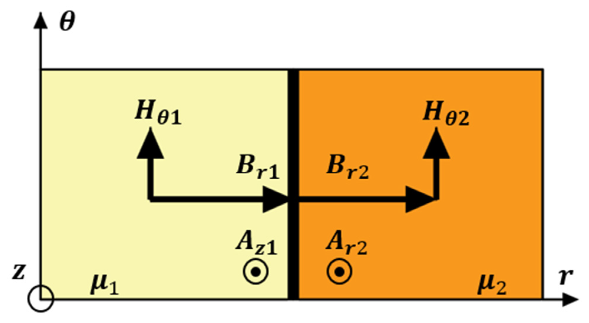
2.2. Boundary Conditions Principle

In Figure 4 without magnet excitation, the boundary condition between two adjacent materials is applied based on three principles: H_θ1 = H_θ2, B_r1 = B_r2, and A_z1 = A_z2. For mathematical convenience, it is preferable to choose the first and third principles, and rewrite them in terms of vector potential as follows:

$$\frac{\partial A_{z1}}{{\mu }_1\partial r}=\frac{\partial A_{z2}}{{\mu }_2\partial r}$$

(9)

$$A_{z1}=A_{z2}$$

(10)

where µ₁ and µ₂ are the relative permeability of the first and second materials, respectively.

If the first material is the magnet, then (9) turns out as follows:

$$\frac{\partial A_{z1}}{{\mu }_1\partial r}+{\mu }_0{M}_{\theta }=\frac{\partial A_{z2}}{{\mu }_2\partial r}$$

(11)

In Figure 1b, the continuity of the radial components of the vector potential leads to twelve following boundary conditions.

$$r=R_7\to \frac{\partial A_z^I}{{\mu }_r\partial r}+{\mu }_0{M}_{\theta }=0$$

(12)

$$r=R_6\to \left\{\begin{array}{c}\frac{\partial A_z^I}{{\mu }_r\partial r}+{\mu }_0{M}_{\theta }=\frac{\partial A_z^{II}}{\partial r}\\ A_z^{II}=A_z^I\end{array}\right.$$

(13)

$$r=R_5\to \left\{\begin{array}{c}\frac{\partial A_z^{II}}{\partial r}={\displaystyle \sum _{p=\mathrm{1,2}}^{P_m}}\frac{\partial A_z^p}{\partial r}\\ A_z^p=A_z^{II}\end{array}\right.$$

(14)

$$r=R_4\to \left\{\begin{array}{c}{A}_z^p=A_z^{III}\\ \frac{\partial A_z^{III}}{\partial r}={\displaystyle \sum _{p=\mathrm{1,2}}^{P_m}}\frac{\partial A_z^p}{\partial r}\end{array}\right.$$

(15)

$$r=R_3\to \left\{\begin{array}{c}\frac{\partial A_z^{III}}{\partial r}={\displaystyle \sum _{i=\mathrm{1,2}}^Q}\frac{\partial A_z^i}{\partial r}\\ A_z^i=A_z^{III}\end{array}\right.$$

(16)

$$r=R_2\to \left\{\begin{array}{c}{A}_z^i=A_z^j\\ \frac{\partial A_z^j}{\partial r}=\frac{\partial A_z^i}{\partial r}\end{array}\right.$$

(17)

$$r=R_1\to \frac{\partial A_z^j}{\partial r}=0$$

(18)

The coefficients were determined using a Fourier series expansion shown in Appendix A and Appendix B. The flux density at the air gap, then, is deduced from:

$$B_r=\frac{\partial A_z}{r\partial \theta };B_{\theta }=-\frac{\partial A_z}{\partial r}$$

(19)

2.3. The Maxwell Stress Tensor

The Maxwell stress tensor is given by the following equation:

$$\begin{array}{c}\hfill {\mathit{\sigma }}_{\mathit{i}\mathit{j}}=\frac{1}{{\mu }_0}(B_i{B}_j-\frac{1}{2}{\delta }_{ij}{\left|\overrightarrow{B}\right|}^2)\hfill \\ \mathrm{where}\hfill \\ \hfill {\delta }_{ij}=\left[\begin{array}{c}0\leftrightarrow i\ne j\\ 1\leftrightarrow i=j\end{array}\right.\hfill \end{array}$$

(20)

Applying 3D cylinder coordinates, Equation (20) turns out as such:

$${\mathit{\sigma }}_{\mathit{i}\mathit{j}}=\left[\begin{array}{ccc}{\sigma }_{rr}& {\sigma }_{\theta r}& {\sigma }_{zr}\\ {\sigma }_{r\theta }& {\sigma }_{\theta \theta }& {\sigma }_{z\theta }\\ {\sigma }_{rz}& {\sigma }_{\theta z}& {\sigma }_{zz}\end{array}\right]=\left[\begin{array}{ccc}\frac{B_r^2-B_{\theta }^2}{2{\mu }_0}& \frac{B_{\theta }{B}_r}{{\mu }_0}& 0\\ \frac{B_r{B}_{\theta }}{{\mu }_0}& \frac{-B_r^2+B_{\theta }^2}{2{\mu }_0}& 0\\ 0& 0& -\frac{B_r^2+B_{\theta }^2}{2{\mu }_0}\end{array}\right]$$

(21)

The force exerted over a surface S can be expressed as follows:

$$\mathit{F}=\int {\mathit{\sigma }}_{\mathit{i}\mathit{j}}d{S}_n=\int \left[\begin{array}{ccc}\frac{B_r^2-B_{\theta }^2}{2{\mu }_0}& \frac{B_{\theta }{B}_r}{{\mu }_0}& 0\\ \frac{B_r{B}_{\theta }}{{\mu }_0}& \frac{-B_r^2+B_{\theta }^2}{2{\mu }_0}& 0\\ 0& 0& -\frac{B_r^2+B_{\theta }^2}{2{\mu }_0}\end{array}\right]\left[\begin{array}{c}{dS}_r\\ {dS}_{\theta }\\ d{S}_z\end{array}\right]=\left[\begin{array}{c}\int \frac{B_r^2-B_{\theta }^2}{2{\mu }_0}d{S}_r+\int \frac{B_{\theta }{B}_r}{{\mu }_0}d{S}_{\theta }\\ \int \frac{B_r{B}_{\theta }}{{\mu }_0}d{S}_r+\int \frac{-B_r^2+B_{\theta }^2}{2{\mu }_0}d{S}_{\theta }\\ \int -\frac{B_r^2+B_{\theta }^2}{2{\mu }_0}d{S}_z\end{array}\right]$$

(22)

Generally, the attraction force consists of three surface directions in the integral. However, along the z-axis, the force density is constant, resulting in a zero integral for the z-directional force. Additionally, when compared to the radial force density, the force density in the $\theta$-direction is relatively small and can be neglected. As a result, the average force density acting on the modulation can be simplified as follows:

$$\mathit{\sigma }=\left[\begin{array}{c}{\sigma }_r\\ {\sigma }_{\theta }\\ {\sigma }_z\end{array}\right]=\left[\begin{array}{c}{\left.{\left.\frac{B_r^2-B_{\theta }^2}{2{\mu }_0}\right|}_{R_5}-\frac{R_4}{R_5}\frac{B_r^2-B_{\theta }^2}{2{\mu }_0}\right|}_{R_4}\\ {\left.{\left.\frac{B_r{B}_{\theta }}{{\mu }_0}\right|}_{R_5}-\frac{R_4}{R_5}\frac{B_r{B}_{\theta }}{{\mu }_0}\right|}_{R_4}\\ 0\end{array}\right]$$

(23)

As shown in Figure 8b, during the mechanical modulation analysis, the tangential component of the average magnetic force density appears notably smaller compared to the radial counterpart, often rendering it negligible in the analysis.

The electromagnetic torque is derived using the Maxwell stress tensor. An integration path along a circle with a radius within the air gap subdomain is employed, leading to the electromagnetic torque presentation as detailed in [35].

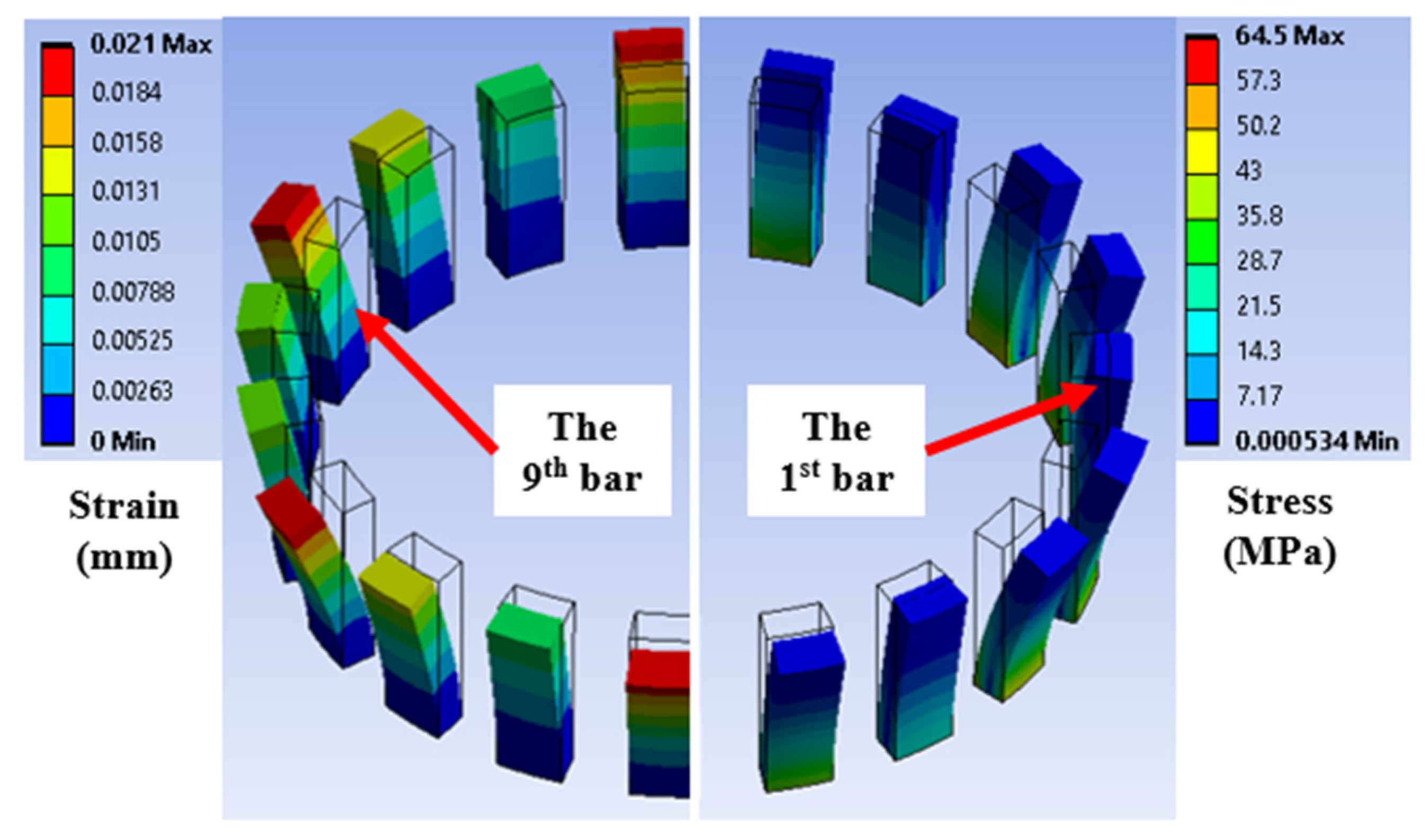
3. Stress and Deformation Analysis in Modulation

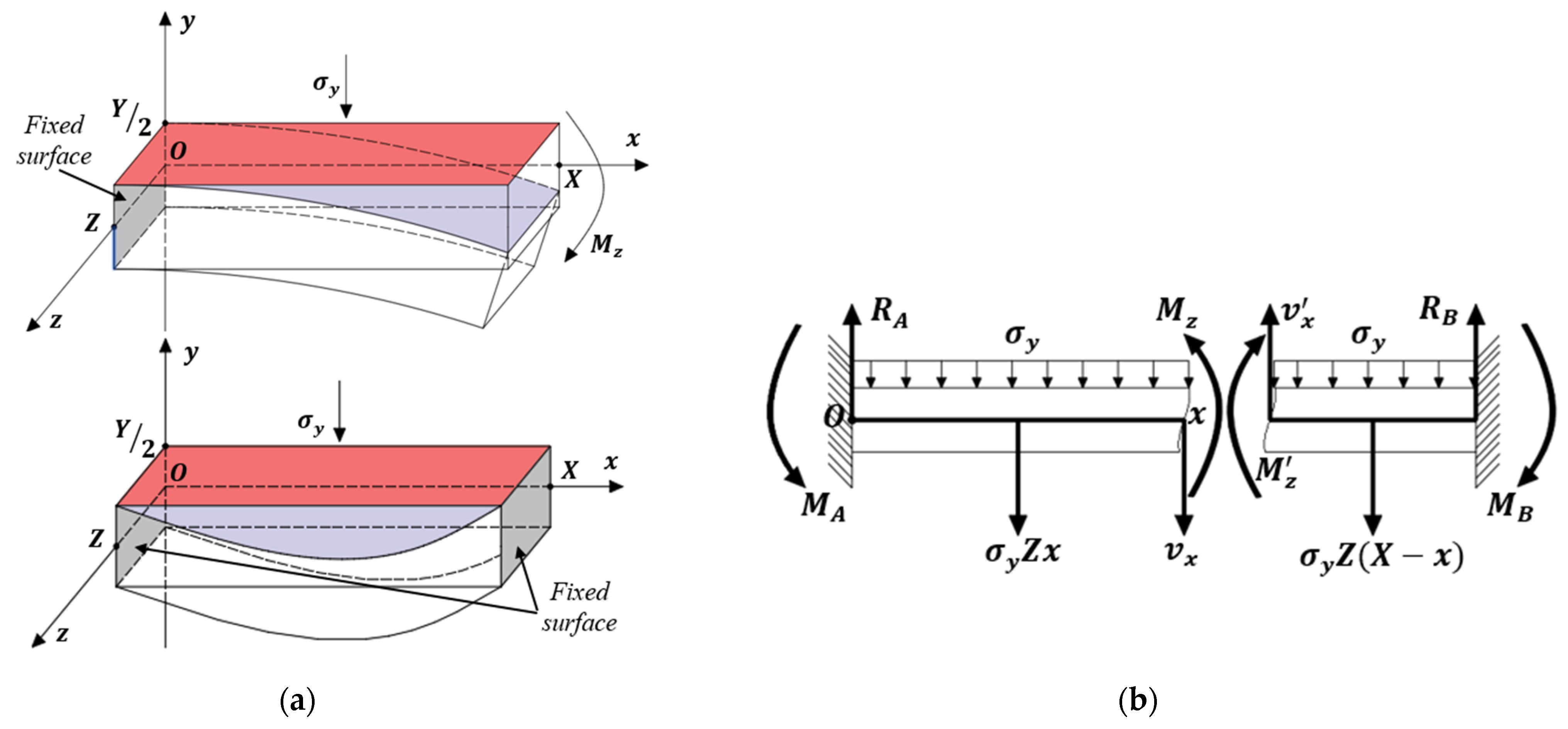
3.1. Timoshenko Beam Model

In the beginning, in order to simplify the model shown in Figure 5, the following assumptions are made:

• The coordinate $Or\theta z$ is converted into $Oxyz$;
• The cross section and material properties of the beam are constant along the length;
• There is a symmetrical cross-section about x-y plane;
• The height, width, and length of a converted bar are denoted as X, Y, and Z.

The model depicted in Figure 5b is commonly known as the Euler–Bernoulli beam, which assumes that both sides of the beam are free. However, in reality, in machines, one or both sides of the beam shown in Figure 6 may be fixed. This difference between mathematical computation and finite element method (FEM) simulation introduces a significant error, especially when the y-axis thickness (Y) is sufficiently large.

To address this problem, a Timoshenko beam model is introduced in [42]. The Timoshenko beam model takes into account the effect of shear deformation, providing a more accurate representation of the actual behavior of beams with fixed ends. Through incorporating the Timoshenko beam model, the error caused by the assumption of free ends in the Euler–Bernoulli beam model can be minimized. When applying a moment, M_z, on a surface area, A, and coefficients are given as in Table 1, the PDEs of the beam model are expressed as follows:

$$\left\{\begin{array}{c}\frac{dy}{dx}={\theta }_x+\frac{1}{\kappa AG}\frac{d{M}_z}{dx}\\ \frac{d{\theta }_x}{dx}=-\frac{M_z}{E{I}_z}\end{array}\right.$$

(24)

where ${\theta }_x$ is the angle of rotation of the normal to the mid-surface of the beam, and the second moment of area, $I_z$, is calculated similarly for both cases in Figure 6.

$$I_z=\frac{Y^{3}Z}{12}$$

(25)

3.2. Modulation Fixed at One End

Considering an arbitrary point along the beam that divides it into two sections, as shown in Figure 6b, our focus lies on the case where one side of the beam is fixed. In this scenario, we exclusively examine the left-side portion. The distribution of the moment acting along the modulation can be described using the following equation:

$$M_{zx}={\sigma }_{y}Z\frac{{-(X-x)}^2}{2}$$

(26)

Substituting (26) into (24), then combining the first boundary condition ${\theta }_{x=0}=0$, the angle, ${\theta }_x$, is derived as:

$${\theta }_x=-\frac{{\sigma }_{y}Z}{E{I}_z}\frac{{(X-x)}^3}{6}+\frac{{\sigma }_{y}Z}{E{I}_z}\frac{X^3}{6}$$

(27)

Through applying the second boundary condition $y_{x=0}=0$ for Equation (24), the deformation along the length of the modulation can be defined as follows:

$$y=\frac{{\sigma }_{y}Z}{E{I}_z}\frac{{\left(X-x\right)}^4}{24}+\frac{{\sigma }_{y}Z}{E{I}_z}\frac{X^{3}x}{6}+\frac{{\sigma }_{y}Z}{\kappa AG}\frac{{-\left(X-x\right)}^2}{2}-\frac{{\sigma }_{y}Z}{E{I}_z}\frac{X^4}{24}+\frac{{\sigma }_{y}Z}{\kappa AG}\frac{X^2}{2}$$

(28)

Under uniform stress acting in the y-direction, the stress distribution in the Oxy plane is calculated as:

$${\sigma }_y=\frac{y{M}_{zx}}{I_z}=-y{\sigma }_{y}Z\frac{{(X-x)}^2}{2}$$

(29)

3.3. Modulation Fixed at Both Ends

In the scenario of modulation fixed at both ends, both sections are required. Similar to Section 3.2, the following expressions apply:

$$M_{zx}={\sigma }_{y}Z\left(\frac{Xx}{2}-\frac{x^2}{2}-\frac{X^2}{12}\right)$$

(30)

$${\theta }_x=\frac{{\sigma }_{y}Z}{E{I}_z}\left(\frac{x^3}{6}-\frac{X{x}^2}{4}+\frac{X^{2}x}{12}\right)$$

(31)

Notably, because of symmetry along the center of the beam, the conditions, therefore, become ${\theta }_{x=\{0;X\}}=0$ and $y_{x=\{0;X\}}=0$. The deformation and stress of modulation are given as follows:

$$y=\frac{{\sigma }_{y}Z}{E{I}_z}\frac{{\left(X-x\right)}^2{x}^2}{24}+\frac{{\sigma }_{y}Z}{\kappa AG}\frac{x(X-x)}{2}$$

(32)

$${\sigma }_y=\frac{y{M}_{zx}}{I_z}=\frac{y{\sigma }_{y}Z}{I_z}\left(\frac{Xx}{2}-\frac{x^2}{2}-\frac{X^2}{12}\right)$$

(33)

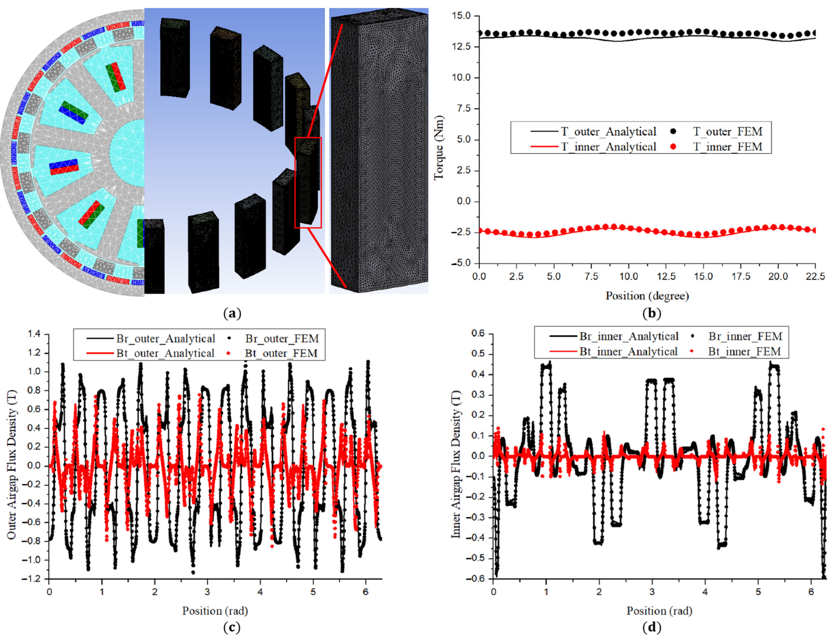
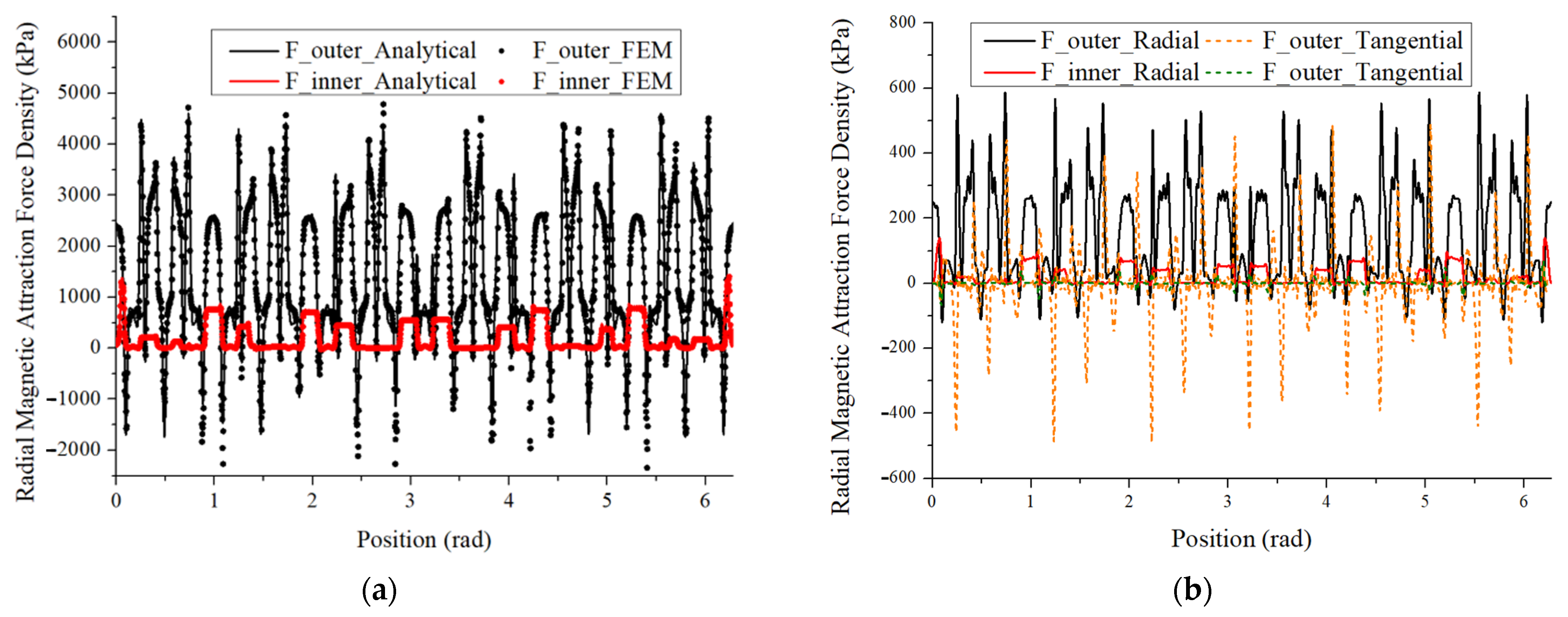
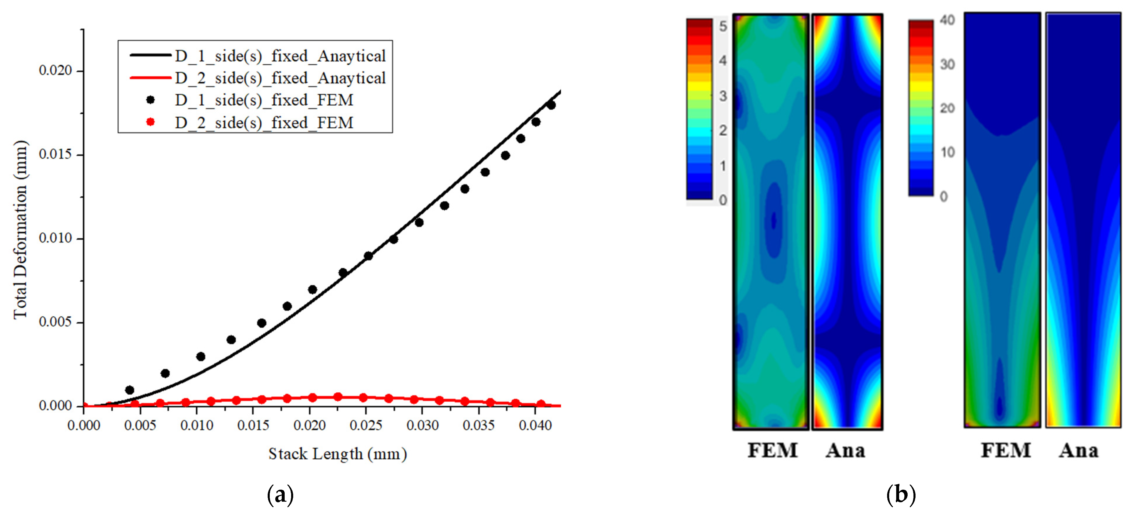
4. Results and Discussion

An example, with parameters detailed in Table 2 and material characteristics presented in Table 1, was subjected to FEM simulation and analytical analysis. Notably, the FEM mesh for both electromagnetic and mechanical analyses is illustrated in Figure 7a.

The electromagnetic torque, air gap flux densities, and magnetic force density obtained through the analytical method aligned closely with FEM simulation results, as depicted in Figure 7b–d and Figure 8a. The tangential component of the average magnetic force density is approximately zero in Figure 8b. This leads to the neglect of tangential components in stress analysis in this study. The non-uniform force distribution is apparent in these figures, contributing to uneven deformation in the modulations.

Figure 9 shows non-uniform deformation as well as stress in bars. The first bar has almost no significant influence from the magnetic force, whereas an extreme bend is occupied in the ninth bar.

Generally, there is a strong agreement between the mathematical method and FEM results, as depicted in Figure 10, which presents deformation and stress profiles. In the case of two fixed ends (depicted in Figure 10b), although the stress distribution along the bar is not entirely consistent, the maximum stress at the four corners is accurately predicted. Notably, the scenario with two fixed ends exhibits greater stability in comparison to the case with only one fixed end. In the latter, the maximum deformation and stress are approximately 1/20 and 1/8 times larger, respectively.

5. Conclusions

The proposed mathematical method was an efficient approach for obtaining mechanical characteristics in the modulation. Moreover, compared with 2D magnetic attraction force and 3D stress/deformation FEM simulations, the computational time of the mathematical method was reduced from 30 s and 5 min to 2 s and 1.5 s, respectively. This allows designers to apply optimization techniques that save time exponentially.

Continuing research based on this paper can be outlined as follows:

• Consider the non-linear characteristic of magnetic material;
• Consider the skin effect for the solid modulation;
• The influence of the on-load or unbalanced load should be ideal;
• Verify the subdomain method with the test bench’s results;
• Develop a mathematical method for a lamination-structured modulation.

References

1. Wang, Q.; Zhao, X.; Niu, S. Flux-Modulated Permanent Magnet Machines: Challenges and Opportunities. World Electr. Veh. J. 2021, 12, 13. [Google Scholar] [CrossRef]
2. Padinharu, D.K.K. Permanent Magnet Vernier Machines for Direct-Drive Offshore Wind Power: Benefits and Challenges. IEEE Access 2022, 10, 20652–20668. [Google Scholar] [CrossRef]
3. Zhu, Z.Q. Overview of novel magnetically geared machines with partitioned stators. IET Electr. Power Appl. 2018, 12, 595–604. [Google Scholar] [CrossRef]
4. Wang, L.L.; Shen, J.X.; Luk, P.C.K.; Fei, W.Z.; Wang, C.F.; Hao, H. Development of a Magnetic-Geared Permanent-Magnet Brushless Motor. IEEE Trans. Magn. 2009, 45, 4578–4581. [Google Scholar] [CrossRef]
5. Niu, S.; Ho, S.L.; Fu, W.N. A Novel Direct-Drive Dual-Structure Permanent Magnet Machine. IEEE Trans. Magn. 2010, 46, 2036–2039. [Google Scholar] [CrossRef]
6. Jian, L.; Xu, G.; Mi, C.C.; Chau, K.T.; Chan, C.C. Analytical Method for Magnetic Field Calculation in a Low-Speed Permanent-Magnet Harmonic Machine. IEEE Trans. Energy Convers 2011, 26, 862–870. [Google Scholar] [CrossRef]
7. Gerber, S.; Wang, R.J. Design and Evaluation of a Magnetically Geared PM Machine. IEEE Trans. Magn. 2015, 51, 8107010. [Google Scholar] [CrossRef]
8. Fu, W.N.; Ho, S.L. A Quantitative Comparative Analysis of a Novel Flux-Modulated Permanent-Magnet Motor for Low-Speed Drive. IEEE Trans. Magn. 2010, 46, 127–134. [Google Scholar] [CrossRef]
9. Jing, L.; Tang, W.; Wang, T.; Ben, T.; Qu, R. Performance Analysis of Magnetically Geared Permanent Magnet Brushless Motor for Hybrid Electric Vehicles. IEEE Trans. Transp. 2022, 8, 2874–2883. [Google Scholar] [CrossRef]
10. Jing, L.; Pan, Y.; Wang, T.; Qu, R.; Cheng, P.T. Transient Analysis and Verification of a Magnetic Gear Integrated Permanent Magnet Brushless Machine With Halbach Arrays. IEEE Trans. Emerg. Sel. Topics Power Electron. 2022, 10, 1881–1890. [Google Scholar] [CrossRef]
11. Jing, L.; Tang, W.; Liu, W.; Rao, Y.; Tan, C.; Qu, R. A Double-Stator Single-Rotor Magnetic Field Modulated Motor with HTS Bulks. IEEE Trans. Appl. Supercond. 2022, 32, 5201105. [Google Scholar] [CrossRef]
12. Atallah, K.; Rens, J.; Mezani, S.; Howe, D. A Novel “Pseudo” Direct-Drive Brushless Permanent Magnet Machine. IEEE Trans. Magn. 2008, 44, 4349–4352. [Google Scholar] [CrossRef]
13. Okada, K.; Niguchi, N.; Hirata, K. Analysis of a Vernier Motor with Concentrated Windings. IEEE Trans. Magn. 2013, 49, 2241–2244. [Google Scholar] [CrossRef]
14. Liu, W.; Thomas, A.L. Analysis of Consequent Pole Spoke Type Vernier Permanent Magnet Machine with Alternating Flux Barrier Design. IEEE Trans. Ind. Appl. 2018, 54, 5918–5929. [Google Scholar] [CrossRef]
15. Li, D.; Ronghai, Q.; Thomas, A.L. High-Power-Factor Vernier Permanent-Magnet Machines. IEEE Trans. Ind. Appl. 2014, 50, 3664–3674. [Google Scholar] [CrossRef]
16. Li, D.; Qu, R.; Li, J.; Xiao, L.; Wu, L.; Xu, W. Analysis of Torque Capability and Quality in Vernier Permanent-Magnet Machines. IEEE Trans. Ind. Appl. 2016, 52, 125–135. [Google Scholar] [CrossRef]
17. Jing, L.; Gong, J.; Huang, Z.; Ben, T.; Huang, Y. A New Structure for the Magnetic Gear. IEEE Access 2019, 7, 75550–75555. [Google Scholar] [CrossRef]
18. Jing, L.; Huang, Z.; Chen, J.; Qu, R. Design, Analysis, and Realization of a Hybrid-Excited Magnetic Gear During Overload. IEEE Trans. Ind. Appl. 2020, 56, 4812–4819. [Google Scholar] [CrossRef]
19. Ling, Z.; Zhao, W.; Ji, J.; Xu, M. Design and Analysis of a Magnetic Field Screw Based on 3-D Magnetic Field Modulation Theory. IEEE Trans. Energy Convers. 2022, 37, 2620–2628. [Google Scholar] [CrossRef]
20. Jing, L.; Liu, W.; Tang, W.; Qu, R. Design and Optimization of Coaxial Magnetic Gear With Double-Layer PMs and Spoke Structure for Tidal Power Generation. IEEE ASME Trans. Mechatron. 2023. [Google Scholar] [CrossRef]
21. Jing, L.; Wang, T.; Tang, W.; Liu, W.; Qu, R. Characteristic Analysis of the Magnetic Variable Speed Diesel–Electric Hybrid Motor with Auxiliary Teeth for Ship Propulsion. IEEE ASME Trans Mechatron 2023. [Google Scholar] [CrossRef]
22. Liu, Y.; Fu, W.N.; Ho, S.L.; Niu, S.; Ching, T.W. Electromagnetic Performance Analysis of Novel HTS Doubly Fed Flux-Modulated Machines. IEEE Trans. Appl. Supercond. 2015, 25, 5203204. [Google Scholar] [CrossRef]
23. Wang, Q.; Niu, S.; Yang, S. Design Optimization and Comparative Study of Novel Magnetic-Geared Permanent Magnet Machines. IEEE Trans. Magn. 2017, 53, 8104204. [Google Scholar] [CrossRef]
24. Wang, Y.; Niu, S.; Fu, W. Sensitivity Analysis and Optimal Design of a Dual Mechanical Port Bidirectional Flux-Modulated Machine. IEEE Ind. Electron. 2018, 65, 211–220. [Google Scholar] [CrossRef]
25. Yousefnejad, S.; Heydari, H.; Akatsu, K.; Ro, J.S. Analysis and Design of Novel Structured High Torque Density Magnetic-Geared Permanent Magnet Machine. IEEE Access 2021, 9, 64574–64586. [Google Scholar] [CrossRef]
26. Niu, S.; Sheng, T.; Zhao, X.; Zhang, X.D. Operation Principle and Torque Component Quantification of Short-Pitched Flux-Bidirectional-Modulation Machine. IEEE Access 2019, 7, 136676–136685. [Google Scholar] [CrossRef]
27. Liu, Y.; Zhu, Z.Q. Influence of Gear Ratio on the Performance of Fractional Slot Concentrated Winding Permanent Magnet Machines. IEEE Ind. Electron. 2019, 66, 7593–7602. [Google Scholar] [CrossRef]
28. Jing, L.; Liu, L.; Xiong, M.; Feng, D. Parameters Analysis and Optimization Design for a Concentric Magnetic Gear Based on Sinusoidal Magnetizations. IEEE Trans. Appl. Supercond. 2014, 24, 0600905. [Google Scholar]
29. Jing, L.; Su, Z.; Wang, T.; Wang, Y.; Qu, R. Multi-Objective Optimization Analysis of Magnetic Gear with HTS Bulks and Uneven Halbach Arrays. IEEE Trans. Appl. Supercond. 2023, 33, 5202705. [Google Scholar] [CrossRef]
30. Wang, Y.; Jing, L. A Novel Eccentric Harmonic Magnetic Gear with Inhomogeneous Structure and Halbach Array. In Proceedings of the 2022 IEEE 3rd China International Youth Conference on Electrical Engineering (CIYCEE), Wuhan, China, 3–5 November 2022; pp. 1–6. [Google Scholar]
31. Lee, J.I.; Shin, K.H.; Bang, T.K.; Ryu, D.W.; Kim, K.H.; Hong, K.; Choi, J.Y. Design and Analysis of the Coaxial Magnetic Gear Considering the Electromagnetic Performance and Mechanical Stress. IEEE Trans. Appl. Supercond. 2020, 30, 3700105. [Google Scholar] [CrossRef]
32. Modaresahmadi, S.; Barnett, D.; Baninajar, H.; Bird, J.Z.; Williams, W.B. Structural modeling and validation of laminated stacks in magnetic gearing applications. Int. J. Mech. Sci. 2021, 192, 106133. [Google Scholar] [CrossRef]
33. Devillers, E.; Besnerais, J.L.; Lubin, T.; Hecquet, M.; Lecointe, J.P. A review of subdomain modeling techniques in electrical machines: Performances and applications. In Proceedings of the 2016 XXII International Conference on Electrical Machines (ICEM), Lausanne, Switzerland, 4–7 September 2016. [Google Scholar]
34. Zhu, Z.Q.; Howe, D. Instantaneous magnetic field distribution in brushless permanent magnet DC motors. III. Effect of stator slotting. IEEE Trans. Magn. 1993, 29, 143–151. [Google Scholar] [CrossRef]
35. Lubin, T.; Mezani, S.; Rezzoug, A. 2-D Exact Analytical Model for Surface-Mounted Permanent-Magnet Motors with Semi-Closed Slots. IEEE Trans. Magn. 2011, 47, 479–492. [Google Scholar] [CrossRef]
36. Shen, Y.; Zhu, Z.Q. General analytical model for calculating electromagnetic performance of permanent magnet brushless machines having segmented Halbach array. IET Electr. Syst. Transp. 2013, 3, 57–66. [Google Scholar] [CrossRef]
37. Lubin, T.; Mezani, S.; Rezzoug, A. Analytical Computation of the Magnetic Field Distribution in a Magnetic Gear. IEEE Trans. Magn. 2010, 46, 2611–2621. [Google Scholar] [CrossRef]
38. Lubin, T.; Mezani, S.; Rezzoug, A. Development of a 2-D Analytical Model for the Electromagnetic Computation of Axial-Field Magnetic Gears. IEEE Trans. Magn. 2013, 49, 5507–5521. [Google Scholar] [CrossRef]
39. Jing, L.; Gong, J.; Ben, T. Analytical Method for Magnetic Field of Eccentric Magnetic Harmonic Gear. IEEE Access 2020, 8, 34236–34245. [Google Scholar] [CrossRef]
40. Dubas, F.; Boughrara, K. New Scientific Contribution on the 2-D Subdomain Technique in Polar Coordinates: Taking into Account of Iron Parts. Math. Comput. Appl. 2017, 22, 42. [Google Scholar] [CrossRef]
41. Guo, B.; Djelloul-Khedda, Z.; Dubas, F. Nonlinear Analytical Solution in Axial Flux Permanent Magnet Machines using Scalar Potential. IEEE Ind. Electron. 2023. [Google Scholar] [CrossRef]
42. Öchsner, A. Timoshenko Beam Theory. In Classical Beam Theories of Structural Mechanics; Springer: Cham, Switzerland, 2021; pp. 67–104. [Google Scholar]
Figure 1. (a) Configuration and (b) simplified model of the MGGs.
Machines 11 00887 g001
Figure 2. The parallel magnetic magnetization illustration.
Machines 11 00887 g002
Figure 3. Winding layouts: non-overlapping (top) and overlapping (bottom) windings.
Machines 11 00887 g003
Figure 4. Boundary condition principle.
Machines 11 00887 g004
Figure 5. (a) The stress tensor in a 3D space O x y z and O r θ z . (b) The general beam.
Machines 11 00887 g005
Figure 6. (a) An illustration of the modulation being deformed one side and two sides and (b) their simplified model for the mathematical solution.
Machines 11 00887 g006
Figure 7. (a) A 2D model for magnetic attraction force analysis (33,450 mesh elements) and a 3D model for stress/deformation analysis (632,268 mesh elements); (b) the electromagnetic torque in the outer air gap and inner air gap; the air gap flux density in the (c) outer air gap and (d) inner air gap.
Machines 11 00887 g007
Figure 8. (a) The radial magnetic attraction force density; (b) the radial and tangential magnetic force density in the outer and inner air gap.
Machines 11 00887 g008
Figure 9. Mechanical analysis using the FEM of the model with one end fixed.
Machines 11 00887 g009
Figure 10. The ninth modulation bar comparison between analytical method and FEM simulation of (a) deformation, stress of model with (b) one end fixed (right), and both ends fixed (left).
Machines 11 00887 g010