Simultaneous Fault Diagnostics for Three-Shaft Industrial Gas Turbine

Abstract

The study focused on the development of -gas turbine full- and part-load operation diagnostics. The gas turbine performance model was developed using commercial software and validated using the engine manufacturer data. Upon the validation, fouling, erosion, and variable inlet guide vane drift were simulated to generate faulty data for the diagnostics development. Because the data from the model was noise-free, sensor noise was added to each of the diagnostic set parameters to reflect the actual scenario of the field operation. The data was normalized. In total, 13 single, and 61 double, classes, including 1 clean class, were prepared and used as input. The number of observations for single faults diagnostics were 1092, which was 84 for each class, and 20,496 for double faults diagnostics, which was 336 for each class. Twenty-eight machine learning techniques were investigated to select the one which outperformed the others, and further investigations were conducted with it. The diagnostics results show that the neural network group exhibited better diagnostic accuracy at both full- and part-load operations. The test results and its comparison with literature results demonstrated that the proposed method has a satisfactory and reliable accuracy in diagnosing the considered fault scenarios. The results are discussed, following the plots.

1. Introduction

The performance of the gas-path components, particularly the compressor and turbine, is critical to the overall performance of the engine, and the health status of these components needs high attention, due to their vulnerability to various internal and external degradation factors [1]. Performance degradation of the GT can be either temporary or permanent. Temporary degradation can be partly recovered during operation and/or engine overhaul, but permanent degradation means that the component needs to be replaced [2]. Fouling, erosion, corrosion, and blade tip clearance are among the temporary degradation causes, whereas mechanical misalignment, lack of oil for lubrication, airfoil distortion, lead to permanent deterioration. Deterioration can be categorized as recoverable (with washing), non-recoverable (cannot be recovered by washing during operation, but recoverable during overhaul), and permanent (not recoverable by either washing or overhaul) [3]. Related to the service period of the engine or the evolution time frame of the deterioration, performance deterioration can also be classified into short-term/rapid and long-term/gradual deterioration [4]. Short-term/rapid deterioration often happens at the early age of the gas turbine engine as it starts its operation, or it may be the result of a single event, such as object damage at any time during the engine’s operation. On the other hand, long-term deterioration is formed more gradually, and is often due to the ingestion and accumulation of different contaminants and/or high operating temperature.

Researchers have conclusively demonstrated that fouling and erosion are the predominant issues frequently encountered in gas turbines [5]. These two faults, fouling and erosion, have been identified as the primary causes of performance degradation and operational inefficiencies in gas turbine systems. Even though fouling and erosion are the primary faults found in gas turbines, some other faults have also been found to occur, including corrosion, blade tip clearance, and foreign and domestic object damage. As shown in

Table 1. Summary of GT degradation component performance change indicators.

GT Physical Fault	Compressor and Turbine Performance Change Indication	Reference
Fouling	↓ Compressor and turbine Γ ↓ Pressure ratio (PR) ↓ Compressor and turbine η	[6,7,8,9,10,11,12,13,14]
Erosion	↓ Compressor Γ ↑ Turbine Γ ↓ Compressor pressure ratio ↓ Compressor and turbine η	[8,15,16,17,18]
Corrosion	↓ Compressor Γ and η ↑ Turbine Γ ↓ Turbine η	[5,16,19,20,21]
Blade tip clearance	↓ Compressor and turbine η ↓ Compressor and turbine Γ	[5,22,23]
Foreign and domestic object damage	↓ Compressor and turbine η ↑/↓ Compressor and turbine Γ ↓ Compressor pressure ratio	[9,16,24]

, these physical faults cause changes in one or more of the performance parameters which describe an individual gas-path component’s performance. The performance parameters generally include compressor flow capacity, compressor isentropic efficiency, turbine flow capacity, and turbine isentropic efficiency. Changes in the performance parameters cause consequent changes in the measurement parameters (temperature, pressure, shaft speed, and fuel flow), which are the fault indicators or symptoms in engine health monitoring.

Case Engine

The Rolls-Royce RB211-24G three-shaft gas turbine which is manufactured by Rolls Rolls-Royce, Goodwood, England, is used as a case engine in this study. This gas turbine engine was developed by Rolls-Royce, a British engineering company known for its high-quality engines used in aerospace and other applications. The gas turbine engine is also called a high-pressure ratio engine. The gas generator has two spools (meaning two rotors), and its exhaust gases drive the power turbine. The secondary air taken from the gas generator compressors serve as cooling and sealing air. The gas turbine has six main gas-path components, including an intermediate-pressure compressor (IPC), a high-pressure compressor (HPC), a combustion chamber, a high-pressure turbine (HPT), an intermediate-pressure turbine (IPT), and a power turbine (PT) [25]. Three-shaft industrial gas turbine configurations are shown in Figure 1.

The three-shaft gas turbine consists of a gas generator, with two shafts, and a power turbine, with a single shaft. The gas generator consists of a seven-stage intermediate-pressure compressor, a six-stage high-pressure compressor, a single-stage high-pressure turbine, and a single-stage intermediate-pressure turbine. The intermediate-pressure and high-pressure shafts are separated and operate at their respective optimal speeds. The intermediate-pressure compressor is driven by the intermediate-pressure turbine, whereas the high-pressure compressor is driven by the high-pressure turbine. That means the intermediate-pressure compressor and intermediate-pressure turbine share the intermediate-speed shaft, whereas the high-pressure compressor and the high-pressure turbine share the high-speed shaft. As for the power turbine, it is a double-stage free axial turbine.

The laws of thermodynamics are always used to investigate gas turbine performance. An industrial gas turbine has a compressor, combustor, and turbine [26]. Furthermore, every open and closed-cycle power generation gas turbine works in four processes, which are: compression, combustion, expansion, and heat rejection [27]. Air is used as a medium of fluid for the gas turbine, and is compressed at the compressor, while combustion takes place at the combustor. The result of combustion gases will be then entered into the expander or turbines for production of power. Gas turbine systems work by the Brayton cycle principle [28]. The ideal Brayton cycle is defined as a thermodynamic cycle that consists of an isentropic and adiabatic compression of a gas, followed by an addition of heat at constant pressure and an energy extraction that results in gaseous expansion [26], as shown in Figure 2 below.

2. Fault Diagnostics

Fault diagnosis is the process of identifying and determining the root cause of problems or faults that occur in a machine or system [29]. This process involves analyzing data and signals from various sensors, such as temperature sensors, vibration sensors, pressure sensors, and others, to detect anomalies or deviations from no-fault operating conditions. The goal of fault diagnosis is to quickly and accurately diagnose the problem in order to minimize downtime and reduce repair costs [30,31]. This can be accomplished by using various techniques, such as statistical analysis, machine learning, and artificial intelligence, to detect patterns and anomalies in the data. Fault diagnosis is, in general, the procedure of detecting, isolating, and identifying an impending or incipient failure condition, during which the affected component is still operational, though in a degraded mode [32]. Fault diagnosis is used in a variety of industries, including manufacturing, transportation, energy, and healthcare, where it plays a critical role in ensuring the safe and efficient operation of machines and systems [33]. The general engine diagnosis approach is shown in Figure 1.

Fault Detection: The process of detecting or identifying the occurrence of a fault or anomaly in a system. This involves monitoring that system to detect deviations from normal behavior, which may indicate the presence of a fault.

Fault Isolation: The process of identifying which component or subsystem in a system is responsible for a fault. This involves using various diagnostic techniques, such as testing, modeling, and analysis, to isolate the root cause of the problem.

Fault Identification: The process of analyzing data collected during fault detection and isolation phases to quantify the deterioration magnitude.

Gas Turbine Diagnostics Approaches

Over the years, extensive progress has been made by engine manufacturers and the research community in the field of gas turbine gas-path diagnostics [34,35]. Gas turbine diagnostic methods can be categorized into two groups: mechanical-based and performance-based approaches. Mechanical-based condition monitoring techniques, known as non-performance-based condition monitoring, involve various methods, including analysis of oil and wear debris, vibration analysis, acoustics, evaluation of lubrication flow parameters, thermography, load, and metal temperature analysis [36]. Non-performance-based condition monitoring for gas turbine diagnosis has been an area of continuous evolution for researchers [36,37]. However, the more advanced and cost-efficient method for assessing engine health conditions lies in performance-based monitoring, which investigates the degradation of engine performance using data-driven techniques. A study by Barad et al. confirms the crucial need to develop performance-based diagnoses in gas turbine diagnostics, highlighting the high significance of performance-based condition monitoring [38,39,40]. The most important components are the compressors and turbines, which are highly critical components in gas turbines. Consequently, researchers emphasize the degradation analyses of these components. Engine performance relies on the variation of gas-path measurements and component performance parameters [5]. To perform a thorough health assessment using a condition-based method, it is imperative to have access to detailed information about engine performance, as well as a comprehensive set of operating parameters. Additionally, careful estimation of the number of measurements is crucial, as improper estimation can lead to wrong solutions [41]. Identifying the sources of data and collecting the necessary data and information is the primary groundwork for developing a performance-based diagnostic model [42].

Performance-based health monitoring can be classified into two categories: model-based (MB) and data-driven/artificial intelligence-based approaches. The model-based technique is a highly adaptable model, capable of detecting unforeseen faults. Initially introduced by Urban and Escher [43,44], the linear and nonlinear GPA method served as the foundation for this technique. The diagnostic approach, based on the model-based technique, is thermodynamic computation. Through the utilization of thermodynamic equations, a range of parameters that rely on measurements, including pressure, temperature, output power, and fuel mass flow rate, along with performance indicators, such as component efficiency, air flow rate, and pressure ratio, can be mathematically calculated [45,46,47]. To implement the model-based engine health monitoring technique, a performance simulation algorithm or program is required, and the component characteristics of each engine must comply with the performance simulation. The component map, which simulates the engine’s performance, is the same as that of a real engine. However, the engine’s component maps are typically not accessible to users, due to manufacturer proprietary rights. Consequently, researchers in this field rely on scaled maps, which are available online and which closely resemble the characteristics of the actual engine. Failure to do so may lead to discrepancies between the off-design performance model and the real engine [48,49,50].

Model-based methods do not maintain perfectly on the sensor noise and bias problem. Due to this problem, a data-driven (artificial intelligence) method has emerged [51,52], which is also called a performance-based health monitoring approach, which successfully detects anticipated faults. Data-driven methods include Artificial Neural Network (ANN) [50,53,54,55,56], Fuzzy Logic (FL) [57,58,59,60], Bayesian Belief Network (BBN) [59,61,62,63], Deep Learning (DL) [64,65,66,67], Support Vector Machine (SVM) [39,68,69,70,71], K-Nearest Neighbor (KNN) [72,73,74] and Genetic Algorithm (GA) [75,76,77]. In the data-driven approaches, the data collected from the engine will be utilized to develop a diagnostic model. This model requires data from both healthy engine conditions and various faulty conditions to be effectively created [31]. There are three possible ways to gather the desired information: collecting data directly from the real engine throughout its lifespan, conducting tests, or using engine demonstration or modeling. Due to the high cost associated with collecting data directly from the engine and through tests, it is most recommended to consider gathering data from an engine model. Using the data generated from the performance model, a gas turbine diagnostic model can be developed and used to monitor the health status of the engine, as shown in Figure 3.

Some three-shaft data-driven diagnostics works have been found in the literature. Priya and Riti [78] have developed a three-shaft gas turbine diagnostics model using fuzzy logic. The benefits and challenges of using fuzzy logic to solve the gas turbine engine diagnostic problem was emphasized. The diagnostic model was used to detect engine sensor and component fault conditions. However, it was limited to fault detection and full-load operation. Joly et al. [79] proposed an artificial neural network-based diagnostics technique. Both single and double component faults were considered. The result proved that artificial neural networks are a promising tool for double component fault diagnosis. The study was limited to full-load operation and did not distinguish the types of physical faults, as they just considered a general fault. Ogaji et al. [80] have investigated fuzzy logic for three-shaft industrial gas turbine diagnostics. Measurements noises were considered and each of the single component faults were identified. However, this study was limited to single component faults diagnosis at full-load operation. Another study, conducted by Marinai et al. [81], investigated fuzzy logic for three-shaft aero gas turbine diagnostics. An application of the method to a three-shaft turbofan engine provided a promising result. The study focused exclusively on the engine’s performance during full-load operation. Sampath et al. [82] investigated a hybrid technique. This study’s aim was to accurately detect any deviations in the performance of components, as well as identify sensor faults. The proposed diagnostics technique combined two advanced techniques: the Genetic Algorithm and Artificial Neural Network. The nested neural network serves as a pre-processing mechanism or filter, effectively decreasing the number of fault classes that need to be examined by the genetic algorithm-based diagnostics model. By utilizing this hybrid model, the accuracy, reliability, and consistency of the obtained results were enhanced. However, the study was limited to full-load operation.

A three-shaft gas turbine diagnosis model was developed using artificial neural network by Loboda et al. [83]. The study conducted a comparison between two types of networks: a multilayer perceptron and a radial basis network. The multilayer perceptron is commonly used for gas turbine fault recognition, while some studies have highlighted the strong recognition capabilities of the radial basis network. Both networks were included in the study to assess their performance. The results indicate that the radial basis network is slightly more accurate than the perceptron. However, it requires significantly more computer memory and computation time compared to the perceptron. The study was on limited fault detection at full-load operation. Sina et al. [84] investigated a dynamic neural network based on the multilayer perceptron network for three-shaft gas turbine diagnostics. The detection and isolation process involved determining the difference between each network’s output and the measured engine output, which generated residuals. These residuals were then used to effectively diagnose faults. However, the study was still limited to single fault diagnostics at full-load operation. In another study, diagnostics development using artificial neural network for a three-shaft gas turbine was conducted by Mustagime and Kurt [85]. In this study, the authors developed a regression model to investigate the relationship between flight parameters and the Exhaust Gas Temperature (EGT) parameter. To accomplish this, they utilized multiple regression analysis, which allowed them to analyze how various flight parameters impact the EGT parameter. Finally, they proposed an advanced computational technique for accurate identification.

Mateus et al. [86] investigated fuzzy logic for three-shaft aircraft gas turbine diagnostics. The dataset used in this study was acquired by running simulations on the Propulsion Diagnostic Method Evaluation Strategy software developed by the National Aeronautics and Space Administration (NASA). To evaluate the performance of the proposed model, the results were compared to those obtained from a type-1 fuzzy classifier with rule extraction, using the Wang and Mendel method. The analysis of the results clearly demonstrated the effectiveness of the proposed model. The comparison to the Wang and Mendel fuzzy classifier proved that the proposed model achieved superior performance with fewer rules. However, the diagnosis model was limited to single component and sensor faults analysis. Amare et al. [87] developed a hybrid diagnostic method for a three-shaft gas turbine. In this study, an Adaptive Gas-Path Analysis (AGPA) was employed to correct measurement data for fluctuation due to ambient conditions. The corrected data was then utilized for the Bayesian network (BN)-based fault diagnostic development. The effectiveness of the proposed method was confirmed by the test results. However, in this study, only compressor fouling and turbine erosion were considered. In addition to this, the study was limited to single fault detection at full-load operation ( Zhouzheng et al. [88]).

After a comprehensive literature review, it is clearly seen that, in the previous three-shaft gas turbine diagnostics studies, variable inlet guide vane drift and part-load operations remain unconsidered. Variable inlet guide vanes are adjustable blades located at the compressor inlet, controlling the airflow entering the compressor. However, over time, these guide vanes can experience drift, meaning they may deviate from their intended position. This drift can result in altered aerodynamic conditions, affecting the efficiency and performance of the gas turbine. Therefore, this study’s aim is to develop a three-shaft gas turbine diagnostic model using data-driven techniques by considering both single and double component faults. Two physical faults, such as fouling and erosion at each of the gas-path components, and one malfunction, called variable inlet guide vane drift (both up- and down-drift), at both full- and part-load operation, have been considered in the diagnostics development.

3. Diagnostics Development

The diagnostics model consists of two main components: fault detection and isolation, and fault identification. Both are at full- and part-load operation. To develop these two models, the 10 best diagnostics set parameters were utilized. A total of 13 single and 61 double faults classes, including clean class, were considered. Detailed fault patterns for both single and double faults can be found in Chapter Three of this study. For the single faults, 1092 observations were taken, with each single fault having 84 observations. On the other hand, 20,496 observations for double faults were taken, with 336 observations for each double fault. It is worth noting that the data obtained from the model were initially noise-free. Hence, to simulate real-world field scenarios, sensor noise was introduced to each of the diagnostic set parameters. Following the addition of noise, the data were then normalized within the range of −1 to 1.

3.1. Procedure

The gas turbine design point output power is 26,025 kW. All the information about the gas turbine engine is presented in the published paper, [89]. In addition to this, the design point and off-design performance model were developed, validated, and presented in the same paper, which is our previous work. Once the gas turbine performance model was developed and validated as presented [89], the clean data was generated at both full- and part-load conditions (80% load and 90% load, respectively). Subsequently, physical faults were intentionally implanted and simulated to generate single and double faulty data, as well as both full- and part-load conditions. To simulate physical faults and generate faulty data, the relationship of physical faults and performance parameters presented in [18,90] was used. This approach allowed for a comprehensive study of the gas turbine’s performance under normal and faulty conditions, providing insights into its behavior and aiding in the development of an effective diagnostics model. The procedure of the diagnostics development is shown in Figure 4.

3.2. Selected Diagnostics Set Measurements

Measurement selection for diagnostic model development requires careful consideration. To effectively select the gas path measurements for diagnostic analysis, researchers have employed various selection criteria. For instance, Jasmani et al. [91] conducted a comprehensive analysis to identify the optimal gas path diagnostic set for the RB211-24G gas turbine. This analysis involved multiple steps, such as measurement classification analysis, measurement sensitivity analysis, measurement correlations analysis, and measurement subsets analysis. The researchers considered different types of faults, ranging from single faults to faults in all components of the gas turbine. Based on their analysis, they identified the top ten diagnostic sets for the RB211-24G gas turbine, which are listed in

Table 2. Selected diagnosis measurement parameters [91].

Parameters	Description
P24	LPC exit pressure
T24	LPC exit temperature
P3	HPC exit pressure
T3	HPC exit temperature
P43	HPT exit pressure
P47	LPT exit pressure
T5	PT exit temperature
FF	Fuel flow rate
N1	Low-pressure spool speed
N2	High-pressure spool speed

. This selection process was carried out meticulously to ensure the effectiveness of the diagnostic analysis for the gas turbine’s gas-path measurements. Hence, in this study, the suggested diagnostics set is used.

3.3. Fault Detection and Isolation Patterns

The datasets containing faulty and clean data were balanced for both single and double faults. For single fault detection and isolation, there were 84 observations of clean data used, and each single fault class had 84 observations as well. In the case of double faults, 336 clean data observations were used, and each double fault class also had 336 observations. This balance between clean and faulty observations ensures that there is no bias towards any particular class in the task of fault detection and isolation.

During training of the model, the K-fold cross-validation technique was used. This is a widely used technique in training machine learning to evaluate their performance and prevent overfitting [8]. It is a process that helps in estimating the generalization performance of an algorithm, by partitioning the available data into multiple subsets and using them for training and validation in a systematic manner. The basic idea behind cross-validation is to divide the dataset into multiple non-overlapping subsets, or “folds”, typically k-folds, where k is a positive integer. Each fold is then used alternately as a validation set, while the remaining k−1 folds are used as the training set [40]. That means, the prediction model is trained k times, each time using a different fold as the validation set and the remaining folds as the training set. This process is repeated for each fold, and the performance of the model is evaluated on the validation set for each fold.

The single and double faults are considered during the gas performance investigation, as well as in the diagnostics development. The fault patterns, including both single and double faults, are considered in the diagnostic developments presented in Appendix A,

Table A1. Single fault pattern.

Fault Description	Fault ID	Fault Magnitude	Ambient Temperature Range	Observation
Clean	0	0%	−233.15 K to 313.15 K at 4 increments	84
LPC Fouling	1	25%, 50%, 75% and 100%		84
HPC Fouling	2			84
HPT Fouling	3			84
LPT Fouling	4			84
PT Fouling	5			84
LPC Erosion	6			84
HPC Erosion	7			84
HPT Erosion	8			84
LPT Erosion	9			84
PT Erosion	10			84
VIGV Updrift	11	1.65°, 3.25°, 4.875°, 6.5°		84
VIGV Downdrift	12	−1.65°, −3.25°, −4.875°, −6.5°		84

and

Table A2. Double fault pattern.

Fault Description	Fault ID	Fault Magnitude	Ambient Temperature Range	Observation
Clean	0	0%	−233.15 K to 313.15 K at 4 increment	336
LPC Fouling & HPC Fouling	1	25%, 50%, 75% and 100%		336
LPC Fouling & HPC Erosion	2			336
LPC Erosion & HPC Fouling	3			336
LPC Erosion & HPC Erosion	4			336
LPC Fouling & HPT Fouling	5			336
LPC Fouling & HPT Erosion	6			336
LPC Erosion & HPT Fouling	7			336
LPC Erosion & HPT Erosion	8			336
LPC Fouling & LPT Fouling	9			336
LPC Fouling & LPT Erosion	10			336
LPC Erosion & LPT Fouling	11			336
LPC Erosion & LPT Erosion	12			336
LPC Fouling & PT Fouling	13			336
LPC Fouling & PT Erosion	14			336
LPC Erosion & PT Fouling	15			336
LPC Erosion & PT Erosion	16			336
HPC Fouling & HPT Fouling	17			336
HPC Fouling & HPT Erosion	18			336
HPC Erosion & HPT Fouling	19			336
HPC Erosion & HPT Erosion	20			336
HPC Fouling & LPT Fouling	21			336
HPC Fouling & LPT Erosion	22			336
HPC Erosion & LPT Fouling	23			336
HPC Erosion & LPT Erosion	24			336
HPC Fouling & PT Fouling	25			336
HPC Fouling & PT Erosion	26			336
HPC Erosion & PT Fouling	27			336
HPC Erosion & PT Erosion	28			336
HPT Fouling & LPT Fouling	29			336
HPT Fouling & LPT Erosion	30			336
HPT Erosion & LPT Fouling	31			336
HPT Erosion & LPT Erosion	32			336
HPT Fouling & PT Fouling	33			336
HPT Fouling & PT Erosion	34			336
HPT Erosion & PT Fouling	35			336
HPT Erosion & PT Erosion	36			336
LPT Fouling & PT Fouling	37			336
LPT Fouling & PT Erosion	38			336
LPT Erosion & PT Fouling	39			336
LPT Erosion & PT Erosion	40			336
LPC Fouling & VIGV Updrift	41	1.65°, 3.25°, 4.875°, 6.5°		336
HPC Fouling & VIGV Updrift	42			336
HPT Fouling & VIGV Updrift	43			336
LPT Fouling & VIGV Updrift	44			336
PT Fouling & VIGV Updrift	45			336
LPC Fouling & VIGV Downdrift	46	−1.65°, −3.25°, −4.875°, −6.5°		336
HPC Fouling & VIGV Downdrift	47			336
HPT Fouling & VIGV Downdrift	48			336
LPT Fouling & VIGV Downdrift	49			336
PT Fouling & VIGV Downdrift	50			336
LPC Erosion & VIGV Updrift	51	1.65°, 3.25°, 4.875°, 6.5°		336
HPC Erosion & VIGV Updrift	52			336
HPT Erosion & VIGV Updrift	53			336
LPT Erosion & VIGV Updrift	54			336
PT Erosion & VIGV Updrift	55			336
LPC Erosion & VIGV Downdrift	56	−1.65°, −3.25°, −4.875°, −6.5°		336
HPC Erosion & VIGV Downdrift	57			336
HPT Erosion & VIGV Downdrift	58			336
LPT Erosion & VIGV Downdrift	59			336
PT Erosion & VIGV Downdrift	60			336

.

3.4. Sensor Noise Incorporation

The sensor noise was added to the diagnostics model input data because the data generated from the gas turbine model was noise-free. The sensor noise added to each of the diagnostic set parameters is intended to reflect the actual scenario of the field operation. It was taken that the level of sensor noise for each measurement would be represented as a percentage of the standard deviation of the measured values, as indicated in

Table 3. Sensor noise standard deviations in % of the measured value [81,92].

Sensor	P24	T24	P3	T3	P43	P47	T5	FF	N1	N2
±σ (%)	0.25	0.4	0.25	0.4	0.25	0.25	0.4	0.5	0.05	0.05

. A Gaussian random distribution technique used to incorporate the noise. The formula used to incorporate the noise for each sensor is provided below:

Y = x_i + k × σi × x_i. × randn(Q,1)

(1)

Y is the noise added measurement, xi is the noise-free measurement, k is the control parameter governing the noise level, σ is the standard deviation of the measurement’s noise described in Table 3, and Q is the sample data size.

In this research, ±2σ has been used for sensor noise level addition. The choice of ±2σ is because it is the most frequently applied in practice [39]. It is a good trade-off between ±1σ and ±3σ, and it is a wise decision to be balanced between taking the most tightly clustered data around the mean and the data points that are farther from the mean.

3.5. Data Normalization

In this study, a technique called normalization was applied to the input patterns, which involves scaling the data to fit within a specific range. To achieve this, Equation (1) was utilized to scale the patterns into a range of [−1, 1]:

$$\mathrm{y}=\frac{\left({\mathrm{X}}_{\mathrm{m}\mathrm{a}\mathrm{x}}-{\mathrm{X}}_{\mathrm{m}\mathrm{i}\mathrm{n}}\right)-\left(\mathrm{x}-\mathrm{Y}\right)}{{\mathrm{Y}}_{\mathrm{m}\mathrm{a}\mathrm{x}}-{\mathrm{Y}}_{\mathrm{m}\mathrm{i}\mathrm{n}}}+{\mathrm{X}}_{\mathrm{m}\mathrm{i}\mathrm{n}}$$

(2)

where:

• y is the scaled value,
• X_max is the maximum scaling range,
• X_min is the minimum scaling range,
• x is the value to be scaled,
• Y_max is the maximum value of the parameter to be scaled, and
• Y_min is the minimum value of the parameter to be scaled.

3.6. Tested Machine Learning Algorithms/Candidate

In the process of fault detection and isolation diagnostics model development, a range of prediction techniques were considered that can be applied to the data generated from the performance model. All prediction techniques (28 techniques, shown in

Table 4. Candidate machine learning algorithms.

No	Candidate Algorithms	Description	Category
1	Fine Tree	Split criterion: Gini’s diversity index Maximum number of splits is 100	Decision Trees
2	Medium Tree	Split criterion: Gini’s diversity index Maximum number of splits is 20
3	Coarse Tree	Split criterion: Gini’s diversity index Maximum number of splits is 4
4	Kernel Naïve Bayes	Kernel type: Gaussian Support: Unbounded	Naïve Bayes Classifiers
5	Linear Support Vector Machine	Kerner function: Linear Box constraint level: 1 Kernel scale mode: Auto Multiclass mode: One-vs.-One	Support Vector Machine
6	Quadratic Support Vector Machine	Kerner function: Quadratic Box constraint level: 1 Kernel scale mode: Auto Multiclass mode: One-vs.-One
7	Cubic Support Vector Machine	Kerner function: Cubic Box constraint level: 1 Kernel scale mode: Auto Multiclass mode: One-vs.-One
8	Fine Gaussian Support Vector Machine	Kerner function: Gaussian Box constraint level: 1 Kernel scale mode: Manual Manual kernel scale: 0.79 Multiclass mode: One-vs.-One
9	Medium Gaussian Support Vector Machine	Kerner function: Gaussian Box constraint level: 1 Kernel scale mode: Manual Manual kernel scale: 3.2 Multiclass mode: One-vs.-One
10	Coarse Gaussian Support Vector Machine	Kerner function: Gaussian Box constraint level: 1 Kernel scale mode: Manual Manual kernel scale: 13 Multiclass mode: One-vs.-One
11	Fine K-Nearest Neighbor	Number of neighbors: 1 Distance metric: Euclidean Distance weight: Equal	Nearest Neighbor Classifiers
12	Medium K-Nearest Neighbor	Number of neighbors: 10 Distance metric: Euclidean Distance weight: Equal
13	Coarse K-Nearest Neighbor	Number of neighbors: 100 Distance metric: Euclidean Distance weight: Equal
14	Cosine K-Nearest Neighbor	Number of neighbors: 10 Distance metric: Cosine Distance weight: Equal
15	Cubic K-Nearest Neighbor	Number of neighbors: 1 Distance metric: Cubic Distance weight: Equal
16	Weighted K-Nearest Neighbor	Number of neighbors: 1 Distance metric: Euclidean Distance weight: squared inverse
17	Support Vector Machine Kernel	Learner: SVM Kernel scale: Auto Multiclass mode: One-vs.-One Iteration limit: 1000	Kernel Approximation Classifier
18	Logistic Regression Kernel	Learner: Logistic regression Kernel scale: Auto Multiclass mode: One-vs.-One Iteration limit: 1000
19	Boosted Trees Ensemble	Ensemble method: AdaBoost Learner type: Decision tree Maximum number of splits: 20 Number of learners: 30 Learner rate: 0.1	Ensemble Classifiers
20	Bagged Trees Ensemble	Ensemble method: Bag Learner type: Decision tree Maximum number of splits: 2 Number of learners: 30
21	Subspace Discriminant Ensemble	Ensemble method: Subspace Learner type: Discriminant Number of learners: 30 Subspace dimension: 5
22	Subspace KNN Ensemble	Ensemble method: Subspace Learner type: Nearest Neighbors Number of learners: 30 Subspace dimension: 5
23	RUSBoosted Trees Ensemble	Ensemble method: RUBoost Learner type: Decision tree Maximum number of splits: 20 Number of learners: 30 Learner rate: 0.1
24	Narrow Neural Network	Number of hidden layers: 1 Number of neurons in the hidden layer: 10 Activation function: ReLU Iteration limit: 1000	Neural Network
25	Medium Neural Network	Number of hidden layers (HLs): 25 Number of neurons in the hidden layer: 10 Activation function: ReLU Iteration limit: 1000
26	Wide Neural Network	Number of hidden layers (HLs): 1 Number of neurons in the HL: 100 Activation function: ReLU Iteration limit: 1000
27	Bi-layered Neural Network	Number of hidden layers (HLs): 2 Number of neurons in the first HL: 10 Number of neurons in the second HL: 10 Activation function: ReLU Iteration limit: 1000
28	Tri-layered Neural Network	Number of hidden layers (HLs): 3 Number of neurons in the first HL: 10 Number of neurons in the second HL: 10 Number of neurons in the third HL: 10 Activation function: ReLU Iteration limit: 1000

) that are available in MATLAB are tested with the option “all” to determine which one outperforms the others in the fault detection and isolating task. The technique that outperformed the other candidates was selected for further investigation. The goal of the further investigation with the selected technique was to increase the accuracy by manipulating the hyperparameters. This rigorous evaluation of the available prediction techniques is to ensure that the final model is built using the most effective techniques available. This approach is intended to increase the accuracy and reliability of the fault detection and isolation model, ultimately leading to better performance and more effective maintenance of the system.

3.7. Fault Detection and Isolation Results and Discussion

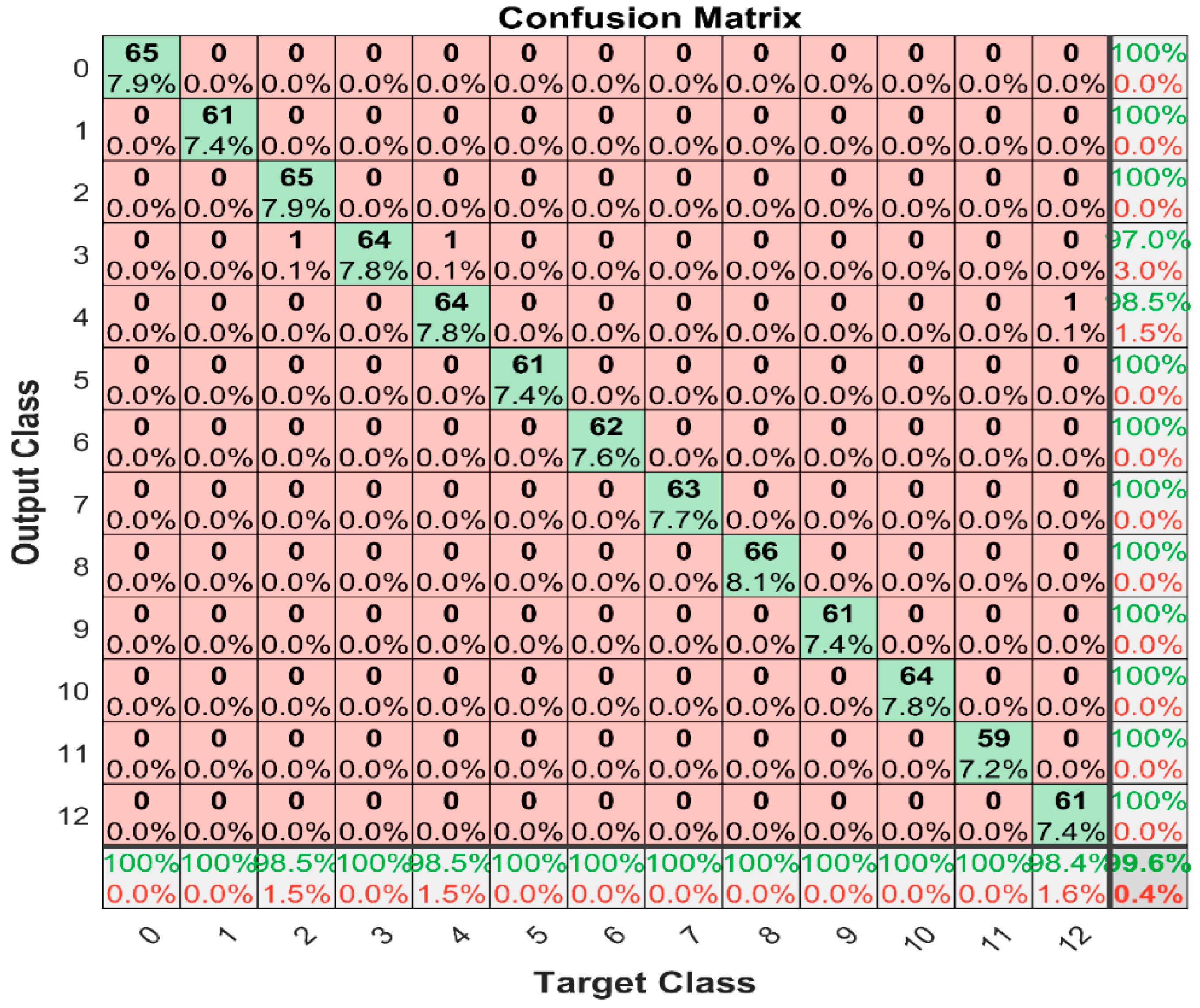
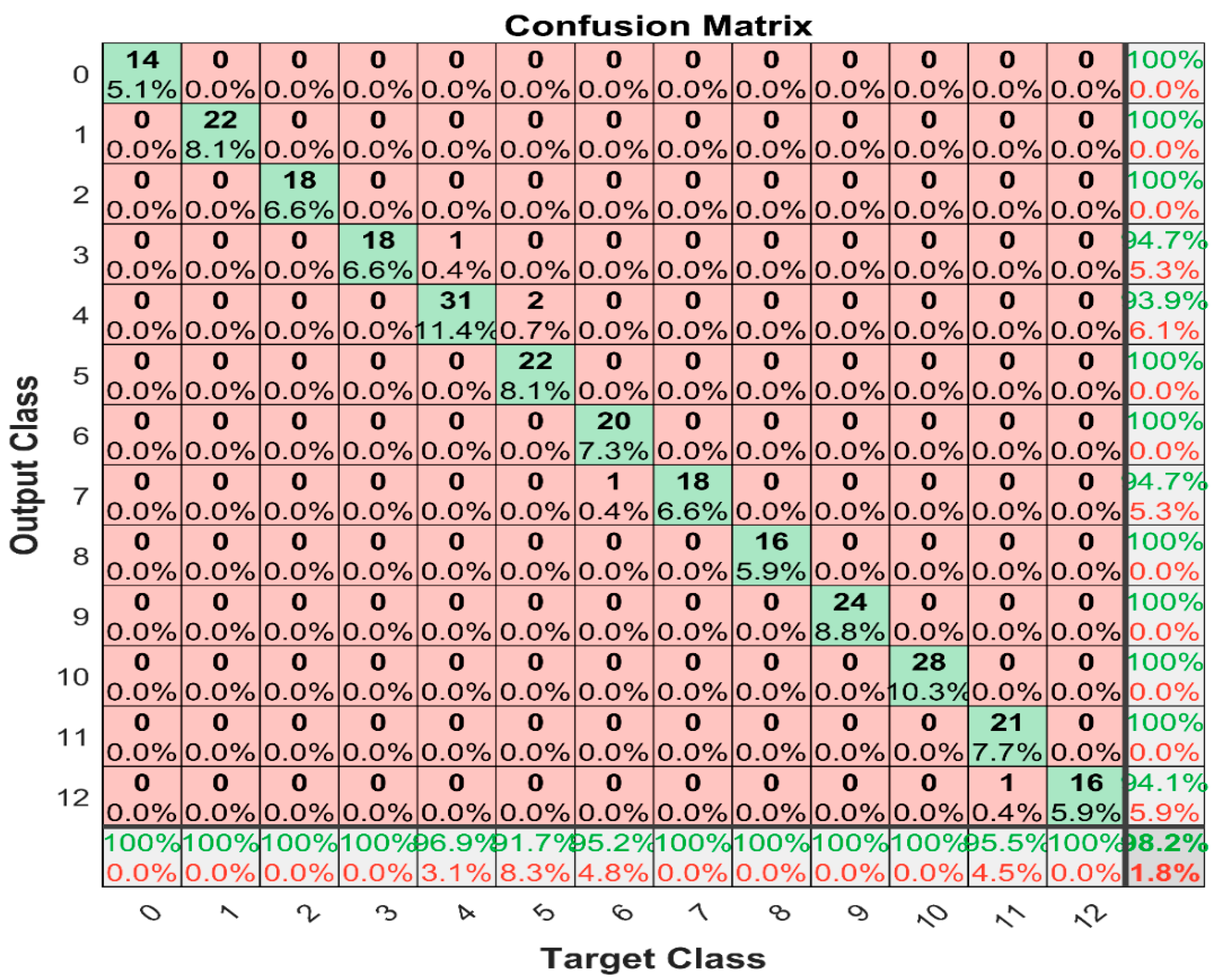
3.7.1. Single Fault Detection and Isolation

The fault detection and isolation accuracies of different techniques at 100% load operation were developed and presented in

Table 5. All algorithm family’s fault detection and isolation accuracy: Single fault at 100% load.

Candidate Algorithms	Accuracy [%]	Rank
Narrow Neural Network	98.62	1
Cubic Support Vector Machine	98.44	2
Tri-layered Neural Network	97.89	3
Wide Neural Network	97.80	4
Bi-layered Neural Network	97.80	5
Medium Neural Network	97.71	6
Fine KNN	97.06	7
Quadratic SVM	96.88	8
Weighted KNN	96.79	9
Bagged Trees	96.70	10
Fine Gaussian SVM	95.60	11
Subspace KNN	95.14	12
Linear SVM	93.95	13
Boosted Trees Ensemble	93.77	14
Medium Gaussian SVM	93.68	15
Medium KNN	93.68	16
Cubic KNN	93.40	17
SVM Kernel	93.40	18
Cosine KNN	92.94	19
Fine Tree	92.85	20
Logistic Regression Kernel	89.37	21
Coarse Gaussian SVM	83.79	22
RUSBoosted Trees	82.60	23
Medium Tree	82.50	24
Subspace Discriminant	81.59	25
Kernel naïve bays	79.76	26
Coarse KNN	72.25	27
Coarse Tree	35.80	28

. During development, the diagnostics model utilized data generated when the engine model was running at full load/100% load. The objective was to detect and isolate faults occurring during 100% load operation. Compared to other candidate techniques, the narrow neural network exhibits superior performance in accurately detecting and isolating single faults at full-load operation.

The narrow neural network outperformed better shown in

Table 6. Selected algorithm used as reference for further use and investigation: Single fault at 100% load.

Algorithms Type	Accuracy [%]	Rank
Narrow Neural Network	98.62	1

was taken as reference for further investigation to improve the network’s performance. This investigation involved simulating the model with different numbers of hidden layer neurons within a range of 5 to 19. Through this process, it was discovered that setting the network with 11 hidden layer neurons led to superior fault detection and isolation accuracy, particularly for single faults occurring at 100% load condition. In Figure 5, the number of neurons in the hidden layer versus the accuracy of single fault detection and isolation is shown, specifically focusing on the 100% load condition. This graph provides a comprehensive understanding of how the accuracy of fault detection and isolation fluctuates as the number of hidden layer neurons is adjusted. Figure 6 illustrates the network architecture with the inclusion of the 11 hidden layer neurons. The performance of the network was evaluated through training and validation, with the accuracy results depicted in Figure 7. Furthermore, the accuracy of the fault detection and isolation model was assessed using unseen or test data, and the results are presented in Figure 8.

Network training information that gave accurate prediction for single fault at 100% load:

• Pre-set Network: Neural Network
• Number of neurons in the hidden layer: 11
• Training Data Observation: 819 (75%)
• Testting Data Observation: 274 (25%)
• Training and Validation: 4-K-fold cross validation
• Training algorithm: Levenberg Marquardt
• Predictors variables: 10
• Response Classes: 13
• Activation function: Relu

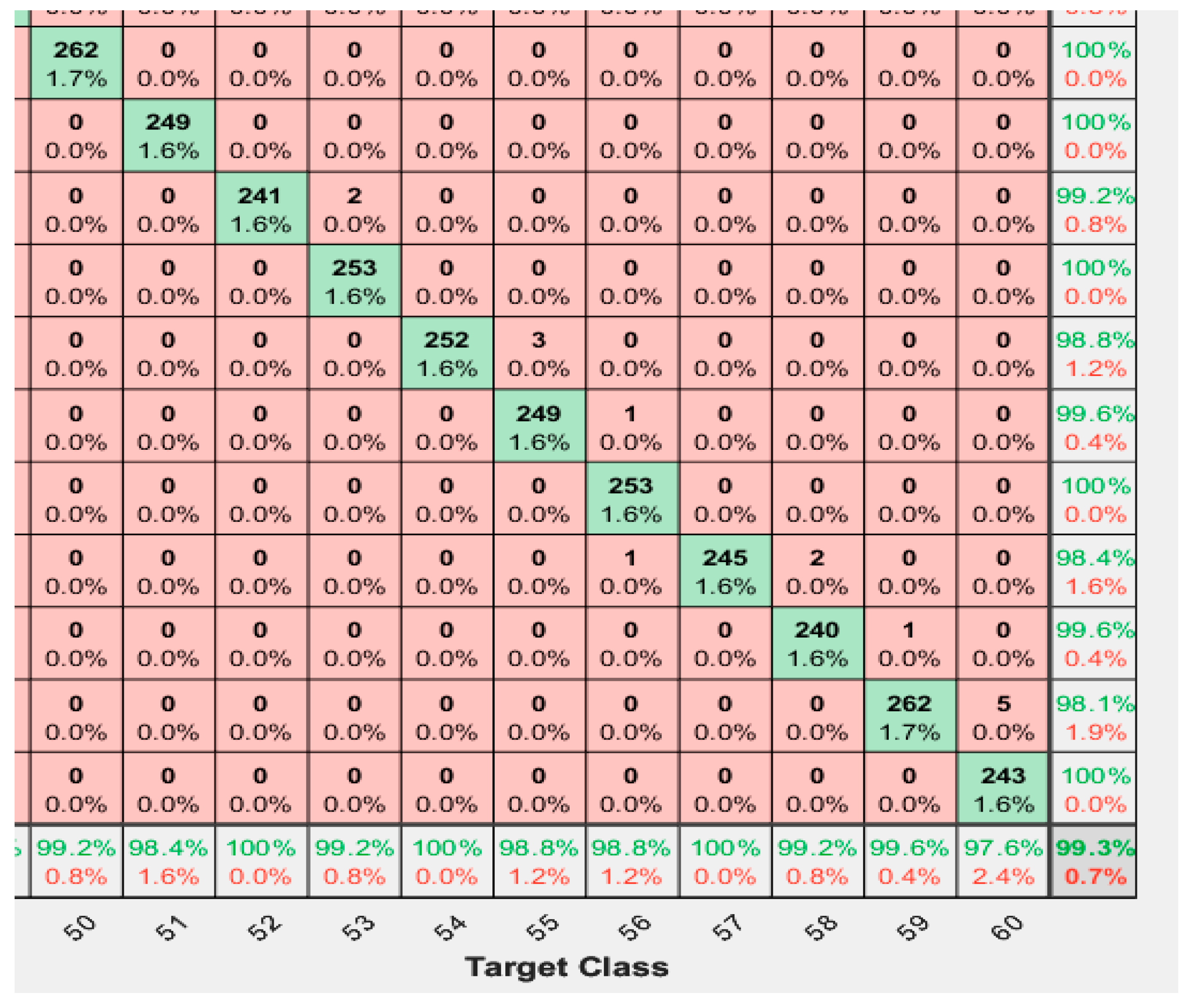
3.7.2. Double Fault Detection and Isolation

A double fault detection and isolation model was developed specifically to detect and isolate double faults that occur during 100% load conditions. To construct this model, data was collected by running the engine model at 100% load.

Table 7. All algorithm families fault detection and isolation accuracy: double fault at 100% load.

Candidate Algorithms	Accuracy [%]	Rank
Medium Neural Network	98.12	1
Wide Neural Network	97.31	2
Cubic SVM	97.27	3
Fine KNN	96.86	4
Bagged Trees	96.64	5
Quadratic SVM	96.27	6
Weighted KNN	96.25	7
Narrow Neural Network	94.41	8
Fine Gaussian SVM	93.96	9
Subspace KNN	93.94	10
Bilayered Neural Network	90.55	11
Cubic KNN	90.14	12
Medium KNN	90.06	13
Linear SVM	90.05	14
Cosine KNN	89.31	15
SVM Kernel	87.52	16
Medium Gaussian SVM	86.04	18
Trilayered Neural Network	79.92	19
Logistic Regression Kernel	75.46	20
Coarse Gaussian SVM	70.23	21
Coarse KNN	67.67	22
Kernel Naïve Bayes	61.99	23
Subspace Discriminant	58.20	24
Fine Tree	54.71	25
Boosted Trees	38.25	26
RUSBoosted Trees	27.29	27
Medium Tree	26.67	28
Coarse Tree	8.02	29

provides a comparison of the accuracy achieved by different techniques employed in the process. Upon comparing the various techniques employed, it becomes evident that the medium neural network again outperforms other methods in accurately detecting and isolating double faults when the engine operates under 100% load conditions.

Similarly, to enhance the performance of the medium neural network mentioned in

Table 8. Selected algorithm used as a reference for further investigation: double fault at 100% load.

Algorithms Type	Accuracy [%]	Rank
Medium Neural Network	98.12	1

and improve its accuracy, a further investigation was conducted. This investigation involved simulating the model with different numbers of hidden layer neurons, ranging from 20 to 34. Through this iterative process, it was found that setting the network with 28 hidden layer neurons resulted in the highest accuracy. This configuration proved to be most effective in accurately detecting and isolating double faults under full-load operation. Figure 9 provides the number of neurons in the hidden layer versus the accuracy of detecting and isolating double faults under a 100% load condition. To some extent, it demonstrates that, as the number of neurons in the hidden layer increases, the accuracy of fault detection and isolation improves. A visual representation of the network architecture with 28 hidden layer neurons is presented in Figure 10. The accuracy of the fault detection and isolation model, including training and validation, as well as testing with unseen data, is presented in Figure 11 and Figure 12. It shows the effectiveness of the model in accurately identifying and isolating faults.

Network training information that gave the best accuracy for double fault detection and isolation at 100% load:

• Machine learning technique: Neural Network
• Number of neurons in the hidden layer: 28
• Training Data Observation: 15,372 (75%)
• Testing Data Observation: 5124 (25%)
• Training and Validation: 4-K-fold cross-validation
• Predictors variables: 10
• Response Classes: 61
• Activation function: ReLU

In the same fashion, both single and double fault detection and isolation model has been developed when the engine load is at 80% and 90%, respectively. During development, the data generated when the engine operation was at 80% load and 90% load were used. This advanced model is designed to accurately identify and isolate potential faults that may occur during part-load operation, at 80% load and 90% load levels. It is, again, observed that neural networks outperform both single and double faults at 80% load and 90% load operation. For single fault isolation and detection at 80% and 90% load operation, the network was investigated within the range of hidden layer neuron numbers, from 5 to 19. While investigating the selected neural network model with changing the number of neurons within the range of neuron numbers, it is observed that setting the number of neurons at 15 resulted in improved fault detection and isolation accuracy for single faults at 80% load condition, and setting the number of neurons to 12 resulted in enhanced fault detection and isolation accuracy, specifically for single faults occurring at 90% load condition. The accuracy of the single fault detection and isolation model, including training and validation, as well as testing with unseen data, for both the 80% load and 90% load, is presented in Appendix B, Figure A1, Figure A2, Figure A3 and Figure A4.

For double fault isolation and detection at 80% load and 90% load, the neural network investigation involved simulating the model with varying numbers of hidden layer neurons, ranging from 20 to 34. By carrying out this process, it was discovered that setting the network with 32 hidden layer neurons resulted in superior accuracy for detecting and isolating double faults at 80% load condition, and setting the network with 30 hidden layer neurons resulted in superior accuracy for detecting and isolating double faults at 80% load condition. The accuracy of the double fault detection and isolation model, including training and validation, as well as testing with unseen data, for both 80% load and 90% load, is presented in Appendix C, Figure A5, Figure A6, Figure A7 and Figure A8.

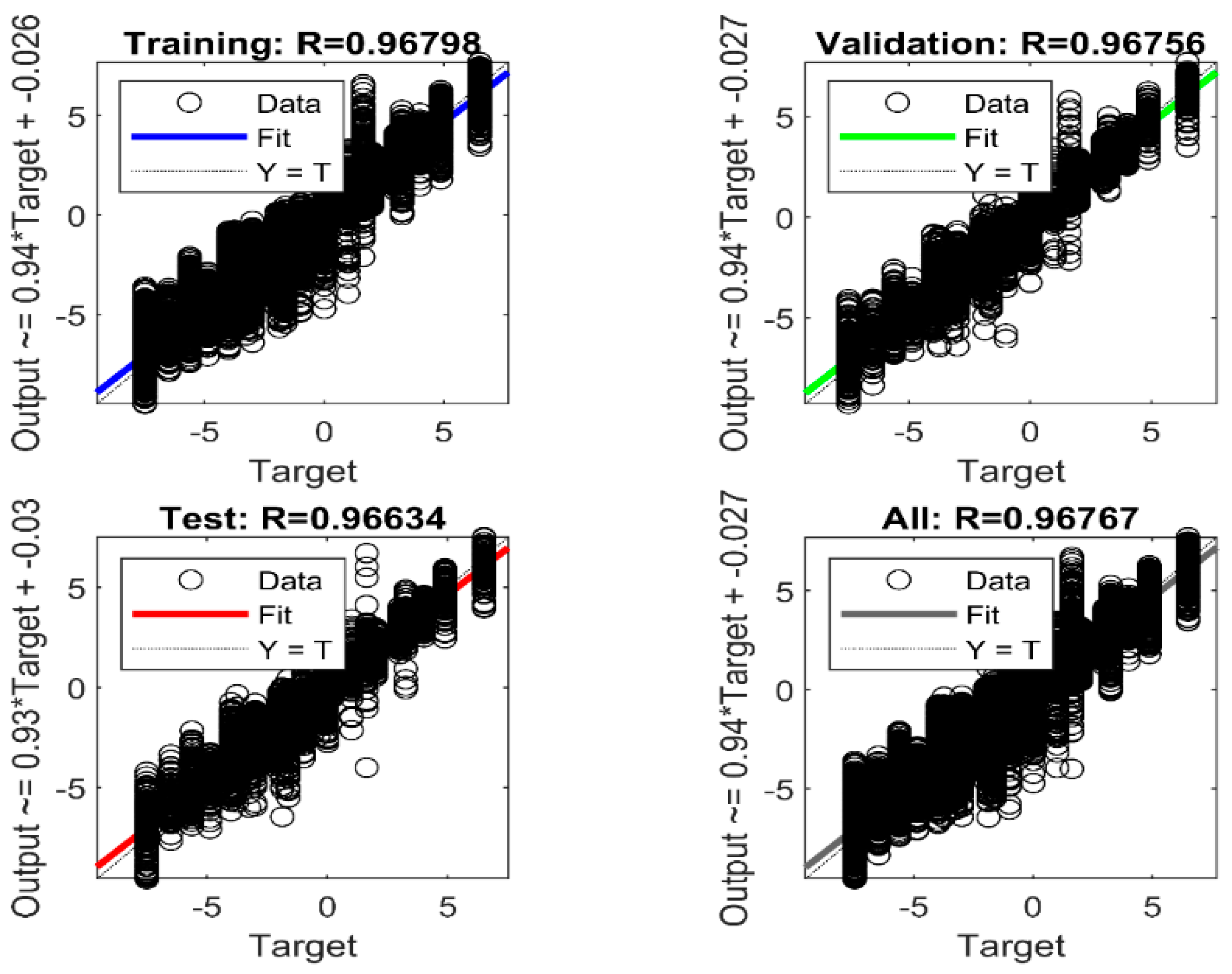
3.8. Fault Identification Model Results

Gas-path fault identification is a process that aims to estimate or quantify of a gas turbine’s component deterioration. The gas-path measurements, including temperature, pressure, spool speed, and fuel flow, are utilized as inputs or predictors for a fault identification network, which employs them to predict the health parameters of the engine, such as flow capacity, isentropic efficiency, and drift angle. In the context of this particular research, a significant focus was placed on VIGV (Variable Inlet Guide Vane) drift; thus, drift angle was employed as an additional response parameter. Because of its promising effectiveness, shown in the fault isolation and detection task, neural networks were chosen for the fault identification task. To improve fault identification accuracy, the hyperparameters were manipulated. For each of the single and double fault identifications at 80% load, 90% load, and 100% load, the network was simulated with different numbers of hidden layer neurons, ranging from 5 to 25, to identify what number of neurons should be in the hidden layer number for improved accuracy. The single and double fault identification pattern is presented in Appendix D,

Table A3. The input/predictors and output/responses parameters for single faults identification model.

NO	Fault Description	Predictor	Response
1	Clean	P24 T24 P3 T3 P43 P47 T5 FF N1 N2	All components $\Delta \eta$ $\& \Delta \Gamma$ are zero
2	LPC Fouling		$\Delta {\eta }_{LPC}$ $\& \Delta {\Gamma }_{LPC}$
3	HPC Fouling		$\Delta {\eta }_{HPC}$$\& \Delta {\Gamma }_{HPC}$
4	HPT Fouling		$\Delta {\eta }_{HPT}$$\& \Delta {\Gamma }_{HPT}$
5	LPT Fouling		$\Delta {\eta }_{LPT}$$\& \Delta {\Gamma }_{LPT}$
6	PT Fouling		$\Delta {\eta }_{PT}$$\& \Delta {\Gamma }_{PT}$
7	LPC Erosion		$\Delta {\eta }_{LPC}$$\& \Delta {\Gamma }_{LPC}$
8	HPC Erosion		$\Delta {\eta }_{HPC}$$\& \Delta {\Gamma }_{HPC}$
9	HPT Erosion		$\Delta {\eta }_{HPT}$$\& \Delta {\Gamma }_{HPT}$
10	LPT Erosion		$\Delta {\eta }_{LPT}$$\& \Delta {\Gamma }_{LPT}$
11	PT Erosion		$\Delta {\eta }_{PT}$$\& \Delta {\Gamma }_{PT}$
12	VIGV Updrift		$VIGVUPDRIFT$
13	VIGV Downdrift		$VIGVDOWNDRIFT$

and

Table A4. The input/predictors and output/responses parameters for double faults identification model.

NO	Fault Description	Predictor	Response
1	Clean	P24 T24 P3 T3 P43 P47 T5 FF N1 N2	All components $\Delta \eta$$\& \Delta \Gamma$ are zero
2	LPC Fouling & HPC Fouling		${\eta }_{LPC}$$, \Delta {\Gamma }_{LPC}$$, \Delta {\eta }_{HPC}$$\& \Delta {\Gamma }_{HPC}$
3	LPC Fouling & HPC Erosion
4	LPC Erosion & HPC Fouling
5	LPC Erosion & HPC Erosion
6	LPC Fouling & HPT Fouling		${\eta }_{LPC}$$, \Delta {\Gamma }_{LPC}$$, \Delta {\eta }_{HPT}$$\& \Delta {\Gamma }_{HPT}$
7	LPC Fouling & HPT Erosion
8	LPC Erosion & HPT Fouling
9	LPC Erosion & HPT Erosion
10	LPC Fouling & LPT Fouling		${\eta }_{LPC}$$, \Delta {\Gamma }_{LPC}$$, \Delta {\eta }_{LPT}$$\& \Delta {\Gamma }_{LPT}$
11	LPC Fouling & LPT Erosion
12	LPC Erosion & LPT Fouling
13	LPC Erosion & LPT Erosion
14	LPC Fouling & PT Fouling		${\eta }_{LPC}$$, \Delta {\Gamma }_{LPC}$$, \Delta {\eta }_{PT}$$\& \Delta {\Gamma }_{PT}$
15	LPC Fouling & PT Erosion
16	LPC Erosion & PT Fouling
17	LPC Erosion & PT Erosion
18	HPC Fouling & HPT Fouling		${\eta }_{HPC}$$, \Delta {\Gamma }_{HPC}$$, \Delta {\eta }_{HPT}$$\& \Delta {\Gamma }_{HPT}$
19	HPC Fouling & HPT Erosion
20	HPC Erosion & HPT Fouling
21	HPC Erosion & HPT Erosion
22	HPC Fouling & LPT Fouling		${\eta }_{HPC}$$, \Delta {\Gamma }_{HPC}$$, \Delta {\eta }_{LPT}$$\& \Delta {\Gamma }_{LPT}$
23	HPC Fouling & LPT Erosion
24	HPC Erosion & LPT Fouling
25	HPC Erosion & LPT Erosion
26	HPC Fouling & PT Fouling		${\eta }_{HPC}$$, \Delta {\Gamma }_{HPC}$$, \Delta {\eta }_{PT}$$\& \Delta {\Gamma }_{PT}$
27	HPC Fouling & PT Erosion
28	HPC Erosion & PT Fouling
29	HPC Erosion & PT Erosion
30	HPT Fouling & LPT Fouling		${\eta }_{HPT}$$, \Delta {\Gamma }_{HPT}$$, \Delta {\eta }_{LPT}$$\& \Delta {\Gamma }_{LPT}$
31	HPT Fouling & LPT Erosion
32	HPT Erosion & LPT Fouling
33	HPT Erosion & LPT Erosion
34	HPT Fouling & PT Fouling		${\eta }_{HPT}$$, \Delta {\Gamma }_{HPT}$$, \Delta {\eta }_{PT}$$\& \Delta {\Gamma }_{PT}$
35	HPT Fouling & PT Erosion
36	HPT Erosion & PT Fouling
37	HPT Erosion & PT Erosion
38	LPT Fouling & PT Fouling		${\eta }_{LPT}$$, \Delta {\Gamma }_{LPT}$$, \Delta {\eta }_{PT}$$\& \Delta {\Gamma }_{PT}$
39	LPT Fouling & PT Erosion
40	LPT Erosion & PT Fouling
41	LPT Erosion & PT Erosion
42	LPC Fouling & VIGV Updrift		${\eta }_{LPC}$$, \Delta {\Gamma }_{LPC}$$, VIGVUPDRIFT$
43	HPC Fouling & VIGV Updrift		${\eta }_{HPC}$$, \Delta {\Gamma }_{HPC}$$, VIGVUPDRIFT$
44	HPT Fouling & VIGV Updrift		${\eta }_{HPT}$$, \Delta {\Gamma }_{HPT}$$, VIGVUPDRIFT$
45	LPT Fouling & VIGV Updrift		${\eta }_{LPT}$$, \Delta {\Gamma }_{LPT}$$, VIGVUPDRIFT$
46	PT Fouling & VIGV Updrift		${\eta }_{PT}$$, \Delta {\Gamma }_{PT}$$, VIGVUPDRIFT$
47	LPC Fouling & VIGV Downdrift		${\eta }_{LPC}$$, \Delta {\Gamma }_{LPC}$$, VIGVDOWNDRIFT$
48	HPC Fouling & VIGV Downdrift		${\eta }_{HPC}$$, \Delta {\Gamma }_{HPC}$$, VIGVDOWNDRIFT$
49	HPT Fouling & VIGV Downdrift		${\eta }_{HPT}$$, \Delta {\Gamma }_{HPT}$$, VIGVDOWNDRIFT$
50	LPT Fouling & VIGV Downdrift		${\eta }_{LPT}$$, \Delta {\Gamma }_{LPT}$$, VIGVDOWNDRIFT$
51	PT Fouling & VIGV Downdrift		${\eta }_{PT}$$, \Delta {\Gamma }_{PT}$$, VIGVDOWNDRIFT$
52	LPC Erosion & VIGV Updrift		${\eta }_{LPC}$$, \Delta {\Gamma }_{LPC}$$, VIGVUPDRIFT$
53	HPC Erosion & VIGV Updrift		${\eta }_{HPC}$$, \Delta {\Gamma }_{HPC}$$, VIGVUPDRIFT$
54	HPT Erosion & VIGV Updrift		${\eta }_{HPT}$$, \Delta {\Gamma }_{HPT}$$, VIGVUPDRIFT$
55	LPT Erosion & VIGV Updrift		${\eta }_{LPT}$$, \Delta {\Gamma }_{LPT}$$, VIGVUPDRIFT$
56	PT Erosion & VIGV Updrift		${\eta }_{PT}$$, \Delta {\Gamma }_{PT}$$, VIGVUPDRIFT$
57	LPC Erosion & VIGV Downdrift		${\eta }_{LPC}$$, \Delta {\Gamma }_{LPC}$$, VIGVDOWNDRIFT$
58	HPC Erosion & VIGV Downdrift		${\eta }_{HPC}$$, \Delta {\Gamma }_{HPC}$$, VIGVDOWNDRIFT$
59	HPT Erosion & VIGV Downdrift		${\eta }_{HPT}$$, \Delta {\Gamma }_{HPT}$$, VIGVDOWNDRIFT$
60	LPT Erosion & VIGV Downdrift		${\eta }_{LPT}$$, \Delta {\Gamma }_{LPT}$$, VIGVDOWNDRIFT$
61	PT Erosion & VIGV Downdrift		${\eta }_{PT}$$, \Delta {\Gamma }_{PT}$$, VIGVDOWNDRIFT$

.

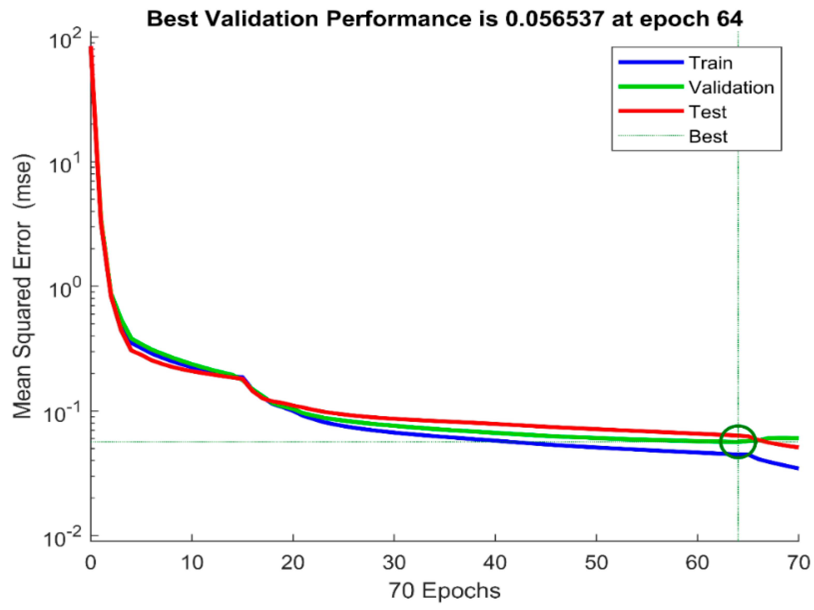
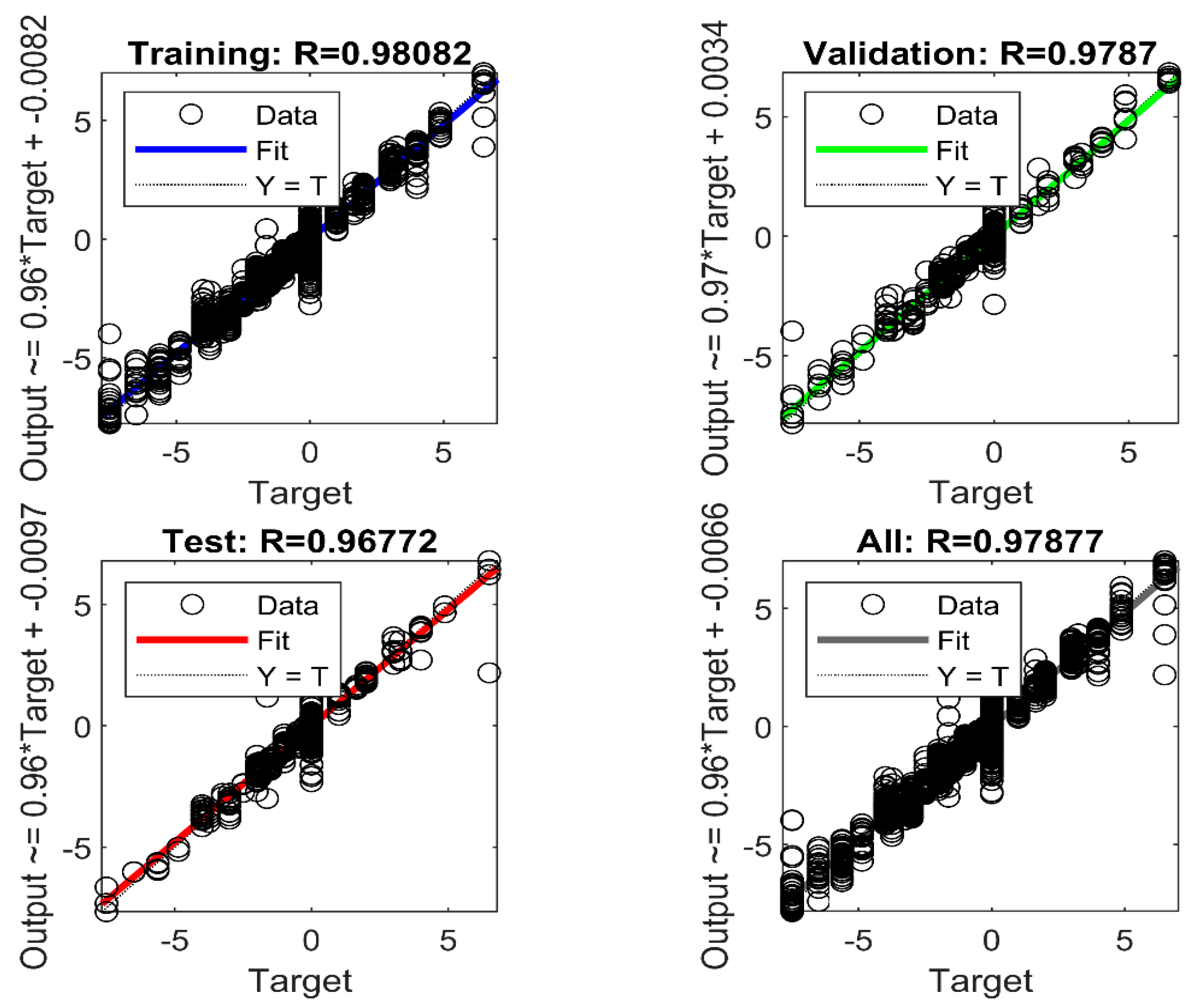
3.8.1. Single Fault Identification at 100% Load

In the same fashion, through an iterative process, it was determined that the network achieved the highest accuracy when the number of neurons in the hidden layer was set to 17. Figure 13 provides a visual representation of the model’s optimal performance in terms of validation. In this configuration, the mean square error was calculated to be 0.156 at 209 epochs. Figure 14 shows the single fault identification at 100% load model accuracy.

Network training information that gave accurate prediction for single fault identification at 100% load:

• Pre-set Network: Neural Network
• Number of Neurons in the Hidden Layer: 17
• Training Data Observation: 765
• Validation Data Observation: 164
• Test Data Observation: 164
• Training Algorithm: Levenberg Marquardt
• Predictors Variables: 10
• Response Classes: 11
• Activation Function: ReLU
• Performance: Mean Square Error
• Data Division: Random

3.8.2. Double Fault Identification at 100% Load

To assess the accuracy of the model, simulations were conducted by varying the number of neurons in the hidden layer, ranging from 5 to 25. Through iteration of this process, it was found that the network achieved the highest accuracy when the number of neurons in the hidden layer was set to 21. Figure 15 illustrates the optimal performance of the model in terms of validation. In this configuration, the mean square error was calculated to be 0.176 at 391 epochs. Figure 16 shows the double fault identification at 100% load model accuracy.

Network training information that gave accurate prediction for double fault identification at 100% load:

• Pre-set Network: Neural Network
• Number of Neurons in the Hidden Layer: 21
• Training Data Observation: 14,346
• Validation Data Observation: 3075
• Test Data Observation: 3075
• Training Algorithm: Levenberg Marquardt
• Predictors Variables: 10
• Response Classes: 11
• Activation Function: ReLU
• Performance: Mean Square Error
• Data Division: Random

In the same fashion, both single and double fault identification models were developed when the engine load was at 80% and 90%. Because of its promising accuracy, shown in the fault detection and isolation accuracy, neural network used fault identification tasks at different loads. Through the iterative process of hidden layer neurons, it was found that setting the network with 20 hidden layer neurons resulted in the highest accuracy for single fault identification at 80% load. The mean square error is 0.029, and the epoch is 152. For fault identification at 90% load, it was found that setting the network with 19 hidden layer neurons resulted in the highest accuracy. The mean square error is 0.056 at 64 epochs. The single fault identification neural network model at 80% load and 90% load results are presented in Appendix E, Figure A9, Figure A10, Figure A11 and Figure A12. To investigate the double fault identification at 80% load and 90% load, simulations were conducted with varying numbers of hidden layer neurons, ranging from 5 to 25. Again, through an iterative process, it was determined that the double fault identification at 80% load network achieved the highest accuracy when the number of neurons in the hidden layer was set to 25, while the double fault identification at 90% load network achieved the highest accuracy when the number of neurons in the hidden layer was set to 23. The mean square error of the double fault identification at 80% load network is calculated to be 0.154, and the training process stopped at 259 epochs, while the mean square error of the double fault identification at 90% load network is calculated to be 0.156, and the training process stopped at 209 epochs. The double fault identification neural network model at 80% load and 90% load results are presented in Appendix F, Figure A13, Figure A14, Figure A15 and Figure A16. The summary of the faults isolation and isolation accuracy presented in

Table 9. Single and double faults detection and isolation model accuracy at different loads summary.

	Single Faults Detection and Isolation			Double Faults Detection and Isolation
	80% Load	90% Load	100% Load	80% Load	90% Load	100% Load
Validation accuracy	99.6%	99.8%	99.8%	99.4%	99.3%	99.5%
Test accuracy	98.9%	98.2%	98.9%	98.7%	98.4%	98.1%

, and the summary of the fault identification accuracy presented in

Table 10. Single and double faults identification model accuracy at different loads summary.

	Single Faults Detection and Isolation			Double Faults Detection and Isolation
	80% Load	90% Load	100% Load	80% Load	90% Load	100% Load
Training accuracy	99.14%	98.08%	96..79%	96.86%	96.79%	96.35%
Validation accuracy	98.88%	97.87%	96.75%	96.82%	96.75%	96.31%
Test accuracy	97.67%	96.77%	96.63%	96.74%	96.63%	95.98%
All accuracy	98.86%	97.87%	96.76%	96.83%	96.76%	96.28%

.

3.9. Comparison of Diagnostics Results with Available Literature

One way to assess the effectiveness of a newly proposed diagnostic method is by conducting a direct comparison with existing methods. This approach involves evaluating the diagnostic performance of the new method relative to others. However, it is important to ensure that the methods being compared have specifically addressed similar gas turbine problems with the same configurations and levels of complexity [93]. By doing so, a fair and meaningful evaluation can be carried out. Therefore, to compare the diagnostics model accuracy, one of the latest three-shaft gas turbine diagnostic models were found and used for comparison. Mingliang et al. [94] have developed the diagnostics model. The have considered 13 single faults, while double faults remained unconsidered. The have considered fouling and foreign object damage in the compressors and fouling, erosion, and foreign object damage in the turbines. They did not consider erosion in the compressors. The model that they developed is only for fault detection and isolation at full-load; fault identification tasks and part-load operations are not considered in their study. Even though there is a difference on considering the type of physical faults in the fault detection and isolation, their study is used for comparison because of the similarity of the engine configuration and the number of single faults considered. The fault detection and isolation accuracy of their model and our model at full load is 99.3% and 89.9%, respectively. The comparison shows that the diagnosis model proposed in this research has a promising accuracy. Furthermore, in this research, both single and double faults at full- and part-load operations are considered, which made the developed diagnostics model comprehensive.

4. Conclusions

The results shows that the neural network group demonstrated high detection and isolation accuracy for single faults at each load condition. The fault detection and isolation model’s accuracy is higher than the fault identification model’s accuracy. Because the number of double faults considered are greater than the number of single faults, the detection and isolation accuracy of single faults are greater than the accuracy of double faults detection and isolation models at each load. However, the fault detection and isolation model accuracy achieved for all three load conditions were between 99.3% and 99.5% for the training and validation, and between 98.1% and 98.7% for the test data. The single and double fault identification model accuracies for all the three load conditions ranges between 96% and 99%. Even though the computation time does not matter that much, as there are high-performance computers, the increase of hidden layer neurons causes the computation time to increase. A comprehensive investigation has been done, and the results indicate that the developed neural network models exhibit high accuracy in fault detection, isolation, and identification tasks, suggesting their effectiveness in diagnosing faults in the gas turbine system.

References

1. Benini, E. Progress in Gas Turbine Performance; BoD–Books on Demand: Holstein, Germany, 2013. [Google Scholar]
2. Meher-Homji, C.B.; Chaker, M.A.; Motiwala, H.M. Gas Turbine Performance Deterioration. In Proceedings of the 30th Turbomachinery Symposium, College Station, TX, USA, 30 September–3 October 2001; Texas A&M University, Turbomachinery Laboratories: College Station, TX, USA, 2001. [Google Scholar]
3. Meher-Homji, C.B.; Matthews, T.; Pelagotti, A.; Weyermann, H.P. Gas Turbines And Turbocompressors For LNG Service. In Proceedings of the 36th Turbomachinery Symposium, College Station, TX, USA, 2 August 2007; Texas A&M University, Turbomachinery Laboratories: College Station, TX, USA, 2007. [Google Scholar]
4. Marinai, L.; Singh, R.; Curnock, B.; Probert, D. Detection and prediction of the performance deterioration of a turbofan engine. In Proceedings of the International Gas Turbine Congress, Tokyo, Japan, 2–7 November 2003; pp. 2–7. [Google Scholar]
5. Diakunchak, I.S. Performance deterioration in industrial gas turbines. J. Eng. Gas Turbines Power 1992, 114, 161–168. [Google Scholar] [CrossRef]
6. Melino, F.; Morini, M.; Peretto, A.; Pinelli, M.; Ruggero Spina, P. Compressor fouling modeling: Relationship between computational roughness and gas turbine operation time. J. Eng. Gas Turbines Power 2012, 134, 052401. [Google Scholar] [CrossRef]
7. Meher-Homji, C.B.; Chaker, M.; Bromley, A.F. The fouling of axial flow compressors: Causes, effects, susceptibility, and sensitivity. In Turbo Expo: Power for Land, Sea, and Air; American Society of Mechanical Engineers: New York, NY, USA, 2009; Volume 48852, pp. 571–590. [Google Scholar]
8. Morini, M.; Pinelli, M.; Spina, P.R.; Venturini, M. Influence of blade deterioration on compressor and turbine performance. J. Eng. Gas Turbines Power 2010, 132, 032401. [Google Scholar] [CrossRef]
9. Giampaolo, T. The Gas Turbine Handbook: Principles and Practices; Prentice Hall: Hoboken, NJ, USA, 1997. [Google Scholar]
10. Cruz-Manzo, S.; Panov, V.; Zhang, Y. Gas path fault and degradation modelling in twin-shaft gas turbines. Machines 2018, 6, 43. [Google Scholar] [CrossRef]
11. Suman, A.; Casari, N.; Fabbri, E.; Pinelli, M.; di Mare, L.; Montomoli, F. Gas turbine fouling tests: Review, critical analysis, and particle impact behavior map. J. Eng. Gas Turbines Power 2019, 141, 4041282. [Google Scholar] [CrossRef]
12. Hashmi, M.B.; Abd Majid, M.A.; Lemma, T.A. Combined effect of inlet air cooling and fouling on performance of variable geometry industrial gas turbines. Alex. Eng. J. 2020, 59, 1811–1821. [Google Scholar] [CrossRef]
13. Madsen, S.; Bakken, L.E. Gas turbine fouling offshore: Effective online water wash through high water-to-air ratio. In Turbo Expo: Power for Land, Sea, and Air; American Society of Mechanical Engineers: New York, NY, USA, 2018; Volume 51180, p. V009T027A016. [Google Scholar]
14. Herdzik, J. Dependence between nominal power deterioration and thermal efficiency of gas turbines due to fouling. Sci. J. Marit. Univ. Szczec. 2022, 69, 45–53. [Google Scholar]
15. Diakunchak, I.S. Performance Deterioration in Industrial Gas Turbines; Citeseer: Princeton, NJ, USA, 1991; Volume 79016. [Google Scholar]
16. Varelis, A.G. Technoeconomic Study of Engine Deterioration and Compressor Washing for Military Gas Turbine Engines; Cranfield University: Bedford, UK, 2008. [Google Scholar]
17. Abdi, F.; Eftekharian, A.; Huang, D.; Choi, S.; Morscher, G.N.; Panakarajupally, R.P. ICME Modeling of Erosion in Gas-Turbine Grade CMC and HVOF Test. In Turbo Expo: Power for Land, Sea, and Air; American Society of Mechanical Engineers: New York, NY, USA, 2022; Volume 85970, p. V001T002A009. [Google Scholar]
18. Salilew, W.M.; Abdul Karim, Z.A.; Lemma, T.A.; Fentaye, A.D.; Kyprianidis, K.G. The Effect of Physical Faults on a Three-Shaft Gas Turbine Performance at Full-and Part-Load Operation. Sensors 2022, 22, 7150. [Google Scholar] [CrossRef]
19. Kurz, R.; Brun, K. Gas Turbine Tutorial-Maintenance And Operating Practices Effects On Degradation And Life. In Proceedings of the 36th Turbomachinery Symposium, College Station, TX, USA, 2 August 2007; Texas A&M University, Turbomachinery Laboratories: College Station, TX, USA, 2007. [Google Scholar]
20. Muthuraman, S.; Twiddle, J.; Singh, M.; Connolly, N. Condition monitoring of SSE gas turbines using artificial neural networks. Insight-Non-Destr. Test. Cond. Monit. 2012, 54, 436–439. [Google Scholar] [CrossRef]
21. Kurz, R.; Brun, K. Degradation of gas turbine performance in natural gas service. J. Nat. Gas Sci. Eng. 2009, 1, 95–102. [Google Scholar] [CrossRef]
22. Diakunchak, I.S. Performance improvement in industrial gas turbines. In Turbo Expo: Power for Land, Sea, and Air; American Society of Mechanical Engineers: New York, NY, USA, 1993; Volume 79092, p. V001T001A005. [Google Scholar]
23. Kurz, R.; Brun, K.; Wollie, M. Degradation effects on industrial gas turbines. J. Eng. Gas Turbines Power 2009, 131, 062401. [Google Scholar] [CrossRef]
24. Zwebek, A. Combined Cycle Performance Deterioration Analysis. Ph.D. Thesis, Cranfield University, Cranfield, UK, 2002. [Google Scholar]
25. Jasmani, M.S.; Li, Y.-G.; Ariffin, Z. Measurement Selections for Multi-Component Gas Path Diagnostics Using Analytical Approach and Measurement Subset Concept. In Turbo Expo: Power for Land, Sea, and Air; American Society of Mechanical Engineers: New York, NY, USA, 2010; Volume 43987, pp. 569–579. [Google Scholar]
26. Chapman, J.W.; Lavelle, T.M.; Litt, J.S. Practical techniques for modeling gas turbine engine performance. In Proceedings of the 52nd AIAA/SAE/ASEE Joint Propulsion Conference, Salt Lake City, UT, USA, 25–27 July 2016; p. 4527. [Google Scholar]
27. Razak, A. Gas turbine performance modelling, analysis and optimisation. In Modern Gas Turbine Systems; Elsevier: Amsterdam, The Netherlands, 2013; pp. 423–514. [Google Scholar]
28. Ahmad, N. Numerical Modeling and Analysis of Small Gas Turbine Engine: Part I: Analytical Model and Compressor CFD. Master’s Thesis, Royal Institute of Technology, Stockholm, Sweden, 2009. [Google Scholar]
29. Zhong, S.-s.; Fu, S.; Lin, L. A novel gas turbine fault diagnosis method based on transfer learning with CNN. Measurement 2019, 137, 435–453. [Google Scholar] [CrossRef]
30. Kamarzarrin, M.; Refan, M.H.; Amiri, P.; Dameshghi, A. A new intelligent fault diagnosis and prognosis method for wind turbine doubly-fed induction generator. Wind Eng. 2022, 46, 308–340. [Google Scholar] [CrossRef]
31. Zhou, D.; Yao, Q.; Wu, H.; Ma, S.; Zhang, H. Fault diagnosis of gas turbine based on partly interpretable convolutional neural networks. Energy 2020, 200, 117467. [Google Scholar] [CrossRef]
32. Li, W.; Huang, R.; Li, J.; Liao, Y.; Chen, Z.; He, G.; Yan, R.; Gryllias, K. A perspective survey on deep transfer learning for fault diagnosis in industrial scenarios: Theories, applications and challenges. Mech. Syst. Signal Process. 2022, 167, 108487. [Google Scholar] [CrossRef]
33. Li, J.; Ying, Y. Gas turbine gas path diagnosis under transient operating conditions: A steady state performance model based local optimization approach. Appl. Therm. Eng. 2020, 170, 115025. [Google Scholar] [CrossRef]
34. Fast, M.; Assadi, M.; De, S. Development and multi-utility of an ANN model for an industrial gas turbine. Appl. Energy 2009, 86, 9–17. [Google Scholar] [CrossRef]
35. Fentaye, A.D.; Baheta, A.T.; Gilani, S.I.; Kyprianidis, K.G. A review on gas turbine gas-path diagnostics: State-of-the-art methods, challenges and opportunities. Aerospace 2019, 6, 83. [Google Scholar] [CrossRef]
36. Tahan, M.; Tsoutsanis, E.; Muhammad, M.; Karim, Z.A. Performance-based health monitoring, diagnostics and prognostics for condition-based maintenance of gas turbines: A review. Appl. Energy 2017, 198, 122–144. [Google Scholar] [CrossRef]
37. Salilew, W.M.; Karim, Z.A.A.; Lemma, T.A. Investigation of fault detection and isolation accuracy of different Machine learning techniques with different data processing methods for gas turbine. Alex. Eng. J. 2022, 61, 12635–12651. [Google Scholar] [CrossRef]
38. Barad, S.G.; Ramaiah, P.; Giridhar, R.; Krishnaiah, G. Neural network approach for a combined performance and mechanical health monitoring of a gas turbine engine. Mech. Syst. Signal Process. 2012, 27, 729–742. [Google Scholar] [CrossRef]
39. Fentaye, A.D.; Ul-Haq Gilani, S.I.; Baheta, A.T.; Li, Y.-G. Performance-based fault diagnosis of a gas turbine engine using an integrated support vector machine and artificial neural network method. Proc. Inst. Mech. Eng. Part A J. Power Energy 2019, 233, 786–802. [Google Scholar] [CrossRef]
40. Tahan, M.; Muhammad, M.; Abdul Karim, Z.A. A multi-nets ANN model for real-time performance-based automatic fault diagnosis of industrial gas turbine engines. J. Braz. Soc. Mech. Sci. Eng. 2017, 39, 2865–2876. [Google Scholar] [CrossRef]
41. Mathioudakis, K.; Kamboukos, P. Assessment of the effectiveness of gas path diagnostic schemes. J. Eng. Gas Turbines Power 2006, 128, 57–63. [Google Scholar] [CrossRef]
42. Hanachi, H.; Mechefske, C.; Liu, J.; Banerjee, A.; Chen, Y. Performance-based gas turbine health monitoring, diagnostics, and prognostics: A survey. IEEE Trans. Reliab. 2018, 67, 1340–1363. [Google Scholar] [CrossRef]
43. Kong, C. Review on advanced health monitoring methods for aero gas turbines using model based methods and artificial intelligent methods. Int. J. Aeronaut. Space Sci. 2014, 15, 123–137. [Google Scholar] [CrossRef]
44. Escher, P. Pythia: An Object-Orientated Gas Path Analysis Computer Program for General Applications. Ph.D. Thesis, Cranfield University, Cranfield, UK, 1995. [Google Scholar]
45. Fentaye, A.D.; Gilani, S.I.U.-H.; Baheta, A.T. Gas turbine gas path diagnostics: A review. In MATEC Web of Conferences; EDP Sciences: Les Ulis, France, 2016; Volume 74, p. 00005. [Google Scholar]
46. Chen, Y.-Z.; Zhao, X.-D.; Xiang, H.-C.; Tsoutsanis, E. A sequential model-based approach for gas turbine performance diagnostics. Energy 2021, 220, 119657. [Google Scholar] [CrossRef]
47. Lu, F.; Chen, Y.; Huang, J.; Zhang, D.; Liu, N. An integrated nonlinear model-based approach to gas turbine engine sensor fault diagnostics. Proc. Inst. Mech. Eng. Part G J. Aerosp. Eng. 2014, 228, 2007–2021. [Google Scholar] [CrossRef]
48. Kong, C.; Ki, J. Components map generation of gas turbine engine using genetic algorithms and engine performance deck data. J. Eng. Gas Turbines Power 2007, 129, 312–317. [Google Scholar] [CrossRef]
49. Li, Y.; Pilidis, P.; Newby, M. An adaptation approach for gas turbine design-point performance simulation. In Turbo Expo: Power for Land, Sea, and Air; American Society of Mechanical Engineers: New York, NY, USA, 2005; Volume 47284, pp. 95–105. [Google Scholar]
50. Kong, C.; Ki, J.; Kang, M. A new scaling method for component maps of gas turbine using system identification. J. Eng. Gas Turbines Power 2003, 125, 979–985. [Google Scholar] [CrossRef]
51. Marinai, L.; Probert, D.; Singh, R. Prospects for aero gas-turbine diagnostics: A review. Appl. Energy 2004, 79, 109–126. [Google Scholar] [CrossRef]
52. Li, Y. Performance-analysis-based gas turbine diagnostics: A review. Proc. Inst. Mech. Eng. Part A J. Power Energy 2002, 216, 363–377. [Google Scholar] [CrossRef]
53. Djaidir, B.; Hafaifa, A.; Kouzou, A. Vibration detection in gas turbine rotor using artificial neural network combined with continuous wavelet. In Advances in Acoustics and Vibration, Proceedings of the International Conference on Acoustics and Vibration (ICAV2016), Hammamet, Tunisia, 21–23 March 2016; Springer: Berlin/Heidelberg, Germany, 2016; pp. 101–113. [Google Scholar]
54. Talaat, M.; Gobran, M.; Wasfi, M. A hybrid model of an artificial neural network with thermodynamic model for system diagnosis of electrical power plant gas turbine. Eng. Appl. Artif. Intell. 2018, 68, 222–235. [Google Scholar] [CrossRef]
55. Soomro, A.A.; Mokhtar, A.A.; Salilew, W.M.; Abdul Karim, Z.A.; Abbasi, A.; Lashari, N.; Jameel, S.M. Machine Learning Approach to Predict the Performance of a Stratified Thermal Energy Storage Tank at a District Cooling Plant Using Sensor Data. Sensors 2022, 22, 7687. [Google Scholar] [CrossRef] [PubMed]
56. Soomro, A.A.; Mokhtar, A.A.; Kurnia, J.C.; Lashari, N.; Lu, H.; Sambo, C. Integrity assessment of corroded oil and gas pipelines using machine learning: A systematic review. Eng. Fail. Anal. 2022, 131, 105810. [Google Scholar] [CrossRef]
57. Sun, X.-L.; Wang, N. Gas turbine fault diagnosis using intuitionistic fuzzy fault Petri nets. J. Intell. Fuzzy Syst. 2018, 34, 3919–3927. [Google Scholar] [CrossRef]
58. Amare, F.; Gilani, S.; Aklilu, B.; Mojahid, A. Two-shaft stationary gas turbine engine gas path diagnostics using fuzzy logic. J. Mech. Sci. Technol. 2017, 31, 5593–5602. [Google Scholar] [CrossRef]
59. Yazdani, S.; Montazeri-Gh, M. A novel gas turbine fault detection and identification strategy based on hybrid dimensionality reduction and uncertain rule-based fuzzy logic. Comput. Ind. 2020, 115, 103131. [Google Scholar] [CrossRef]
60. Soomro, A.A.; Mokhtar, A.A.; Kurnia, J.C.; Lashari, N.; Sarwar, U.; Jameel, S.M.; Inayat, M.; Oladosu, T.L. A review on Bayesian modeling approach to quantify failure risk assessment of oil and gas pipelines due to corrosion. Int. J. Press. Vessel. Pip. 2022, 200, 104841. [Google Scholar] [CrossRef]
61. Mirhosseini, A.M.; Adib Nazari, S.; Maghsoud Pour, A.; Etemadi Haghighi, S.; Zareh, M. Probabilistic failure analysis of hot gas path in a heavy-duty gas turbine using Bayesian networks. Int. J. Syst. Assur. Eng. Manag. 2019, 10, 1173–1185. [Google Scholar] [CrossRef]
62. Zaccaria, V.; Rahman, M.; Aslanidou, I.; Kyprianidis, K. A review of information fusion methods for gas turbine diagnostics. Sustainability 2019, 11, 6202. [Google Scholar] [CrossRef]
63. Zaccaria, V.; Fentaye, A.D.; Kyprianidis, K. Assessment of dynamic Bayesian models for gas turbine diagnostics, Part 1: Prior probability analysis. Machines 2021, 9, 298. [Google Scholar] [CrossRef]
64. Luo, H.; Zhong, S. Gas turbine engine gas path anomaly detection using deep learning with Gaussian distribution. In Proceedings of the 2017 Prognostics and System Health Management Conference (PHM-Harbin), Harbin, China, 9–12 July 2017; IEEE: Piscataway, NJ, USA, 2017; pp. 1–6. [Google Scholar]
65. Mohtasham Khani, M.; Vahidnia, S.; Ghasemzadeh, L.; Ozturk, Y.E.; Yuvalaklioglu, M.; Akin, S.; Ure, N.K. Deep-learning-based crack detection with applications for the structural health monitoring of gas turbines. Struct. Health Monit. 2020, 19, 1440–1452. [Google Scholar] [CrossRef]
66. Yan, W.; Yu, L. On accurate and reliable anomaly detection for gas turbine combustors: A deep learning approach. arXiv 2019, arXiv:1908.09238. [Google Scholar]
67. Yan, W. Detecting gas turbine combustor anomalies using semi-supervised anomaly detection with deep representation learning. Cogn. Comput. 2020, 12, 398–411. [Google Scholar] [CrossRef]
68. Manservigi, L.; Murray, D.; de la Iglesia, J.A.; Ceschini, G.F.; Bechini, G.; Losi, E.; Venturini, M. Detection of Unit of Measure Inconsistency in gas turbine sensors by means of Support Vector Machine classifier. ISA Trans. 2022, 123, 323–338. [Google Scholar] [CrossRef]
69. Yan, L.; Cao, Y.; Liu, R.; Zhao, T.; Li, S. A Support Vector Machine Fault Diagnosis Method for Gas Turbine Fuel System. In Proceedings of the TEPEN 2022: Efficiency and Performance Engineering Network, Online, 18–21 August 2022; Springer: Berlin/Heidelberg, Germany, 2023; pp. 985–994. [Google Scholar]
70. Wang, H.; Peng, M.-j.; Hines, J.W.; Zheng, G.-y.; Liu, Y.-k.; Upadhyaya, B.R. A hybrid fault diagnosis methodology with support vector machine and improved particle swarm optimization for nuclear power plants. ISA Trans. 2019, 95, 358–371. [Google Scholar] [CrossRef]
71. Xi, P.-P.; Zhao, Y.-P.; Wang, P.-X.; Li, Z.-Q.; Pan, Y.-T.; Song, F.-Q. Least squares support vector machine for class imbalance learning and their applications to fault detection of aircraft engine. Aerosp. Sci. Technol. 2019, 84, 56–74. [Google Scholar] [CrossRef]
72. Aslinezhad, M.; Hejazi, M.A. Turbine blade tip clearance determination using microwave measurement and k-nearest neighbour classifier. Measurement 2020, 151, 107142. [Google Scholar] [CrossRef]
73. Naimi, A.; Deng, J.; Shimjith, S.; Arul, A.J. Fault detection and isolation of a pressurized water reactor based on neural network and k-nearest neighbor. IEEE Access 2022, 10, 17113–17121. [Google Scholar] [CrossRef]
74. Hadi, A.H.; Shareef, W.F. In-Situ Event Localization for Pipeline Monitoring System Based Wireless Sensor Network Using K-Nearest Neighbors and Support Vector Machine. J. Al-Qadisiyah Comput. Sci. Math. 2020, 12, 11–15. [Google Scholar]
75. Li, Y.-G. Diagnostics of power setting sensor fault of gas turbine engines using genetic algorithm. Aeronaut. J. 2017, 121, 1109–1130. [Google Scholar] [CrossRef]
76. Ahn, B.H.; Yu, H.T.; Choi, B.K. Feature-based analysis for fault diagnosis of gas turbine using machine learning and genetic algorithms. J. Korean Soc. Precis. Eng. 2018, 35, 163–167. [Google Scholar] [CrossRef]
77. Yinfeng, L.; Jafari, S.; Nikolaidis, T. Advanced optimization of gas turbine aero-engine transient performance using linkage-learning genetic algorithm: Part II, optimization in flight mission and controller gains correlation development. Chin. J. Aeronaut. 2021, 34, 568–588. [Google Scholar]
78. Alexander, P.; Singh, R. Gas turbine engine fault diagnostics using fuzzy concepts. In Proceedings of the AIAA 1st Intelligent Systems Technical Conference, Chicago, IL, USA, 20–22 September 2004; p. 6223. [Google Scholar]
79. Joly, R.; Ogaji, S.; Singh, R.; Probert, S. Gas-turbine diagnostics using artificial neural-networks for a high bypass ratio military turbofan engine. Appl. Energy 2004, 78, 397–418. [Google Scholar] [CrossRef]
80. Ogaji, S.; Marinai, L.; Sampath, S.; Singh, R.; Prober, S. Gas-turbine fault diagnostics: A fuzzy-logic approach. Appl. Energy 2005, 82, 81–89. [Google Scholar] [CrossRef]
81. Marinai, L.; Singh, R. A fuzzy logic approach to gas path diagnostics in Aero-engines. In Computational Intelligence in Fault Diagnosis. Advanced Information and Knowledge Processing; Springer: Berlin/Heidelberg, Germany, 2006; pp. 37–79. [Google Scholar]
82. Sampath, S.; Singh, R. An integrated fault diagnostics model using genetic algorithm and neural networks. In Turbo Expo: Power for Land, Sea, and Air; American Society of Mechanical Engineers: New York, NY, USA, 2004; Volume 41677, pp. 749–758. [Google Scholar]
83. Loboda, I.; Feldshteyn, Y.; Ponomaryov, V. Neural networks for gas turbine fault identification: Multilayer perceptron or radial basis network? In Turbo Expo: Power for Land, Sea, and Air; American Society of Mechanical Engineers: New York, NY, USA, 2011; Volume 54631, pp. 465–475. [Google Scholar]
84. Tayarani-Bathaie, S.S.; Vanini, Z.S.; Khorasani, K. Dynamic neural network-based fault diagnosis of gas turbine engines. Neurocomputing 2014, 125, 153–165. [Google Scholar] [CrossRef]
85. Yildirim, M.T.; Kurt, B. Aircraft gas turbine engine health monitoring system by real flight data. Int. J. Aerosp. Eng. 2018, 2018, 9570873. [Google Scholar] [CrossRef]
86. de Castro Ribeiro, M.G.; Calderano, P.H.S.; Amaral, R.P.F.; de Menezes, I.F.M.; Tanscheit, R.; Vellasco, M.M.B.R.; de Aguiar, E.P. Detection and classification of faults in aeronautical gas turbine engine: A comparison between two fuzzy logic systems. In Proceedings of the 2018 IEEE International Conference on Fuzzy Systems (FUZZ-IEEE) 2018, Rio de Janeiro, Brazil, 3–13 July 2018; pp. 1–7. [Google Scholar]
87. Fentaye, A.; Zaccaria, V.; Rahman, M.; Stenfelt, M.; Kyprianidis, K. Hybrid model-based and data-driven diagnostic algorithm for gas turbine engines. In Turbo Expo: Power for Land, Sea, and Air; American Society of Mechanical Engineers: New York, NY, USA, 2020; Volume 84140, p. V005T005A008. [Google Scholar]
88. Li, Z.; Feng, K.; Yan, B. Dynamic gas turbine condition monitoring scheme with multi-part neural network. In Turbo Expo: Power for Land, Sea, and Air; American Society of Mechanical Engineers: New York, NY, USA, 2020; Volume 84140, p. V005T005A007. [Google Scholar]
89. Salilew, W.M.; Abdul Karim, Z.A.; Lemma, T.A.; Fentaye, A.D.; Kyprianidis, K.G. Three Shaft Industrial Gas Turbine Transient Performance Analysis. Sensors 2023, 23, 1767. [Google Scholar] [CrossRef]
90. Salilew, W.M.; Abdul Karim, Z.A.; Lemma, T.A.; Fentaye, A.D.; Kyprianidis, K.G. Predicting the Performance Deterioration of a Three-Shaft Industrial Gas Turbine. Entropy 2022, 24, 1052. [Google Scholar] [CrossRef]
91. Jasmani, M.S.; Li, Y.-G.; Ariffin, Z. Measurement selections for multicomponent gas path diagnostics using analytical approach and measurement subset concept. J. Eng. Gas Turbines Power 2011, 133, 111701. [Google Scholar] [CrossRef]
92. Marinai, L. Gas-Path Diagnostics and Prognostics for Aero-Engines Using Fuzzy Logic and Time Series Analysis. Ph.D. Thesis, School of Engineering, Cranfield University, Cranfield, UK, 2004. [Google Scholar]
93. Simon, D.L.; Borguet, S.; Léonard, O.; Zhang, X. Aircraft engine gas path diagnostic methods: Public benchmarking results. J. Eng. Gas Turbines Power 2014, 136, 041201. [Google Scholar] [CrossRef]
94. Bai, M.; Liu, J.; Ma, Y.; Zhao, X.; Long, Z.; Yu, D. Long short-term memory network-based normal pattern group for fault detection of three-shaft marine gas turbine. Energies 2020, 14, 13. [Google Scholar] [CrossRef]
Figure 1. Three-shaft industrial gas turbine configuration.
Machines 11 00832 g001
Figure 2. Brayton Cycle.
Machines 11 00832 g002
Figure 3. Gas−path fault diagnostics sequence (adapted from [35]).
Machines 11 00832 g003
Figure 4. The procedure of the diagnostics development.
Machines 11 00832 g004
Figure 5. Neural Network, number neuron versus fault isolation and detection accuracy; single fault at 100% load.
Machines 11 00832 g005
Figure 6. Neural network for single fault isolation and detection at 100% load.
Machines 11 00832 g006
Figure 7. Neural Network detection and isolation model training and validation confusion matrix; Single fault at 100% load.
Machines 11 00832 g007
Figure 8. Neural Network detection and isolation model unseen dataset test confusion matrix; Single fault at 100% load.
Machines 11 00832 g008
Figure 9. Medium Neural Network, number of neurons versus prediction accuracy; double fault at 100% load.
Machines 11 00832 g009
Figure 10. Medium neural network for double fault isolation and detection at 100% load.
Machines 11 00832 g010
Figure 11. Neural Network fault detection and isolation model training and validation confusion matrix; double fault at 100% load.
Machines 11 00832 g011
Figure 12. Neural Network detection and isolation model unseen dataset test confusion matrix; double fault at 100% load.
Machines 11 00832 g012
Figure 13. ANN single fault identification performance at 100% load.
Machines 11 00832 g013
Figure 14. ANN single fault identification training, testing, and validation average accuracy at 100% load.
Machines 11 00832 g014
Figure 15. ANN double fault identification performance at 100% load.
Machines 11 00832 g015
Figure 16. ANN double fault identification training, testing, and validation average accuracy at 100% load.
Machines 11 00832 g016