Article

Research on Lane-Change Decision and Planning in Multilane Expressway Scenarios for Autonomous Vehicles

1
School of Mechanical Engineering and Automation, Northeastern University, Shenyang 110819, China
2
College of Science, Northeastern University, Shenyang 110819, China
*
Author to whom correspondence should be addressed.
Machines 2023, 11(8), 820; https://doi.org/10.3390/machines11080820
Submission received: 29 June 2023 / Revised: 1 August 2023 / Accepted: 2 August 2023 / Published: 10 August 2023
(This article belongs to the Special Issue Advances in Autonomous Vehicles Dynamics and Control)

Abstract

:
Taking into account the issues faced by self-driving vehicles in multilane expressway scenarios, a lane-change decision planning framework that considers two adjacent lanes is proposed. Based on this framework, the lateral stability of an autonomous vehicle under near-limit conditions during lane change is studied by the phase-plane method. Firstly, a state-machine-based driving logic is designed and a decision method is proposed to design the lane-change intention based on the surrounding traffic information and to consider the influence of the motion state of other vehicles in the adjacent lanes on the self-driving vehicle. In order to realize adaptive cruising under the full working conditions of the vehicle, a safety distance model is established for different driving speeds and switching strategies for fixed-speed cruising, following driving, and emergency braking are developed. Secondly, for the trajectory planning problem, a lane-change trajectory based on a quintuple polynomial optimization method is proposed. Then, the vehicle lateral stability boundary is investigated; the stability boundary and rollover boundary are incorporated into the designed path-tracking controller to improve the tracking accuracy while enhancing the rollover prevention capability. Finally, a simulation analysis is carried out through a joint simulation platform; the simulation results show that the proposed method can ensure the driving safety of autonomous vehicles in a multilane scenario.

1. Introduction

Self-driving vehicles are expected to become the primary choice of transportation. Autonomous technology for decision making and control based on data from high-precision sensors is anticipated to be extensively utilized in a variety of typical road scenarios. These scenarios involve driving on expressways and city streets and in parking areas and unique road conditions. Among them, multilane expressways play an essential role in encouraging the development of resources, logistics, and the attraction of investment both along the route and in the surrounding areas. Additionally, expressways offer a more practical operating environment for self-driving vehicles because of their approximately constant velocity and regular lane arrangement. Thus, expressways with multiple lanes are appropriate for autonomous driving technologies and have significant research potential.
Autonomous vehicles need to consider the real-time dynamic environment; therefore, local trajectory planning is required to ensure driving safety and feasibility. To cope with the complexity, trajectory planning is divided into two main categories: optimization-based and sampling-based approaches [1]. Optimization-based approaches require mathematical models with cost functions and constraints [2,3,4,5,6]. Constraint-based optimization problems can be solved by linear or nonlinear programming methods, and the difficulty of the solution depends on the complexity of the cost and constraint functions. Gutjahr et al. [2] transformed the vehicle lateral trajectory tracking problem into a constrained optimal control problem in the MPC framework, where static and dynamic obstacle avoidance can be effectively achieved based on system dynamics and quadratic cost functions. In addition, the algorithm can smooth discontinuous and high-curvature reference curves to make them suitable for different traffic scenarios. Nilsson et al. [3] divided trajectory planning into two considerations, longitudinal and lateral, and transformed them into optimization problems. The collision boundary was determined by establishing the upper and lower boundaries and then the lateral and longitudinal travel velocity were determined separately. Lin et al. [7] completed the trajectory planning of vehicle lane change based on a five-degree polynomial and created a model for safe lane changes that takes emergency braking into account considering the potential accident risks. In addition, the authors introduced the artificial potential field as a condition of obstacle avoidance; combined with the five-degree spline curve method and quadratic planning method, this comprehensively considered driving safety, driving comfort, and efficiency and screened out the optimal lane-change trajectory.
Zhu et al. [8] proposed a CAV coordination strategy that facilitates merging operations at ramps on multi-lane expressways through vehicle-to-infrastructure (V2I) communication. However, their study focused more on individual main lanes, with less discussion of multilane scenarios. Duan et al. [9] introduced the emerging paradigm of MVMP, proposing an optimal control framework that takes into account factors such as the reconfiguration of formations, original shape maintenance, and complete collision avoidance constraints. However, their approach has less consideration for trajectory generation methods. Han et al. [10] proposed a comprehensive multilane formation algorithm based on finite state machines and developed a formation protocol and various trajectory generation methods. However, there is less discussion on vehicle control methods.
Finite state machines are the most commonly used decision-making method; they implement intelligent vehicle driving decisions by designing state logic, coupling methods, and conditions. Balal et al. [11] proposed a fuzzy inference system that could be utilized to make behavioral decisions under expressway conditions. Model predictive control was used to handle multilane decision making in defined scenarios. Yang et al. [12] proposed a multilane cooperative control strategy that uses a cooperative model to solve the optimal merging order of vehicles in different lanes and achieves safe merging through longitudinal optimal control. The proposed method was able to improve driving efficiency and reduce fuel consumption. However, the method is more applicable to longitudinal control. Lin et al. [13] proposed a coordinated formation planning method to solve the congestion problem by forming formations in areas of temporary traffic congestion through alert notification and protocols. However, their approach only used heuristics and did not explore optimal control. Angelo Coppola et al. [14] investigated the problem of forward tracking control for heterogeneous and uncertain nonlinear autonomous vehicles. The proposed algorithm considered the time-varying parameter uncertainty of the nonlinear vehicle dynamics and the reduction of air resistance due to formation travelling. Furthermore, an adaptive control strategy for coordinating active front steering and direct yaw torque was proposed to improve the path tracking accuracy under high velocity and extensive curvature conditions. Ren et al. [15] designed a model predictive controller based on the overall control structure of active front steering and motor torque distribution for the in-wheel electric vehicle transverse sway stability control problem. They completed the validation on an eight-degrees-of-freedom electric vehicle model.
In addition, there are several learning-based approaches. Gu et al. [16] proposed an integrated decision and control framework that uses actor–critic reinforcement learning methods to model economic driving behavior in a multilane expressway scenario. However, their approach focused more on economic performance, with less discussion on other factors and metrics. Albarella et al. [17] proposed a hybrid two-layer path planning architecture that uses the deep reinforcement learning (DRL) method and model-based approaches to address decision making and path planning in expressway scenarios. The proposed method was able to drive autonomous vehicles under different traffic conditions and determine lateral and longitudinal control commands.
There have been domestic and international studies on autonomous driving techniques for expressway scenarios; many of the intelligent vehicles tested have used techniques based on decision methods. In addition, decision methods based on learning algorithms, such as deep learning (DL) and decision trees, are also widely used for decision making in intelligent vehicles. Learning-based methods are simple in structure and have applicability in specific scenarios. However, there are uncertainties in neural networks or deep learning methods [18]. In contrast, classical methods are hierarchically precise, scalable, tunable, and have the advantage of wide traversal. In this paper, the safety of driving is weighted more heavily. Considering the convenience and reliability of rule-based decision-making methods [19] in design and combined with the relatively simple road structure of expressways, the rule-based method was used as the primary method for decision making on the behavior of intelligent vehicles on expressways. However, most previous studies have focused more on cruising and following in the longitudinal control of self-driving vehicles. In real expressway scenarios, due to the relatively small range of regulating velocity, using only longitudinal control cannot meet the requirements for traffic regulations and policies related to self-driving vehicles on vehicle economy and safety, and it is important to study the lane-changing behaviors and lateral control of self-driving vehicles.
The lane-changing behavior of self-driving vehicles is also constrained by policies and traffic regulations related to autonomous driving technology. Adherence to self-driving policies and compliance is an important factor for ensuring accurate and safe lane-changing decisions by self-driving vehicles in multilane scenarios. Erroneous lane-changing behaviors can lead to the following hazards: violation of traffic laws and regulations, such as illegal lane changing, illegal lane crossing, or illegal use of the emergency lane. Violation of autonomous driving policies and regulations can result in penalties, restrictions, or bans on vehicle operation by the relevant regulatory agencies. Failure to meet safety certification and review requirements can result in failure to pass testing and validation.
In summary, it is important to perform safe and efficient lane-changing decisions and lateral control of self-driving vehicles without violating traffic regulations. In this paper, we design a lane-changing decision-making framework that can be applied to highway scenarios with multiple lanes based on finite state machine and logic rule methods, and the framework contains lane-changing intention design, lane-changing decision making, and vehicle control. Based on this framework, the lateral stability of an autonomous vehicle under near-limit conditions during lane change is studied by the phase-plane method. Firstly, a good driving maneuver is developed based on the driving behavior in a multilane driving environment. Secondly, the driving velocity and lane-change trajectory is planned based on the decision results. Finally, the trajectory is tracked by a trajectory tracking controller.
The rest of this paper is organized as follows. Section 2 is based on a finite state machine and uses a fuzzy logic system to obtain the lane-change willingness in terms of speed difference coefficient, desired distance difference coefficient, and the safety level combined with the driving state of the self and surrounding vehicles. The driving decision is generated jointly by the willingness to change lanes and the safety level. Section 3 develops strategies for following, constant speed cruising, and braking based on path-velocity planning methods. Section 4 builds a common simulation platform for virtual driving environments. The proposed algorithm is validated in multiple scenarios. The simulation results show that the method proposed in this paper can ensure safe and efficient vehicle driving. Section 5 provides a summary.

2. Considering the Driving Decisions for Multiple Lanes

The vehicle’s driving decisions are a vital part of achieving intelligent driving, with the decision-making layer determining the various behaviors of the vehicle. First, a lane-change criterion is designed based on fuzzy logic theory, taking into account the uncertainty of the lane-change factor. Then, a lane-change method based on the adjacent lanes’ safety postures is designed to consider the level of danger in the adjacent lanes. Finally, this decision layer is used for vehicle travel decisions to achieve the intelligent control of self-driving vehicles.

2.1. Willingness to Change Lanes Based on Fuzzy Theory

Frequent lane changes during driving can increase the risk of a crash. In contrast, it is more reasonable to make a lane change when the difference between the vehicle and the desired speed is too significant or the distance to the vehicle in front is too short. Therefore, two important factors must be considered when changing lanes: speed differential and safety distance.
The differential speed factor ψv is defined as shown in Equation (1):
ψ v = 1 v t v c v t v z v c v t < v c
where vt is the speed of the self-driving car, vc is the desired speed, and vz is the vehicle in front’s speed.
In order to ensure safe driving, a certain distance between the vehicles needs to be maintained when driving on the expressway. The Mazda safety distance model is used when considering the relative distance between the vehicle and the vehicle in front. This model allows a more accurate estimate of the safe distance between vehicles, thus avoiding collisions caused by emergency braking or other unexpected situations for the vehicle in front, and can be used as shown in Equation (2):
D s a f e = 1 2 v t 2 a t v t v r e l 2 a z + v r e l t 1 + v t t 2 + d
where Dsafe is the desired safe distance, it is the maximum acceleration of the self-driving vehicle, take at as 4 m/s, az is the maximum deceleration of the front vehicle, take az as −5 m/s, vrel is the relative speed of the self-driving vehicle and the front vehicle, t1 and t2 are the system reaction and braking delay time, respectively, take t1 as 0.1 s and t2 as 0.5 s, d is the minimum stopping distance, take d as 5 m.
Define the vehicle distance difference factor ψD as shown in Equation (3):
ψ D = 1 D d D s a f e D d D s a f e D d < D s a f e
In order to implement a lane-change decision for an intelligent vehicle, it is necessary to first generate a lane-change intention and decide whether to make a lane change by assessing the safety of the lane change. A fuzzy inference system can realize the complex nonlinear mapping relationship, thus helping intelligent vehicles to assess lane-change safety and make the correct decision accurately. Based on fuzzy theory, this paper designs a lane-change criterion with the speed difference and distance difference as inputs and lane-change willingness as the output, as shown in Figure 1.
The fuzzy system is based on a triangular curve to determine the affiliation function with the domain of [0, 1]. Based on driving experience, fuzzy rules were established: ψh was positively correlated with ψv and negatively correlated with ψD. The fuzzy rules are shown in Table 1.
After calculation by the fuzzy controller, the output initial lane-change willingness was calibrated to set the lane-change timing and a lane-change decision table was established, as shown in Table 2.

2.2. Adjacent Lane Safety Posture Determination

In order to implement the lane-change process, this paper designs a lane change assessment method based on the safety level of adjacent lanes. Firstly, the lateral movement state of vehicles around the self-driving car is classified into three behaviors: lane keeping, lane deviation, and lateral lane change. Secondly, a safety posture is calibrated for the adjacent lane of the self-driving vehicle to determine the hazard level. Finally, this safety posture is used as one of the criteria for the lane-change guideline.

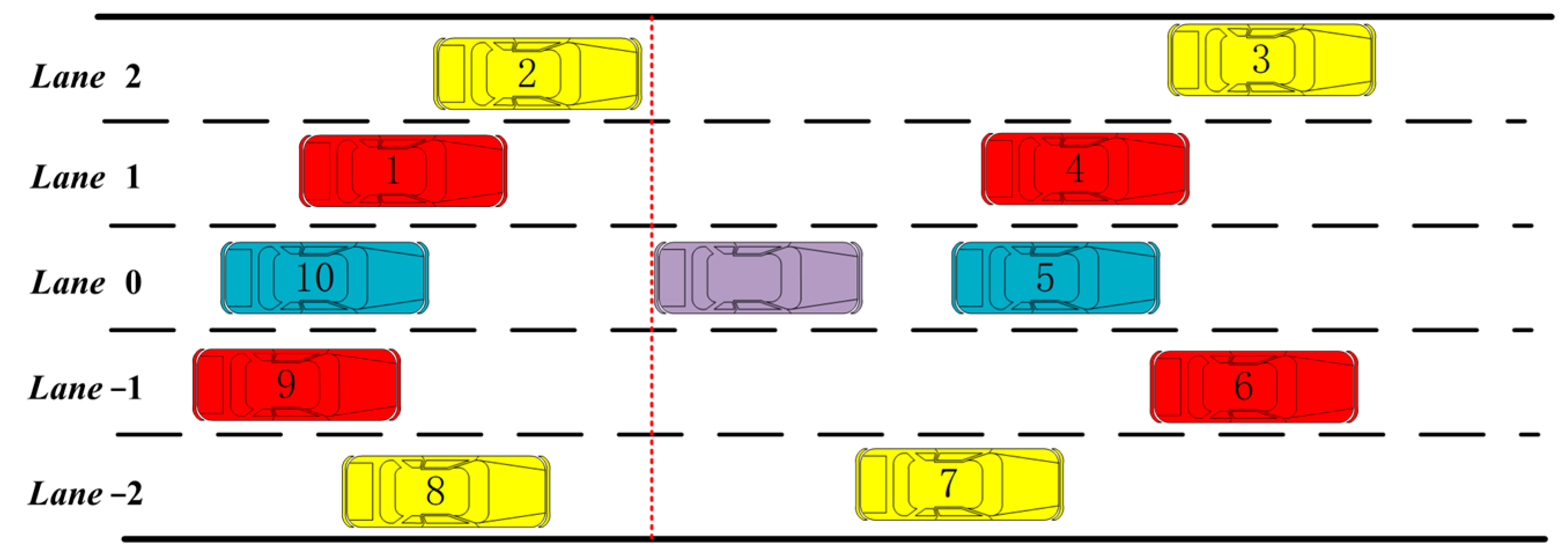
2.2.1. Classification of Surrounding Vehicles

When monitoring the relative motion state of the self-driving car and the surrounding vehicles in real time, the other vehicles on the road can be divided into vehicles in front and behind using the rear of the self-driving car as the dividing line and marking the lanes, as shown in Figure 2.
In Figure 2, i denotes the lane and takes values in the range: [0, 1, 2, −1, −2], which denotes the lane where the self-driving car is currently located, the adjacent lane on the left, the second adjacent lane on the left, the adjacent lane on the right, the second adjacent lane on the right, etc., respectively. In the case where the rear of the vehicle is the boundary, (i, fm) and (i, rm) denote the mth vehicle behind the vehicle and the mth vehicle in front of the vehicle in lane i, respectively. The range of lateral distances Δe between the self-driving vehicle and the surrounding vehicles can be calculated by Equation (4):
i = 0 | Δ e | d 1 d ov 2 + d v 2 1 d ov 2 + d v 2 Δ e 2 d 1 d ov 2 + d v 2 1 d ov 2 d v 2 Δ e 2 d 1 + d ov 2 + d v 2 2 d 1 + d ov 2 + d v 2 Δ e 3 d 1 d ov 2 + d v 2 2 d 1 d ov 2 d v 2 Δ e 3 d 1 + d ov 2 + d v 2
where dov, dv, and d1 denote the width of the other vehicle, the width of the self-driving vehicle, and the width of the lane, respectively.

2.2.2. Division of Surrounding Vehicle Behavior

When a vehicle travels on an expressway, the acceleration and heading angle changes are usually not very large. Therefore, it can be assumed that the vehicle’s acceleration and cross-swing angular velocity are constant within the predicted field of view [20]. Based on this assumption, the predicted vehicle velocity and yaw angle are shown in Equation (5):
v t = a 0 t + v 0 ψ t = γ 0 t + ψ 0
where a0 is the vehicle acceleration at the initial moment and r0 is the rate of change of the vehicle heading angle at the initial moment. v0 and ψ0 denote the predicted vehicle velocity and the heading angle at the initial moment, respectively.
According to the vehicle kinematic model, the vehicle velocity in the Cartesian coordinate system is shown in Equation (6):
v x t = v t cos ψ t v y t = v t sin ψ t
The parameters vxt and vyt are the vehicle’s velocity in longitudinal and transverse directions, respectively, at the prediction moment t.
At the initial moment, the longitudinal and transverse positions of the vehicle are x0 and y0, respectively, and the integration of the velocity v gives the vehicle’s trajectory at the future moment t, as shown in Equation (7):
x t = a 0 γ 0 2 cos ψ t + v t γ 0 sin ψ t a 0 γ 0 2 cos ψ 0 v 0 γ 0 sin ψ 0 + x 0 y t = a 0 γ 0 2 sin ψ t v t γ 0 cos ψ t a 0 γ 0 2 sin ψ 0 + v 0 γ 0 cos ψ 0 + y 0
L ( t ) = ( x t , y t )
The vehicle’s trajectory can be represented by Equation (8), which is obtained after the prediction of the vehicle kinematic model. The trajectory prediction is completed by determining the driving behavior of the vehicle in question to output the corresponding decision. The driving state of a vehicle is determined by its position on the current lane centerline. As shown in the figure below, we divide the lane into five zones and determine the vehicle’s driving behavior based on the predicted vehicle trajectory position. Therefore, the driving behavior of the surrounding relevant vehicles can be represented by the vehicle state identification function In(i,jn), as shown in Equation (9):
I n ( i , j n ) = 0 L a n e   k e e p i n g 1 L a n e   d e p a r t u r e 2 L a n e   c h a n g e   t o   t h e   l e f t 2 L a n e   c h a n g e   t o   t h e   r i g h t
where 0, 1, 2, and −2 indicate that the vehicle is currently in lane keeping, lane deviating, or lane changing to the left or right, respectively.

2.2.3. Division of Surrounding Vehicle Behavior and External Factors

When a vehicle travels on a multilane expressway, the driver can change lanes to the left or right. Therefore, the adjacent lanes need to be defined considering the safety state of the lanes to the left and right of the self-propelled vehicle and the driving state of the surrounding vehicles. A diagram of the driving behavior of adjacent lanes and vehicles is shown in Figure 3.
In order to fully consider the safety status of the left and right lanes of the self-driving car, we can summarize the traffic status on the left or right side of the self-driving car into five situations:
  • There needs to be more space in the adjacent lane for the self-driving car to change lanes;
  • There is sufficient space in the adjacent lane to make a lane change and no vehicles in the second to adjacent lane need to be considered for lateral movement;
  • There is sufficient space in the adjacent lane for a lane change and the vehicle in front of the vehicle in the second to adjacent lane needs to consider lateral movements;
  • There is sufficient space in the adjacent lane for a lane change and the vehicle behind the vehicle in the second to adjacent lane needs to be considered for lateral movement;
  • There is sufficient space in the adjacent lane for a lane change and the vehicles in front of and behind the vehicle in the second to adjacent lane need to be considered for lateral movement.
The safety posture of the target lane is classified according to the lateral movement of the vehicle and the adjacent lane to the left of the vehicle is considered. The safety posture is marked with a safety level of D. The lane-keeping, lane-deviating, and lane-changing states of the associated vehicle have an increasing effect on the adjacent lane. Specifically, the safety level can be divided into the following four cases:
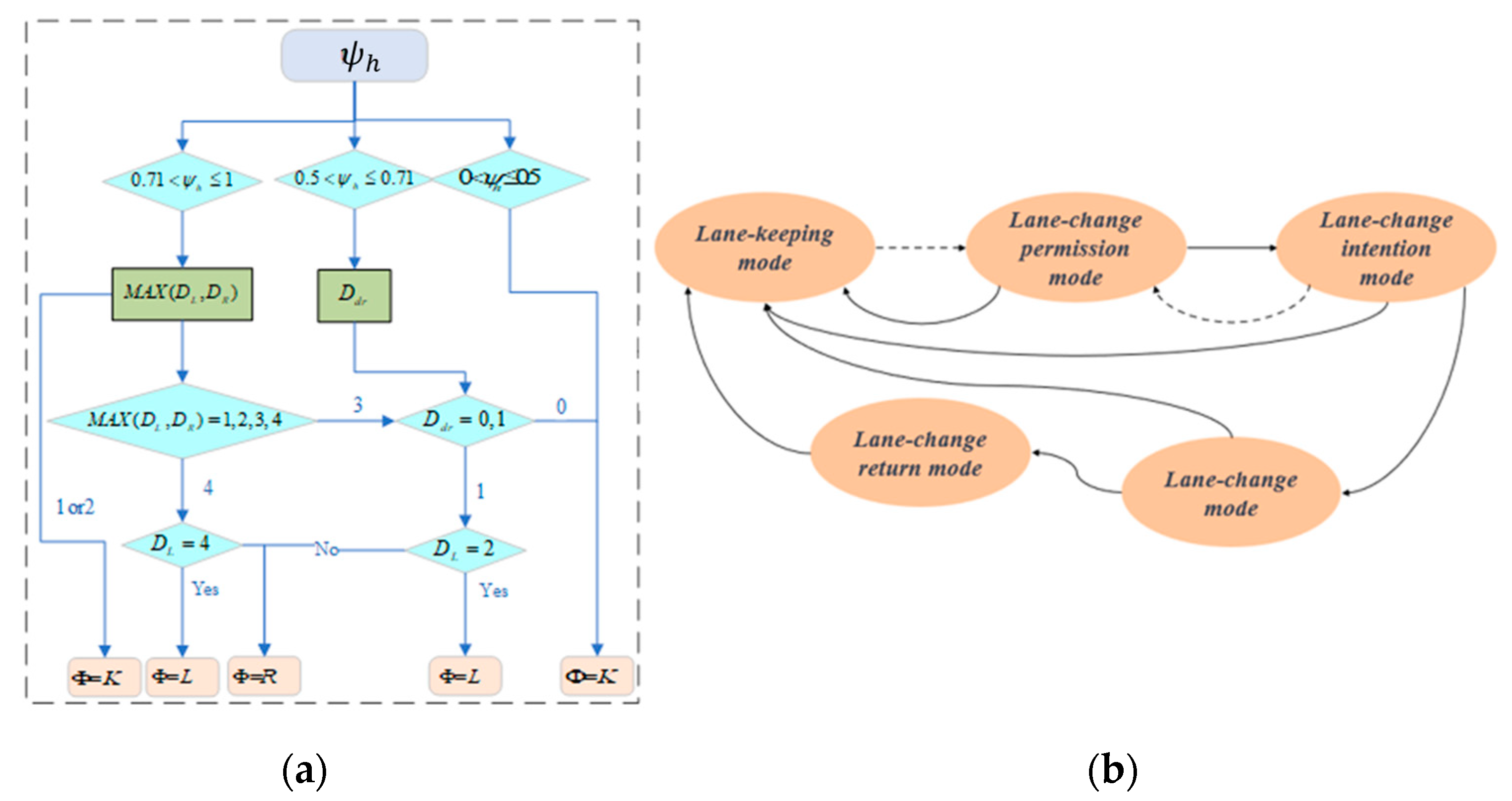
  • If there is no space for a lane change in the adjacent lane on the left, the safety level of the target lane is recorded as 1;
  • If there is space to change lanes in the adjacent lane on the left and an associated vehicle is changing lanes into the target lane, the safety level of the target lane is recorded as 2;
  • If there is space for a lane change in the adjacent lane on the left and the associated vehicle is in a lane departure, the safety level of the target lane is recorded as 3;
  • If there is space to change lanes in the adjacent lane on the left and there is no associated vehicle in a lane departure, the safety level of the target lane is recorded as 4;
When driving a self-propelled vehicle, it is necessary to consider the lateral movement of the surrounding vehicles as well as their longitudinal movement to avoid tailgating or being tailgated. When other vehicles appear in front of the self-driving vehicle, based on the fuzzy theory in the previous section, the lane change intention algorithm must be used to determine whether a lane change is required based on the actual situation. At the same time, the longitudinal movement state of the surrounding adjacent lanes needs to be further considered to ensure the safety of the target lane. In this paper, the optimized GIPPS safety model is used as a criterion for the safety state of the adjacent lane of the self-driving car. The vehicles nearest to the vehicle in front of the vehicle in the lane where the vehicle is located and the vehicles nearest to the vehicle in front and behind the vehicle in the adjacent lane are defined as the vehicles requiring consideration in the longitudinal state; the identification functions of these vehicles are defined as shown in Equation (10):
i , j n v r m v p = ± 2 , q = f , r 1 , f m
After combining the identification functions of the vehicles, the security posture level around the self-driving vehicle is shown in Equation (11):
D r e f = 1 D r e f = 4 I n 2 , f m 1 , 2 3 I n 2 , f m = 1 2 I n 2 , f m = 2 D r e f = 4 I n 2 , f m 1 , 2 I n 0 , r m 1 , 2 3 I n 2 , f m 2 I n 0 , f m 2 I n 2 , f m = 1 I n 0 , f m = 1 2 I n 2 , f m = 2 I n 0 , r m = 2 D r e f = 4 I n 2 , f m 1 , 2 I n 0 , q m 1 , 2 3 I n 1 , f m 2 I n 3 , q m 2 I n 1 , f m = 1 I n 3 , f m = 1 I n 3 , r m = 1 2 I n 1 , f m = 2 I n 3 , f m = 2 I n 3 , r m = 2
In addition, some of the external factors have an important influence on lane-changing behavior and vehicle operation. These factors should be considered in the modelling and lane-changing decisions. Different weather conditions, such as rain, snow, or fog, can have an impact on road visibility and vehicle performance. In these weather conditions, slippery road surfaces, reduced visibility, or reduced vehicle performance may lead to more difficult and dangerous lane-changing behavior. Therefore, when making lane-changing decisions, the model should consider the weather conditions and adjust the safety and appropriateness of lane-changing operations accordingly.
The road condition information includes factors such as traffic flow, road conditions, and road speed limits. Changes in traffic flow may affect the feasibility and safety of lane changing and more careful lane changing may be required during high traffic. In addition, road conditions such as road construction, road damage, or congestion need to be considered. The model should utilize sensors and communication technologies to obtain real-time road condition information and incorporate it into the consideration of lane-change decisions.
Construct a correction matrix Q shaped as Equation (12) describing the external disturbances.
Q = q rain q wind q fog q road
In Table 3, based on the approximate range of weather conditions, the penalty level for the correction factor is determined. Consider the effect of rain: when the precipitation is less than 0.1 mm per hour, it is considered to have a negligible effect on the intention to change lanes and q is recorded as 0; when the precipitation is in the range of 0.1~0.5 mm per hour, q is recorded as 1; when the precipitation is in the range of 0.5~4 mm per hour, q is recorded as 2; and when the precipitation is more than 4 mm per hour, q is recorded as 3. Consider the effect of wind: when the wind is in the range of 0~3 on the Beaufort scale, it is considered that the effect on the intention to change lanes is negligible and q is recorded as 0; when the wind is at 4~6 on the Beaufort scale, q is recorded as 1; when the wind is at 7~9 on the Beaufort scale, q is recorded as 2; when the wind is at 9~12 on the Beaufort scale, q is recorded as 3. Consider the effects of fog: when visibility is at 3.1~6.2 mile, it is considered that the effect on the intention to change lanes is negligible and q is recorded as 0; when the visibility is 0.6~3.1 mile, q is recorded as 1; when the visibility is at 0.1~0.6 mile, q is recorded as 2; when the visibility is less than 0.1 mile, q is recorded as 3. Consider the effect of the road surface conditions: when the road surface is in a dry condition, q is recorded as 0; when the road surface is in a damp condition, q is recorded as 3. When the road surface is in damp state, q is written as 1; when the road surface is in a stagnant water state, q is written as 2; when the road surface has snow and ice cover or is in a muddy state, q is written as 3.
When each adjustment factor in the correction matrix of the self-driving vehicle is 0, i.e., the influence of each external factor is small, ||Q|| = 0 and the intention to change lanes is not corrected. When the self-driving vehicle is in a situation where there is a strong external interference, in order to ensure safety, the original intention to change lanes needs to be corrected. The corrected lane-change intention is shown in Equation (13):
D L = D r e f | | Q | | D R = D r e f | | Q | |
In the equation, DL represents the safety level rating of the adjacent lane on the left side of the ego vehicle. Similarly, DR denotes the rating of the adjacent lane on the right side. A higher value of the safety level parameter DL or DR indicates a safer surrounding environment for the ego vehicle.
The upper two subsections devise a lane-change willingness based on fuzzy theory and classify the safety levels of the adjacent lanes of the self-driving car, solving the problem of determining when to change lanes, whether it is safe to do so around the self-driving car, and whether there are conditions for changing lanes. These two parts are combined to form a complete driving logic, as shown in Figure 4a. Based on this driving logic, a decision based on a finite state machine is designed, as shown in Figure 4b. In the figure, the values K, L, and R of φ indicate lane keeping, lane changing to the left, and lane changing to the right, respectively. The specific flow of the decision is as follows: when the willingness to change lane ψh is derived, a judgement in made to determine whether the vehicle needs to change lanes. A DL/DR value of 4 means that the left and right adjacent lanes are safe for lane changing, whereas a DL/DR value of 3 means that a lane change is required based on the driver’s style. No lane change is required if the driver style parameter Ddr value is 0. If the value of Ddr is 1, the next step is to determine if the associated vehicle has not changed lanes, then there is room for the self-driving vehicle to change lanes. Otherwise, no lane change is allowed. The fuzzy control table can set the driver style in the fuzzy lane-change intention controller. To ensure the safety of the self-driving vehicle throughout the lane change process, the vehicle’s safety posture monitoring of the target lane is permanently active.
In Figure 4b, the circles indicate the states in the state machine and the arrows indicate the direction of the state transfer. The lane-keeping state of the vehicle driving in the current lane is the default state, and the state transfer will be triggered when the condition is satisfied.

3. Intelligent Vehicle Trajectory Planning and Control

3.1. Intelligent Lane-Change Trajectory Planning

In practical scenarios, vehicles must travel to their destinations based on the global paths planned by high-precision map navigation systems to obtain rough reference trajectories and driving directions [21,22]. However, the vehicle always encounters unknown environmental uncertainties during the driving process, thus making the global path challenging for ensuring the safe driving of the vehicle and unable to meet the driving requirements of the vehicle. In this paper, the global path is assumed to be known and the global path and the lane change operation are considered together. The intelligent vehicle plans its trajectory after the decision layer issues the lane change command.
In the lane-change scenario of the highway shown in Figure 5, the AV represents the autonomous vehicle in the current lane and the vehicle (DA) is driving in front of the autonomous vehicle. The target lane for the lane change (the left lane of the current lane) has two vehicles in it, i.e., the vehicle in front (FL) and the vehicle behind (RR). The vehicle behind the current lane (DS) is not considered as it is influenced by the autos (AV).
This paper uses a quintuple polynomial model for lane-change trajectory planning, and a trajectory planner based on a quadratic planning approach is designed to select the optimal candidate trajectory for different lane-change times while ensuring safety and comfort. During the lane change, the self-driving vehicle must transition smoothly to the target lane. The quintic polynomial has the advantages of high-order successive derivatives and computational simplicity and is, therefore, a well-established solution for planning lane-change trajectories. In this paper, both longitudinal and lateral trajectories are described using a fifth-order polynomial, as shown in Equation (14):
x ( t ) = a 0 + a 1 t + a 2 t 2 + a 3 t 3 + a 4 t 4 + a 5 t 5 y ( t ) = b 0 + b 1 t + b 2 t 2 + b 3 t 3 + b 4 t 4 + b 5 t 5 S 0 = X 0 , V x , 0 , a x , 0 ; Y 0 , V y , 0 , a y , 0 S f = X 0 , V x , f , a x , f ; Y f , V y , f , a y , 0
where Xf is vehicle longitudinal position, Vx,f is velocity, and ax is acceleration; the result can be obtained by solving the 12 linearly independent equations.
Driving safety must be considered when designing the QP solver to select the optimal collision-free trajectory. The minimum safe distance constraint must be satisfied to ensure the vehicle’s safety. The minimum longitudinal safety distance is the minimum longitudinal distance that needs to be maintained to avoid a collision when the self-driving vehicle is usually driving and there are other vehicles in the current lane. Therefore, the condition that no collision occurs between the self-driving vehicle AV and the preceding vehicle DA is shown in Equation (15):
t 0 , t C , X D A ( t ) 0.5 L D A > X A V ( t ) + 0.5 L A V + W A V × sin ( ψ )
where tC is the moment when the vehicle leaves the current lane; xAV, LAV, and WAV denote the longitudinal position, length, and width of the self-driving vehicle, respectively; XDA and LDA denote the longitudinal position and length of the vehicle in front, respectively; and ψ is the heading angle of the self-driving vehicle, take LDA = LAV.
Let:
L l 1 = 0.5 L D A + 0.5 L A V + W A V × sin ( ψ )
Then:
X A V ( t ) < X D A ( t ) L l 1 t [ 0 , t c ]
S l a = X D A ( t ) X A V ( t ) L l 1 > 0 t [ 0 , t c ]
S l a ( 0 ) + 0 t 0 λ ( a D A ( τ ) a A V ( τ ) ) d τ d λ + ( v x , D A ( 0 ) v x , A V ( 0 ) ) × t > 0 t [ 0 , t c ]
After analysis, it can be seen that only the minimum value of equation for the two vehicles is not to collide. Instead of the minimum longitudinal distance at the start of the self-driving vehicle lane change, Gipps’ [23] safety distance model is quoted, which is shown in Equation (16):
G D A ( t ) = V ( t ) x , A V × T s + V ( t ) x , A V 2 2 b A V , max V ( t ) x , D A 2 2 b D A , max t [ 0 , t c ]
where Vx,AV and Vx,DA denote the longitudinal velocity of the self-driving vehicle AV and the preceding vehicle DA, respectively; bAV,max and bDA,max are the maximum acceleration values for AV and DA, respectively; and Ts is the reaction time.
Rewriting the collision conditions is shown in Equation (17):
X D A ( t ) 1 2 L D A > X A V ( t ) + 1 2 L A V + G D A ( t ) t [ 0 , t c ]
Similarly, the collision conditions between the self-driving car AV and the adjacent lane front vehicle FL and rear vehicle RR can be obtained as in Equations (18) and (19):
X F L ( t ) 1 2 L F L > X A V ( t ) + 1 2 L A V + G F L ( t ) t [ t c , t f ] G F L ( t ) = V ( t ) x , A V × T s + V ( t ) x , A V 2 2 b A V , max V ( t ) x , F L 2 2 b F L , max t [ t c , t f ]
X R R ( t ) 1 2 L R R > X A V ( t ) + 1 2 L A V + G R R ( t ) t [ t c , t f ] G R R ( t ) = V ( t ) x , A V × T s + V ( t ) x , A V 2 2 b A V , max V ( t ) x , R R 2 2 b R R , max t [ t c , t f ]
Firstly, the travel time during the AV lane change is processed using equal interval sampling. Then, a trajectory planner based on the quadratic planning method is designed and safety- and comfort-related constraints are added. Finally, the optimal lane-change trajectory is selected by combining the driving efficiency. If the initial state and time of the AV lane change are a priori, the lateral trajectory can also be determined based on a quintic polynomial model of the lane-change trajectory. Therefore, only three end states of the AV need to be optimized, namely the longitudinal position Xf, the velocity Vx,f, and the acceleration ax.

3.1.1. Equally Spaced Sampling

During a lane change in an autonomous vehicle, the travel time is an essential indicator of safety, ride comfort, and driving efficiency. If the lane-change time is too short, the lateral acceleration increases, which leads to a decrease in vehicle smoothness. If the lane change time is too long, the danger of the journey increases and the efficiency of the journey decreases. Therefore, this paper designs the shortest lane change time, Tmin, and the longest lane change time, Tmax, and then optimizes the trajectory according to the different lane change times. The sampling time during the lane change is shown in Equation (20):
Δ T = T max T min / N t k f = k Δ T + T min , ( k = 0 , 1 , , N )
where ΔT is the sampling interval and N is the number of samples.

3.1.2. Boundary Conditions

The lateral position, velocity, and acceleration of the autonomous vehicle should be kept within the range shown in Equation (21):
W L 2 + W H 2 Y ( t ) 3 W L 2 W H 2 0 V x ( t ) V x , max a x , min a x ( t ) a x , max a y , min a y ( t ) a y , max

3.1.3. Cost Function and Its Optimal Solution

In an actual lane-change process, the autonomous vehicle usually completes the lane-change process as soon as possible while ensuring the comfort of the passengers. Therefore, both factors (efficiency and comfort) should be considered when finding the optimal lane-change trajectory. However, efficiency and comfort are two conflicting factors, so the optimal lane change trajectory needs to be able to balance these two factors. In this paper, a cost function is constructed to describe the effect of comfort and efficiency on the optimal lane-change trajectory of an autonomous vehicle, and safety and smoothness comfort factors are taken into account to solve for the optimal trajectory for different lane-change times. This paper uses the additive acceleration (jerk) evaluation metric to evaluate smoothness. The comfort cost function is shown in Equation (22):
J C X f , V x , f , a f = w x 0 t f j x ( t ) 2 + w y 0 t f j y ( t ) 2
where jx and jy denote the longitudinal and lateral accelerations of the self-driving car, respectively, and wx and wy are the weights.
Thus, the trajectory-planning problem using different numbers of samples can be transformed into an optimization problem, as shown in Equation (23):
min J X f , V x , f , a x , f = J C
W L 2 + W H 2 Y ( t ) 3 W L 2 W H 2 , 0 V x ( t ) V x , max a x , min a x ( t ) a x , max , a y , min a y ( t ) a y , max t 0 , t C , X P C ( t ) 1 2 L P C > X H ( t ) + 1 2 L H + G P C t t C , t f , X T P ( t ) 1 2 L T P > X H ( t ) + 1 2 L H + G T P t t C , t f , X H ( t ) 1 2 L H > X T F ( t ) + 1 2 L T F + G T F
Using a quadratic programming (QP) solver, the optimal longitudinal position, velocity, and acceleration of the self-driving vehicle at the end of the lane change can be solved by setting the planning time tk to determine the trajectory of the lane change.

3.2. Stability-Based Trajectory Tracking Control

The primary purpose of trajectory tracking control is to output the appropriate control quantity to make the intelligent vehicle travel according to the planned trajectory and improve the tracking accuracy while ensuring vehicle stability. In order to solve this problem, this paper designs the vehicle transverse pendulum stability envelope based on the three-degree-of-freedom vehicle dynamics model. Firstly, the phase planes of the angular velocity of the transverse pendulum and the unnatural angle of mass are established, the variation law of the equilibrium point and the saddle point in the phase diagram when the front wheels are turned is analyzed, and the vehicle stability boundary is designed in combination with the maximum lateral deflection angle of the front and rear wheels of the vehicle in order to improve the tracking accuracy by playing with the dynamic limit of the vehicle. At the same time, considering that the vehicle may roll over when performing the extreme motion, the anti-rollover constraint is established using the zero-moment point analysis method.

3.2.1. Vehicle Dynamics Model

This paper uses the three-degree-of-freedom monorail model shown in Figure 6 as the vehicle dynamics model. The model considers the dynamical coupling between the vehicle’s lateral velocity, longitudinal velocity, and rollover and describes the vehicle rollover dynamics using the properties of suspension damping and stiffness. Based on Newton’s laws, a system of equations can be obtained, as shown in Equation (24):
v ˙ y = F y r + F y f / m v x γ γ ˙ = F y f l f F y r l r / I z ϕ ¨ = m s h v ˙ y + v x γ + m s g h ϕ K ϕ D ϕ ˙ / I x e ˙ y = v x e φ + v y e ˙ φ = γ κ v x
where vx and vy are denoted as the longitudinal and lateral velocities of the vehicle body’s center, m is the vehicle’s center of gravity mass, ms is the mass on the springs, γ is the vehicle transverse angular velocity, φ is the vehicle heading angle, β is the vehicle center of mass lateral deflection angle, f is the front wheel turning angle, Ix and Iz denote the body rotational inertia around the x and z axes, respectively, Lf and Lr are the distances from the vehicle’s center of gravity to the front and rear axles, respectively, Tr and h are the wheelbase and center-of-mass height, Fyf and Fyr are the lateral forces of the front and rear wheels, and ϕ is the lateral camber angle of the vehicle. It is the curvature of the road. Kϕ and Dϕ are the vehicle lateral stiffness coefficient and damping coefficient, respectively, and ey and eφ are the lateral deviations and heading angle deviation of the vehicle from the reference path, respectively.
In path following control, nonlinear tire characteristics are considered to exploit the vehicle’s extreme performance, and the lateral tire forces are modeled using the magic formula tire model. The model is shown in Equation (25):
F y = μ D y C y arctan ( B y α + E y B y α arctan B y α
where Cy is the shape factor, By is the stiffness factor, Dy is the peak value, and Ey is the curvature value; the above parameters are related to the magnitude of the tire’s droop force. α is the tire slip angle. μ is the road adhesion force. To obtain the real-time nature of the calculations, the magic tire model was linearized; the results are shown in Equation (26):
F y = C ¯ α f , r α f , r

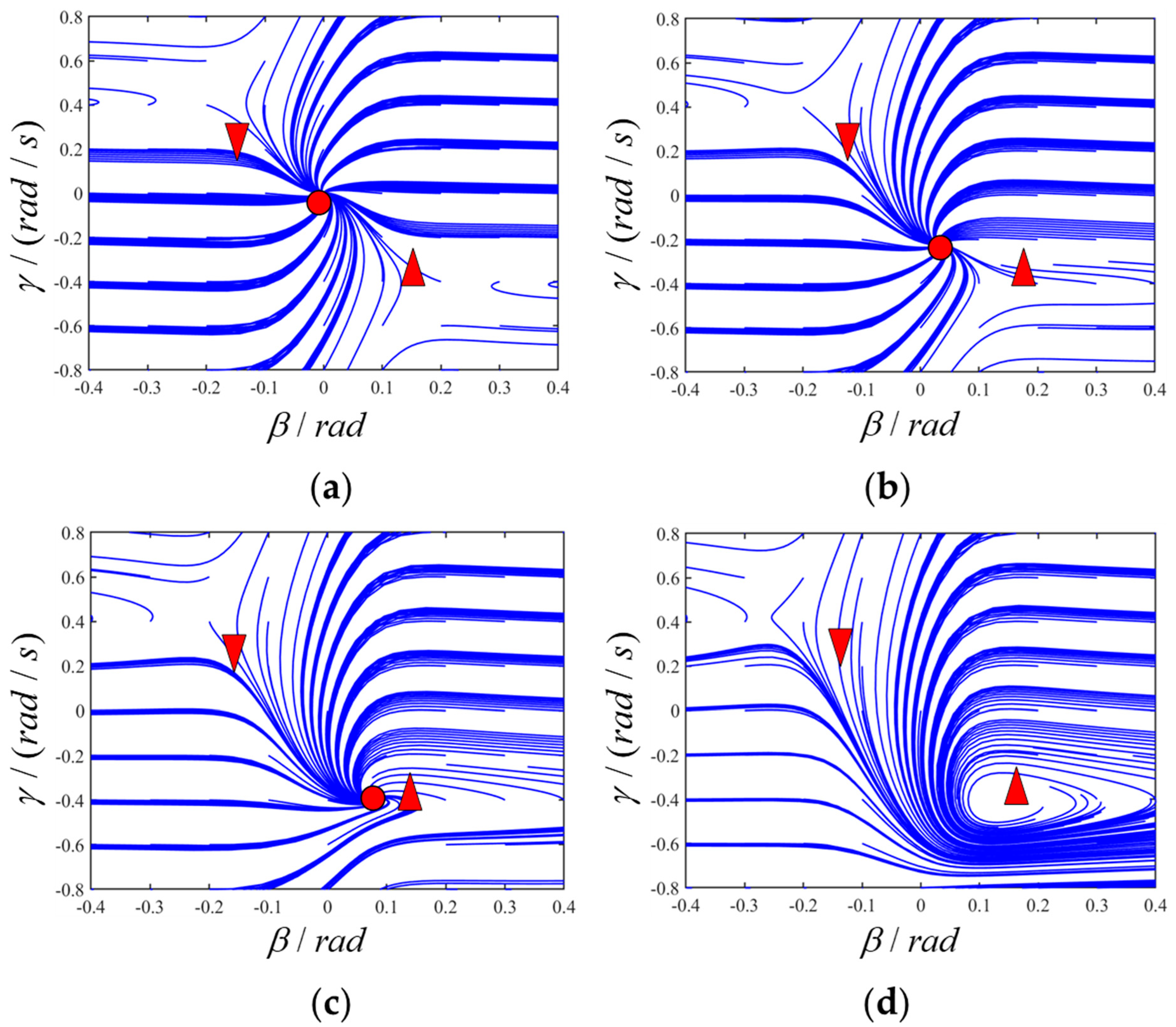
3.2.2. Vehicle Stability Constraints

In order to improve the lateral stability of the vehicle, this paper analyses the variation law of the front wheel turning angle and phase plane based on a three-degrees-of-freedom vehicle dynamics model, establishes a stability envelope curve to determine the stability domain, and derives reasonable stability constraints. For the lateral stability of the vehicle, when designing the anti-rollover constraint, the moment normalization is first carried out and then the various positions of the zero-moment points are analyzed; the zero-moment point when a rollover is about to occur is taken as the condition to prevent the vehicle from rolling over.
  • Vehicle Lateral Stability Constraint
When the vehicle is steering, if the steering angle increases to a certain angle, the lateral force of the tire will enter the nonlinear saturation region and the vehicle will quickly become unstable. When the lateral force of the front or rear wheel is saturated, the vehicle will quickly lose its steering ability and be unable to track the desired trajectory or produce destabilizing maneuvers such as tailing. Therefore, two parameters, the center-of-mass lateral deflection angle and the angular velocity of the transverse sway, are used to characterize the vehicle’s stability when the center-of-mass lateral deflection angle is slight, thereby improving the accuracy of the vehicle tracking trajectory.
A phase-plane diagram is used to graphically demonstrate the system’s dynamics, allowing the location of the equilibrium point and the stability region of the system to be identified graphically. For the vehicle dynamics model, the differential equation between γ and β is established, as shown in Equation (27):
γ ˙ = 2 L f F y f cos δ f 2 L r F y r I z β ˙ = 2 F y f cos δ f + 2 F y r m v x φ ˙
when vx is 98 km/h and μ is 0.85, the phase-plane diagrams for front wheel steering angles f of 0 rad, −0.12 rad, −0.20 rad, and −0.31 rad are shown in Figure 7. In the diagrams, the balance points are indicated by red dots and the saddle points by red triangles.
Figure 7 shows the phase plan under different front wheel angles, which are 0 rad, 0.12 rad, 0.20 rad and 0.31 rad, respectively. Figure 7a–d shows that as the front wheel angle increases, the equilibrium point of the system gradually shifts from the origin to the lower right and the stable state of the system gradually changes. As the absolute value of the front wheel angle continues to increase, the equilibrium point moves towards the saddle point in the lower right. The equilibrium and saddle points meet when the front wheel angle is at its maximum value. If the front wheel angle increases, the equilibrium point will disappear and the vehicle will enter an unstable state.
For the vehicle to reach the maximum instantaneous limit performance that it can perform, the vehicle dynamics stability limit and the state of imminent destabilization should be kept in line. The analysis of the phase-plane diagram shows that the vehicle steady-state zone limit is related to the position of the saddle point. In general, the lateral stability limit of the vehicle can be expressed in terms of the lateral deflection angle corresponding to the maximum lateral deflection angle of the rear wheels. Therefore, the maximum value of the center-of-mass lateral deflection angle can be calculated using the maximum lateral deflection angle of the rear wheels. The lateral deflection angle increases when the front wheel steering angle increases. Suppose the front wheel lateral deflection angle reaches its maximum value. In that case, the vehicle will tend towards extreme understeer, which may lead to instability. When the front wheel lateral deflection angle reaches its limit should also be considered. Therefore, the vehicle stability criterion should be designed by combining the corresponding maximum/minimum side deflection angles of the front/rear wheels and the saddle point position.
The maximum/minimum side deflection angles I and −I, determined from the rear wheels, are shown in Equation (28):
I = L r γ v x tan α s , r I = L r γ v x + tan α s , r
where αs,r is the maximum lateral deflection angle of the front wheels.
The straight-line H and −H, determined from the saddle point, are shown in Equation (29):
H = μ g v x H = μ g v x
Figure 8 shows stability boundary under different front wheel angles, which are 0 rad, 0.12 rad, 0.20 rad and 0.31 rad, respectively, at 98 km/h. It can be observed from Figure 8a,b that the position of the vehicle equilibrium point and the stability boundary are related to the corresponding maximum/minimum side deflection angles of the front/rear wheels. As the front wheel turning angle increases, the equilibrium point gradually converges from (0, 0) to the saddle point position, whereas J and −J change accordingly, forming the stability boundary. When the front wheel turning angle reaches −0.20 rad, lines H and J intersect near the saddle point in Figure 8c, indicating that the vehicle is in a critical state. If the steering angle continues to increase, the saddle point will disappear and the J and −J envelopes defined by the front wheels and H and −H, I, and −I will not be able to form a closed envelope area, which means the vehicle will tend to be unstable, as shown in Figure 8d.
Assuming that the longitudinal speed vx of the vehicle remains constant, a stability boundary for the lateral stability of the vehicle can be derived by considering the maximum/minimum transverse sway speed near the saddle point, the maximum/minimum range of lateral deflection angles determined for the front and rear wheels, and the maximum/minimum stable steering angle of the front wheels at the current vehicle speed. This stability domain can be expressed by the inequality shown in Equation (30):
λ 1 λ 0 γ β λ 1 λ 3 γ λ 2 β λ 3
Combined with the system-state space equations, the lateral stability criterion based on this envelope at each moment in time is shown in Equation (31):
I s ( k ) V s ( k ) η ( k ) I s ( k )
where
V s ( k ) = 1 / v x λ 0 0 0 0 0 λ 2 / v x 1 0 0 0 0 I s ( k ) = λ 1 λ 3 λ 0 = L r v x λ 1 = tan ( α s , r ) λ 2 = v x L r λ 3 = v x L r tan ( α s , r )
After calculation, the controller constraint formed by this closed envelope is obtained to ensure the lateral stability of the vehicle.
2.
Vehicle Lateral Stability Constraint
Vehicle lateral stability is essential for travel, especially under extreme high-speed conditions and large curvatures. In these cases, the zero-moment point is a crucial concept, representing the point on the ground where the sum of the roll moments due to gravity and inertial forces acting on the vehicle is zero [3].
A predetermined zero-moment point predicts the risk of wheel lift if the front wheel angle is inappropriate. Therefore, the zero-moment point can be used as an anti-rollover constraint for the model predictive controller to reduce the risk of rollover by normalizing the zero-moment point to the front wheel steering angle. The normalization of the lateral offset yZMP of the zero-moment point concerning the wheelbase is shown in Equation (32):
y ¯ Z M P = 2 T r [ h ϕ + h g ( v ˙ y + γ v x ) I x ϕ ¨ m g ]
Combined with the system-state space equations, yZMP can be expressed in the form shown in Equation (33):
y ¯ ( k ) Z M P = N 1 X ˙ ( k ) + N ˙ 2 X ( k )
where
N 1 = 2 h / g T r 0 2 I x / m g T r 0 0 0
N 2 = 0 2 h v x g T r 0 2 h T r 0 0
The stability constraint on vehicle roll can be expressed in the form shown in Equation (34):
y ¯ l y ¯ ( k ) Z M P y ¯ l
From experience:
y ¯ l [ 0.60 , 0.95 ]

3.3. Model Predictive Controller Design

This section proposes a path-tracking controller for driverless vehicles based on a model predictive control algorithm. Vehicles applying this controller can ensure the accuracy of path tracking, yaw stability, and anti-roll capability under various operating conditions. The control framework has been given as Figure 9.
In order to obtain a linear time-varying model, the state space equations are discretized according to the sampling time in the form shown in Equation (35):
ξ ( k + 1 ) = A s ξ ( k ) + B s 1 u 1 ( k ) + B s 2 u 2 ( k ) y ( k ) = C x ( k )
where
A s = I N + A t s B s 1 = B 1 t s B s 2 = B 2 t s
The controller represents the path tracking problem as an optimization problem within each execution cycle to minimize the error between the vehicle’s lateral position and the desired road trajectory. To this end, an optimization function, as shown in Equation (36), is developed in conjunction with the discrete model of the vehicle in equation:
min k = 1 N p y ( k , t ) y r e f ( k , t ) Q 2 + u 1 ( k , t ) u 1 ( k 1 , t ) R 2
s.t.
ξ ( k + 1 ) = A s ξ ( k )   +   B s 1 u 1 ( k )   +   B s 2 u 2 ( k ) k I s ( k ) V s ( k ) η ( k ) I s ( k ) k = 1 , , N y ¯ l y ¯ ( k ) Z M P y ¯ l k = 1 , , N Δ M M ( k ) M ( k 1 ) Δ M k Δ δ f δ f ( k ) δ f ( k 1 ) Δ δ f k
where Q, R is the weight matrix used to represent the weights of the terms in the optimization problem. The optimization function’s first term represents the vehicle’s deviation relative to the reference path, and the second term ensures smoothness of control. The constraints include vehicle dynamics, lateral stability, and lateral sway constraints. In addition, other lateral moments M and front wheel turning angles are also constrained to ensure controller performance.
In the optimization function, the sequence of states in the prediction range and the optimal control sequence are expressed in the form shown in Equation (37):
ξ k = ξ k + 1   k , , ξ k + N   k T u k = u k   k , , u k + N 1   k T
Only the first term of the control sequence, uk, is taken as the control input to the vehicle to complete the control of the vehicle.

4. Simulation Experiments

In this section, the joint simulation of intelligent vehicles under high-speed multilane conditions is carried out using PreScan2019.1, Carsim 8.5, matlab 2020a.to build a common simulation platform to verify the vehicle’s decision layer, planning layer, and controller. Road scenarios, including other traffic participants and road models, were built in PreScan and the corresponding algorithms were designed in Matlab/Simulink. The co-simulation framework has been given as Figure 10.

4.1. Follow the Driving Conditions

At the initial moment, the car in front is driving slowly and the adjacent lanes on the left and right cannot change lanes; the self-driving care follows the car with the longitudinal distance and speed of the car in front as a reference. The local traffic state is shown in Figure 11a; the initial longitudinal distance between the self-driving car and car 1 is 100 m, and the initial longitudinal distance between the self-driving car and cars 2 and 3 is 20 m and 25 m, respectively. The initial speed of the self-driving car is 33 m/s, the driving speed of car 1 is 20 m/s, and cars 2 and 3 travel at constant speeds of 22 m/s and 20 m/s, respectively.
The relative longitudinal distance between the self-propelled vehicle and vehicle 1 in front of it is 100 m when it travels in the current lane, which is less than the safe distance Dsafe and is therefore a dangerous traveling distance. At the same time, the longitudinal distance between the vehicle and vehicle 2 and vehicle 3 is so close that it is impossible to change lanes. In this case, the autocar can only brake and slow down, using the speed and relative longitudinal distance of vehicle 1 as a reference for following the vehicle. At 7 s, the speed of the self-driving car is equal to the speed of vehicle 1, at which point the distance between the two vehicles remains at around 71 m, as shown in Figure 11b. Until the end of 10 s, there is no rear-end collision between the self-driving vehicle and vehicle 1 and the minimum safe distance model LfDsafe is satisfied, as shown in Figure 11c.
According to Figure 12a, when the longitudinal distance is less than the minimum safe distance, the decision process can cause the car to brake immediately, quickly decelerating and avoiding a rear-end accident. Meanwhile, according to Figure 12b, the vehicle can quickly plan the appropriate speed to decelerate from 33 m/s to the same 20 m/s as vehicle 1 with a deceleration rate of −3 m/s2, which does not affect the smoothness of the vehicle too much and also satisfies the minimum safe distance model. In addition, the speed tracking controller can track the reference speed in time. Figure 12c reflects the safety level of the adjacent lane of the self-propelled vehicle, which is always 1, as there is no space for lane changing on either side.

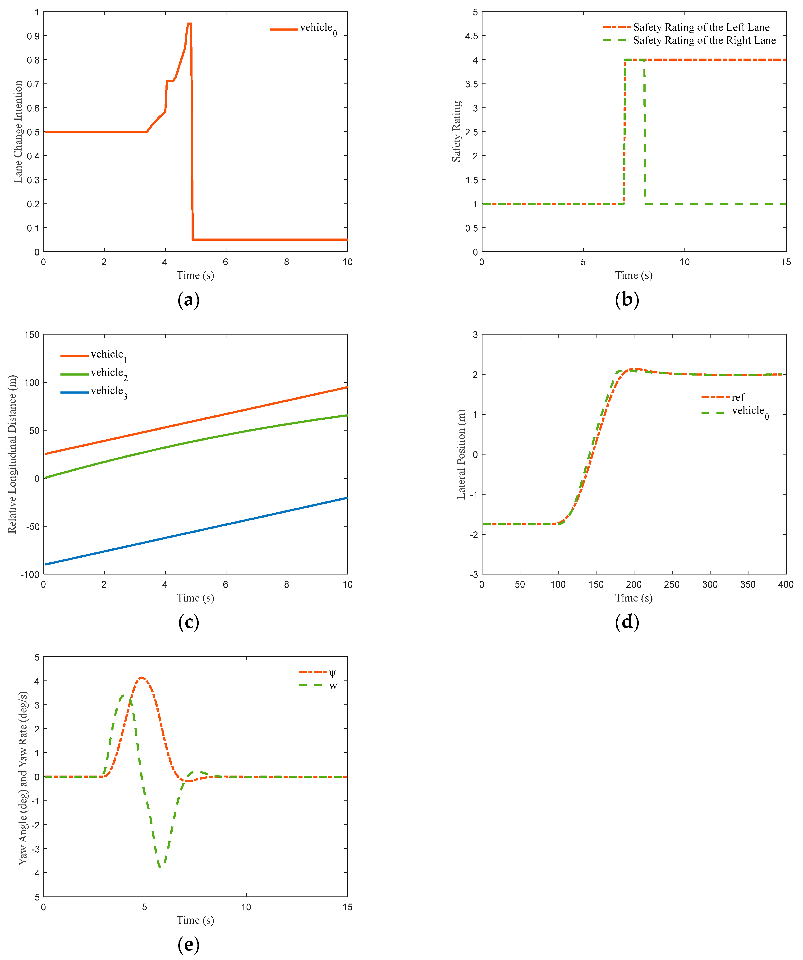
4.2. Constant Speed Lane-Change Conditions

This scenario simulates a vehicle making a high-speed lane change with room to change lanes on the left. The local traffic state at the initial moment is shown in Figure 13a, where the initial longitudinal relative distance between the self-driving car and car 1 is 90 m and the initial longitudinal relative distances with cars 2 and 3 are 5 m and 25 m, respectively. The self-driving car travels at a constant speed of 27 m/s, whereas car 1, car 2, and car 3 travel along their current lanes at 20 m/s, 18 m/s, and 20 m/s, respectively.
According to Figure 13b, when the car is traveling for 4 s, the longitudinal relative distance Lf between the car and the car in front of it is equal to the minimum safe distance Dsafe. As there is no space to change lanes on the right side of the car, the car can only change lanes to the left. After 7.5 s, the car has completed the lane change and enters lane 2. According to Figure 13c, the relative longitudinal distance between the car and the car before and after the lane change is greater than the minimum safe distance Dsafe, indicating that the planned lane-change trajectory meets the obstacle avoidance requirements. According to Figure 13d, the main car completed the entire lane change process.
The safety state of the self-driving vehicle is shown in Figure 14b. At the initial moment, the safety level of the autonomous vehicle’s left and right adjacent lanes is 1 until 7.5 s, when the autonomous vehicle completes the lane change from lane 3 to lane 2. When the car has completed the lane change, lane 1 becomes the left lane of the car. At this point, both the three cars in that lane and the two cars in lane 1 are at a safe distance from the car and the safety level to the left of the car becomes 4. Lane 3 becomes the right lane of the car. For nearly 1 s after the lane change is completed, the longitudinal safety distance between the self-driving car and car 1 satisfies the minimum safety distance. However, 8 s later, the distance between the self-driving car and car 1 decreases and the safety level on the right side changes to 1.
As can be seen from Figure 14c, the planned lane-change trajectory is smooth and reasonable and meets the lane-change requirements. As shown in Figure 14d, the maximum lateral displacement error for the controller designed in this paper is 0.25 m when performing a high-speed lane change, which meets the requirements of vehicle accuracy. In addition, as shown in Figure 14e, the transverse pendulum angle and angular velocity are within a reasonable range.

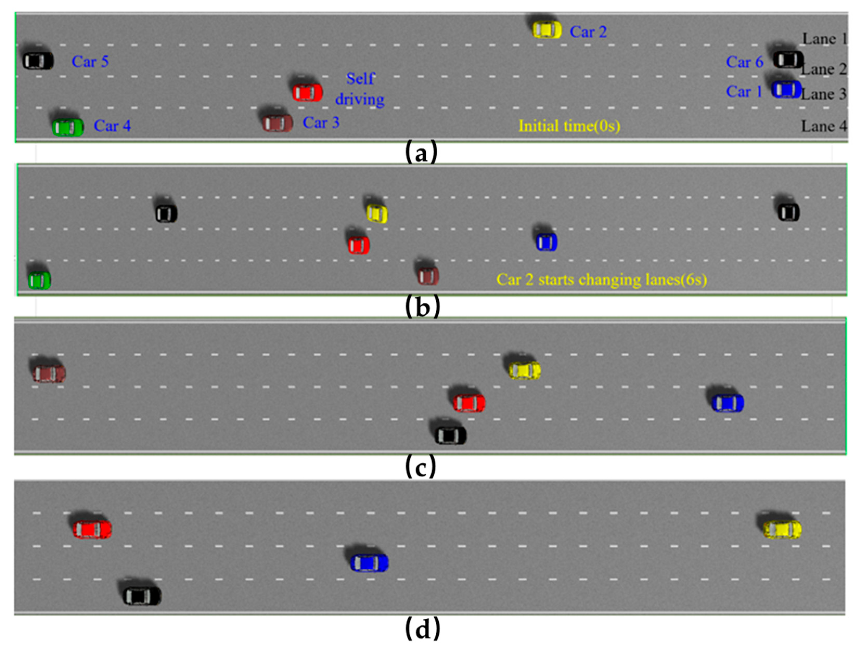
4.3. Simultaneous Lane-Change Conditions

This scenario simulates the situation of a self-driving car changing lanes to overtake and other vehicles suddenly merging into the target lane. In this scenario, a third vehicle travels along lane 1 for 3 s before suddenly changing lanes into lane 2 at 33 m/s, as shown in Figure 15. The local traffic state at the initial moment is shown in Figure 15a. In the initial state, the longitudinal distance between the self-driving car and car 1 is 60 m and the longitudinal distances between the self-driving car and cars 2 and 3 are 1 m and 26 m, respectively. The self-driving car travels at a constant speed of 25 m/s, whereas cars 1, 2, and 3 travel along the current lane at 20 m/s and 18 m/s.
According to Figure 15b, car 3 enters the lane change at 3 seconds but has yet to cross the lane line fully. Although the relative longitudinal distance Lr between the car and car 2 and the longitudinal relative distance Lf of car 1 meet the minimum safety distance requirement of Lr and LfDsafe, the safety level of the surrounding adjacent lane is 2; therefore, the safety conditions for lane change are not met. Therefore, the self-driving car decides to slow down and maintain the current lane until it is equal to the speed of the one car ahead. When the third car fully enters the second lane, the safety level of the adjacent lane of the self-driving car will all change to 1. By the 7th second, the longitudinal relative distance Lf between the self-driving car and the third car reaches a safe distance and the safety level on the left side of the self-driving car is raised to 4. At this point, the self-driving car changes lanes to overtake the first car and enters the second lane; the safety level of the adjacent lane of the self-driving car is shown in Figure 16d. The intermediate process of lane change is shown in Figure 15c. According to Figure 15d, the main car completed the entire lane change process.
As can be seen from Figure 16a, the self-driving car maintains a reasonable longitudinal distance from the surrounding vehicles during the journey, ensuring safe driving. As shown in Figure 16b, when three vehicles suddenly change lanes, the self-driving car can delay the lane change according to its state change, ensuring safe driving. In addition, according to the speed change curves of the self-driving car and the one car ahead in Figure 16c, we can see that when there is no lane-change condition, the self-driving car can cruise at the speed of the previous car to maintain a safe distance in front and behind it until it finishes the lane change and then accelerates to reach the preset desired speed. The driving decisions designed in this paper consider whether to change lanes but also the safety of the adjacent lanes. As shown in Figure 16d, if the self-driving car makes a lane change at the 3.3 s mark, it will collide with car 3. Therefore, the self-driving car decides to slow and stay in the same lane until it is equal to the speed of car 1 ahead, ensuring driving safety.

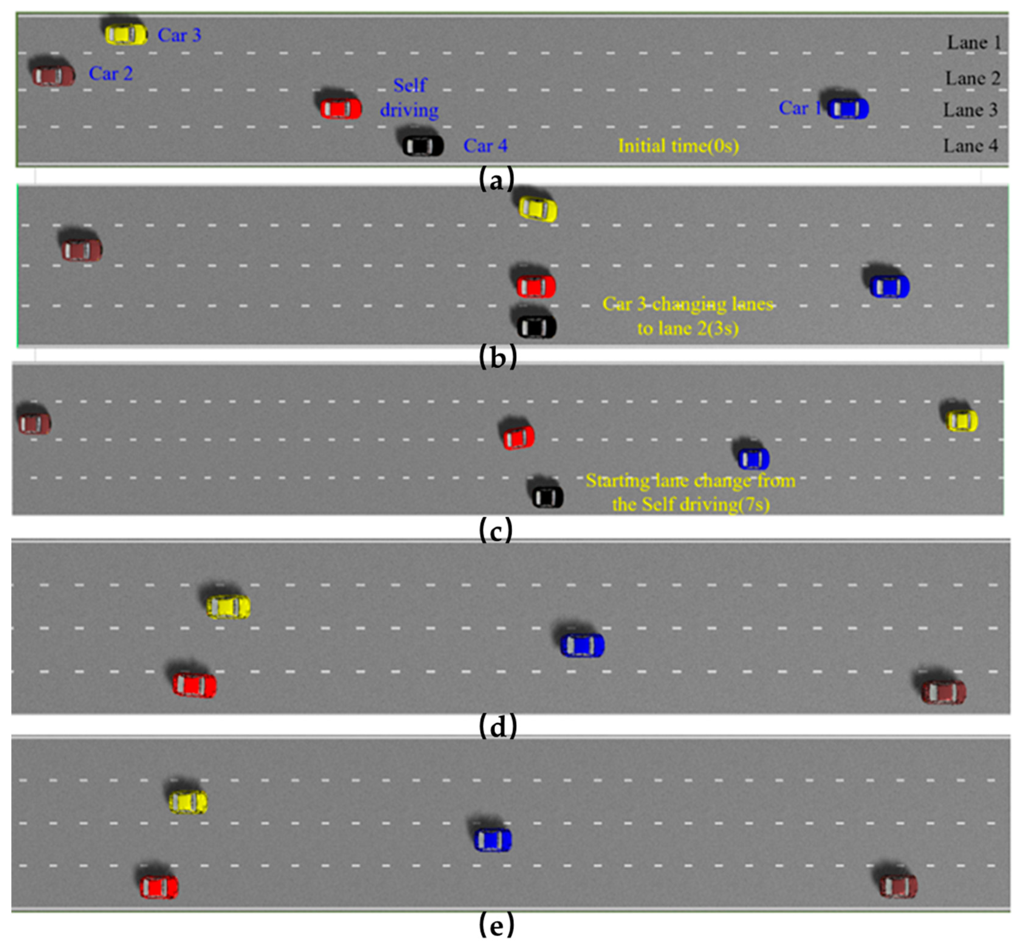
4.4. Slow Lane Change

In this scenario simulation, the vehicle needs to slowly change lanes towards the target lane in the face of traffic conditions such as road narrowing and lane merging. The initial state is shown in Figure 17a, where the longitudinal distance between the self-driving car and car 1 is 80 m and the longitudinal distances between cars 2, 3, 4, and 5 are 40 m, 5 m, 42 m, and 45 m, respectively. The self-driving car and car 2 are travelling at a constant speed of 27 m/s, whereas cars 1, 3, 4, and 5 are travelling at 20 m/s along their current respective lanes. In this scenario, car 2 is set to keep deviating from the lane centerline until 4 s, when it starts to change lanes into lane 2, as shown in Figure 17b. The intermediate process of lane change is shown in Figure 17c,d. According to Figure 17e, the main car completed the entire lane change process.
Figure 18a,d shows that in the initial state, the longitudinal distance between the car and cars 5 and 3 is at a dangerous distance, resulting in a safety level of 1 for the adjacent lanes 2 and 3 with respect to the car. At an amount of time of 2 s into the journey, the longitudinal distance between the car and cars 5 and 1 is greater than the minimum safety distance Dsafe, whereas the safety level of lane 1 on the left of the car is raised to 3 due to car 2 deviating from the lane and the safety level of the lane on the right is 3. Therefore, the decision level determines that it cannot overtake the car and the car brakes to slow down. Car 2 completes the lane change into lane 2 at the 4th second, at which point the safety level on the left side of the car reverts to 1. The car cruises until the 10th second with the front car’s speed as the reference speed, at which point the right lane meets the lane-change condition and the safety level is raised to 4, whereas the safety level on the left side continues to remain at 1 due to car 2.
Figure 18b shows the trajectory of the self-driving car and two vehicles. It can be seen that even though the left lane of the self-driving car has room for a lane change, the self-driving car makes the decision to change lanes to the right to avoid the hazard due to the presence of vehicles in the second adjacent lane on the left carrying out abnormal movements. This shows that the designed lane-change decision method has higher safety in cases where there is a change in the lateral movement status of an associated vehicle in the second adjacent lane.

5. Conclusions

In this paper, a lane-change decision architecture is proposed, consisting of three modules: “intention generation → feasibility judgment → lane change decision generation”, and the logical relationships between them are explained. The traffic environment around the vehicle is pre-processed and zoned, and the movements of vehicles in the second to adjacent lane are taken into account to ensure the vehicle’s safety during travel. Intent generation and feasibility judgment conditions are used as state transfer conditions using a state machine, and a path-velocity planning method is used to plan the vehicle trajectory. An algorithm for identifying valid targets is designed for a multilane scenario, and a five-polynomial-based algorithm for planning the trajectory of a self-driving vehicle’s lane change is designed based on an optimization approach. An intelligent path-tracking control method is proposed based on considering the lateral stability boundary and lateral stability. The effectiveness of the proposed model prediction controller is verified using an offline simulation platform, and the effectiveness of the speed tracking controller is verified by simulation. The algorithm proposed in this paper was verified using PreScan, CarSim, and Matlab/Simulink simulation software; four simulation scenarios were established, including following the vehicle when the target vehicle ahead does not meet the self-driving car cruise conditions. These scenarios include: when there are no lane-change conditions, high-speed overtaking driving, the impact of the vehicle motion state on the second to adjacent lane on the self-driving car, and a complex traffic environment to verify the motion planning. The effectiveness of motion planning and motion control is verified. The validation results show that the decision layer architecture proposed in this paper can effectively plan and control the vehicle’s lane-changing behavior and ensure the vehicle’s safety and stability in various scenarios.

Author Contributions

Conceptualization and methodology, C.T. and L.P.; formal analysis, L.P. and C.T.; writing—original draft preparation, L.P. and J.X.; supervision, S.F. All authors have read and agreed to the published version of the manuscript.

Funding

This research was funded by The Central University Basic Research Expenses Project—Strategic Emerging Project of China, grant number N2103028.

Institutional Review Board Statement

Not applicable.

Informed Consent Statement

Not applicable.

Data Availability Statement

Not applicable.

Acknowledgments

This research was funded by The Central University Basic Research Expenses Project, grant number N2103028. Thanks for the support of Northeastern University.

Conflicts of Interest

The authors declare no conflict of interest.

References

  1. Corno, M.; Panzani, G.; Roselli, F.; Giorelli, M.; Azzolini, D.; Savaresi, S.M. An LPV Approach to Autonomous Vehicle Path Tracking in the Presence of Steering Actuation Nonlinearities. IEEE Trans. Control Syst. Technol. 2021, 29, 1766–1774. [Google Scholar] [CrossRef]
  2. Gutjahr, B.; Gröll, L.; Werling, M. Lateral Vehicle Trajectory Optimization Using Constrained Linear Time-Varying MPC. IEEE Trans. Intell. Transp. Syst. 2016, 18, 1586–1595. [Google Scholar] [CrossRef]
  3. Nilsson, J.; Brännström, M.; Fredriksson, J.; Coelingh, E. Longitudinal and Lateral Control for Automated Yielding Maneuvers. IEEE Trans. Intell. Transp. Syst. 2016, 17, 1404–1414. [Google Scholar] [CrossRef]
  4. Fan, H.; Zhu, F.; Liu, C.; Zhang, L.; Zhuang, L.; Li, D.; Zhu, W.; Hu, J.; Li, H.; Kong, Q. Baidu Apollo EM Motion Planner. arXiv 2018, arXiv:1807.08048. [Google Scholar]
  5. Mehdi, S.B.; Choe, R.; Hovakimyan, N. Avoiding multiple collisions through trajectory replanning using piecewise Bézier curves. In Proceedings of the 2015 54th IEEE Conference on Decision and Control (CDC), Osaka, Japan, 15–18 December 2015. [Google Scholar]
  6. Zhu, B.; Yan, S.; Zhao, J.; Deng, W. Personalized Lane-Change Assistance System with Driver Behavior Identification. IEEE Trans. Veh. Technol. 2018, 67, 10293–10306. [Google Scholar] [CrossRef]
  7. Schnelle, S.; Wang, J.; Su, H.; Jagacinski, R. A Driver Steering Model with Personalized Desired Path Generation. IEEE Trans. Syst. Man Cybern. Syst. 2017, 47, 111–120. [Google Scholar] [CrossRef]
  8. Zhu, J.; Tasic, I.; Qu, X. Flow-level coordination of connected and autonomous vehicles in multilane freeway ramp merging areas. Multimodal Transp. 2022, 1, 100005. [Google Scholar] [CrossRef]
  9. Duan, X.; Sun, C.; Tian, D.; Zhou, J.; Cao, D. Cooperative Lane-Change Motion Planning for Connected and Automated Vehicle Platoons in Multi-Lane Scenarios. IEEE Trans. Intell. Transp. Syst. 2023, 24, 7073–7091. [Google Scholar] [CrossRef]
  10. Han, X.; Xu, R.; Xia, X.; Sathyan, A.; Guo, Y.; Bujanović, P.; Leslie, E.; Goli, M.; Ma, J. Strategic and tactical decision-making for cooperative vehicle platooning with organized behavior on multi-lane highways. Transp. Res. Part C Emerg. Technol. 2022, 145, 103952. [Google Scholar] [CrossRef]
  11. Balal, E.; Cheu, R.L.; Sarkodie-Gyan, T. A binary decision model for discretionary lane changing move based on fuzzy inference system. Transp. Res. Part C Emerg. Technol. 2016, 67, 47–61. [Google Scholar] [CrossRef]
  12. Yang, L.; Zhan, J.; Shang, W.-L.; Fang, S.; Wu, G.; Zhao, X. Multi-Lane Coordinated Control Strategy of Connected and Automated Vehicles for On-Ramp Merging Area Based on Cooperative Game. IEEE Trans. Intell. Transp. Syst. 2023, 1–14. [Google Scholar] [CrossRef]
  13. Lin, J.-Y.; Tsai, C.-C.; Nguyen, V.-L.; Hwang, R.-H. Coordinated Multi-Platooning Planning for Resolving Sudden Congestion on Multi-Lane Freeways. Appl. Sci. 2022, 12, 8622. [Google Scholar] [CrossRef]
  14. Coppola, A.; Lui, D.G.; Petrillo, A.; Santini, S. Cooperative driving of heterogeneous uncertain nonlinear connected and autonomous vehicles via distributed switching robust PID-like control. Inf. Sci. 2023, 625, 277–298. [Google Scholar] [CrossRef]
  15. Falcone, P.; Borrelli, F.; Asgari, J.; Tseng, H.E.; Hrovat, D. Predictive Active Steering Control for Autonomous Vehicle Systems. IEEE Trans. Control Syst. Technol. 2007, 15, 566–580. [Google Scholar] [CrossRef]
  16. Gu, Z.; Yin, Y.; Li, S.E.; Duan, J.; Zhang, F.; Zheng, S.; Yang, R. Integrated eco-driving automation of intelligent vehicles in multi-lane scenario via model-accelerated reinforcement learning. Transp. Res. Part C Emerg. Technol. 2022, 144, 103863. [Google Scholar] [CrossRef]
  17. Albarella, N.; Lui, D.G.; Petrillo, A.; Santini, S. A Hybrid Deep Reinforcement Learning and Optimal Control Architecture for Autonomous Highway Driving. Energies 2023, 16, 3490. [Google Scholar] [CrossRef]
  18. Ziegler, J.; Bender, P.; Dang, T.; Stiller, C. Trajectory planning for Bertha—A local, continuous method. In Proceedings of the 2014 IEEE Intelligent Vehicles Symposium Proceedings, Dearborn, MI, USA, 8–11 June 2014. [Google Scholar]
  19. Asano, S.; Ishihara, S. Rule-Based Cooperative Lane Change Control to Avoid a Sudden Obstacle in a Multi-Lane Road. In Proceedings of the 2022 IEEE 95th Vehicular Technology Conference: (VTC2022-Spring), Helsinki, Finland, 19–22 June 2022; pp. 1–7. [Google Scholar] [CrossRef]
  20. You, F.; Zhang, R.; Lie, G.; Wang, H.; Wen, H.; Xu, J. Trajectory planning and tracking control for autonomous lane change maneuver based on the cooperative vehicle infrastructure system. Expert Syst. Appl. 2015, 42, 5932–5946. [Google Scholar] [CrossRef]
  21. Amer, N.H.; Zamzuri, H.; Hudha, K.; Kadir, Z.A. Modelling and control strategies in path tracking control for autonomous ground vehicles: A review of state of the art and challenges. J. Intell. Robot. Syst. 2017, 86, 225–254. [Google Scholar] [CrossRef]
  22. Alcala, E.; Puig, V.; Quevedo, J.; Escobet, T.; Comasolivas, R. Autonomous vehicle control using a kinematic Lyapunov-based technique with LQR-LMI tuning. Control Eng. Pract. 2018, 73, 1–12. [Google Scholar] [CrossRef]
  23. Zadeh, A.G.; Fahim, A.; El-Gindy, M. Neural network and fuzzy logic applications to vehicle systems: Literature survey. Int. J. Veh. Des. 1997, 18, 132–193. [Google Scholar]
Figure 1. Fuzzy System Inference Diagram for Lane-Change Intention.
Machines 11 00820 g001
Figure 2. Vehicle Relations with Surrounding Vehicles. (purple represents the current vehicle, blue represents the same lane vehicle, red represents adjacent lane vehicles, and yellow represents adjacent second lane vehicles. The vehicle to the left of the red dotted line is after the longitudinal position of the main car. For the convenience of illustration, the vehicle is marked and its designation is shown in the figure.)
Machines 11 00820 g002
Figure 3. Adjacent Lane and Vehicle Situational Classification.
Machines 11 00820 g003
Figure 4. Vehicle driving logic and state machine.
Machines 11 00820 g004
Figure 5. Intelligent vehicle trajectory planning.
Machines 11 00820 g005
Figure 6. Vehicle dynamics model.
Machines 11 00820 g006
Figure 7. Phase plan under different front wheel angles, which are (a) 0 rad, (b) 0.12 rad, (c) 0.20 rad and (d) 0.31 rad.
Machines 11 00820 g007
Figure 8. Stability boundary under different front wheel angles, which are (a) 0 rad, (b) 0.12 rad, (c) 0.20 rad and (d) 0.31 rad, at 98 km/h.
Machines 11 00820 g008
Figure 9. The framework of the path-tracking controller for driverless vehicles.
Machines 11 00820 g009
Figure 10. Co-simulation framework.
Machines 11 00820 g010
Figure 11. Follow the driving conditions. The subfigure (a) donates the initial status of the simulation results. The subfigure (b) donates the intermediate process of the simulation results. The subfigure (c) donates the end status of the simulation results.
Machines 11 00820 g011
Figure 12. Simulation results for following the driving conditions. The subfigures (ae) donate the change of intention, safety rating, relative longitudinal distance, velocity and acceleration, respectively.
Machines 11 00820 g012
Figure 13. Constant speed lane change condition. The subfigure (a) donates the initial status of the simulation results. The subfigures (b,c) donate the intermediate process of the simulation results. The subfigure (d) donates the end status of the simulation results.
Machines 11 00820 g013
Figure 14. Simulation results for the constant speed lane change conditions. Simulation results for constant speed lane change conditions have been given as Figure 14. The subfigures (ae) donate the change of intention, safety rating, relative longitudinal distance, lateral position and yaw angel and yaw rate, respectively.
Machines 11 00820 g014
Figure 15. Simultaneous lane change condition. The subfigure (a) donates the initial status of the simulation results. The subfigures (b,c) donate the intermediate process of the simulation results. The subfigure (d) donates the end status of the simulation results.
Machines 11 00820 g015
Figure 16. Simulation results for simultaneous lane change conditions. Simulation results for simultaneous lane change conditions have been given as Figure 16. The subfigures (ae) donate the change of intention, safety rating, relative longitudinal distance, velocity and lateral position, respectively.
Machines 11 00820 g016
Figure 17. Slow lane change conditions. The subfigure (a) donates the initial status of the simulation results. The subfigures (bd) donate the intermediate process of the simulation results. The subfigure (e) donates the end status of the simulation results.
Machines 11 00820 g017
Figure 18. Simulation results of slow lane change conditions. Simulation results for slow lane change conditions have been given as Figure 18. The subfigures (ae) donate the change of intention, safety rating, relative longitudinal distance, velocity and lateral position, respectively.
Machines 11 00820 g018
Table 1. Fuzzy rule table.
ψDNBNMNSZOPSPMPB
ψv
NBNSNSNMNMNBNBNB
NMNSNSNMNMNMNBNB
NSZOZONSNSNSNMNM
ZOPMPMPSPSZONSNM
PSPMPMPSPSZOZONS
PMPBPBPMPMPSZONS
PBPBPBPBPMPMPSPS
Table 2. Vehicle Lane-Change Decision Based on Fuzzy Inference System.
Lane-Changing Willingness Value (ψh)Vehicle Lane-Changing Decision
0.71 < ψh ≤ 0.51no lane change
0.51 < ψh ≤ 0.71waiting for lane change
0.71 < ψh ≤ 1.00executing lane change
Table 3. The correction factor.
FactorCorrection FactorThe Range of Real Factor Value
Rainqrain ∈ [0, 1, 2, 3]0~50 (mm/h)
Windqwind ∈ [0, 1, 2, 3]0~12 (Beaufort scale)
Fogqfog ∈ [0, 1, 2, 3]0~6.2 (mile)
Roadqroad ∈ [0, 1, 2, 3]Dry/Damp/Stagnant water/Snow and ice cover/Muddy
Disclaimer/Publisher’s Note: The statements, opinions and data contained in all publications are solely those of the individual author(s) and contributor(s) and not of MDPI and/or the editor(s). MDPI and/or the editor(s) disclaim responsibility for any injury to people or property resulting from any ideas, methods, instructions or products referred to in the content.

