Optimization of a 6-DOF Platform for Simulators Based on an Analysis of Structural and Force Parameters

Abstract

Automotive driving simulators are widely used in driving schools and training centers, where they help students acquire the necessary skills without risk to life and health. This paper presents modern research in the field of creating a model and a real prototype of an automotive driving simulator based on the Gough–Stewart platform. This investigation presents optimized geometric parameters using the PSO algorithm. Virtual prototypes of the robotic platform were created by MSC Adams. In turn, this made it possible to conduct the simulation of kinematic and dynamic parameters. They represent operating conditions when exposed to workloads. This paper shows a prototype of an automotive driving simulator and special equipment with an integrated system of virtual 3D models of real terrain.

1. Introduction

Professional driving simulators are widely used in driving schools and training centers, where they help students acquire the necessary skills without risk to life and health. In addition, driving simulators are used to train professional drivers who have to drive complex vehicles such as trucks, buses, trams, etc. All driving simulators are classified as professional, which are very technically complex and are used in driving schools, or home, which can be used on a laptop. The development of professional driving simulators is a complex task that can be solved in various ways. To create a more realistic driving experience, virtual and augmented reality (VR) systems are often used using neural network algorithms. With such systems, it is possible to create a fully interactive environment that allows students to have a more realistic driving experience. For example, when using VR, a student can see on the simulator screen not only a road and a car, but also other vehicles, pedestrians, traffic signs, etc. Also, VR can be used to simulate different climate conditions that can affect the driving [1,2,3]. Another direction is the creation of a physical environment for the driver, which recreates the cab of a real vehicle with all of the controls [4,5]. Driving simulator cabs can be created as both stationary and portable. They can be installed in driving schools, training grounds, or other places where driving is taught. One example of driving simulator cockpits is Cruden’s “Driver-in-Motion” project. This cab is equipped with a realistic driving system that allows students to have a more realistic driving experience. Stationary simulators cannot convey the dynamics of vehicle movement, the absence of which leads to a misunderstanding of the principles of control of aircraft or ground heavy vehicles for civil and military purposes. With mobile training simulators, pilots can simulate a variety of flight scenarios, including takeoff, landing, low-altitude flight, low-visibility flight, and other pitch, roll, and yaw situations. One example of a mobile simulator is the “Full Flight Simulator” project by CAE. This simulator is equipped with a realistic cockpit and can simulate flights on various types of aircraft [6,7,8]. One of the means that can provide the required motion parameters is parallel mechanisms due to such advantages as high rigidity, accuracy, load capacity, and low manufacturing cost. Parallel engines allow for more accurate and realistic flight simulations, which improves the quality of pilot and driver training. In addition, parallel mechanisms provide high accuracy and reliability of simulators, which reduces the likelihood of accidents. One example of a parallel mechanism for exercise equipment is the Moog Hexapod system. This mechanism is equipped with six hydraulic cylinders that provide the platform 6-DOF movement. This allows you to create realistic rolling and shaking effects that occur during flight. The described mechanism is a 6-DOF Gough–Stewart platform. There are many configurations of the Gough–Stewart platform and mechanisms based on it. In each of the configurations, the platform includes six rods of variable length; however, the number of joints of the base and the mobile platform may be different. The article in [9] considers the design of a 6-RUS configuration for a flight simulator and the optimization of geometric parameters, taking into account the physical limitations of the mechanism [10,11,12,13,14,15].

To investigate the operation of parallel manipulators, researchers use various approaches and methods. A number of researchers use an analytical approach to solve direct and inverse problems of kinematics [16,17]. At the same time, the direct task of kinematics, which consists in determining the coordinates of the working body depending on the lengths of the extension of the rods, does not have a clearly formalized solution and requires the use of more complex mathematical methods compared with inverse kinematics—determining the lengths of the extension of the rods according to the given coordinates of the working body, the solution of which in the general case converges to the solution of six nonlinear equations for 6-DOF manipulators of the Gough–Stewart platform, type 6-6. Mathematical approaches used to solve the forward kinematics can be conditionally divided into two groups: the use of the apparatus of vector algebra and analytical geometry.

The functional characteristics of modern software tools open up new opportunities for studying the issues described above. We present some of them that have been studied by the following authors: modeling the geometry and structural configuration of the Gough–Stewart platform in the Mathcad environment [18]; optimization of the angular and linear dimensions of parallel kinematics manipulators using the MATLAB/Simulink, the built-in package with the SimMechanics library for visual modeling of spatial mechanisms, and the highly efficient SQP optimization method [19]; improvement of the pneumatic control system of the Stuart platform based on the Investigation of the dynamic characteristics of the pneumatic drive using the MATLAB/Simulink and AMESim software packages [20]; and modeling of the servo control system of the lever platform.

Stewart solved the inverse kinematics in MATLAB/Simulink using the MATLAB/Simulink library [21], solving the direct and inverse problems of controlling the kinematics of the Stewart platform using MATLAB [22]. As can be seen from the listing, one of the popular software tools is MATLAB. The work presented also uses this package, with a distinctive feature being cosimulation with Adams.

Cosimulation is a powerful tool for designing complex systems and consists in the interconnected use of a complex of specialized software tools. As is known, one of the significant drawbacks of parallel mechanisms is the possibility of interference (crossing) of individual kinematic chains. Cosimulation allows you to perform a dynamic analysis of a system, providing a visual output of the functional parameters in real time and allowing you to check their performance in a virtual prototype.

In this paper, we consider the design of an automotive driving simulator based on the Gough–Stewart platform. An analysis of the existing solutions for an automotive driving simulator based on the Gough–Stewart platform revealed the following:

1.

Most of them are used as flight simulators, as well as for training cosmonauts for manned flights.

2.

To train drivers of ground vehicles, simulators are used on the basis of either three-stage platforms or a stationary platform to simulate a driver’s cab or seat with a virtual display of the vehicle’s movement.

In this regard, there is a problem of creating effective automotive driving simulators that provide simulation of a vehicle in all six coordinates in space, with the possibility of working out the required dynamics of the movement of a real vehicle, taking into account the relief and geography of the real area in the city or beyond. The studies presented in the article are aimed at creating methodological foundations for designing automotive driving simulators based on the Gough–Stewart platform based on modern numerical modeling and CAD/CAM design methods for building digital twins that adequately reflect the properties of real prototypes, as well as designing the prototypes themselves.

2. Requirements for the Automotive Driving Simulator

To create the movement of the simulator cabin for driving a vehicle, various parameters of the movable platform are used. They include the following:

1.

Movement velocity: This parameter determines the velocity of movement of the simulator cabin in accordance with the actions of the driver.

2.

Acceleration and deceleration: These parameters determine how fast the simulator cabin can accelerate and decelerate depending on the actions of the driver.

3.

Tilt angle: This parameter determines the angle of inclination of the simulator cab when turning and changing the direction of movement.

4.

Vibration: This parameter determines the degree of vibration that the simulator cabin experiences when driving on various surfaces.

5.

Suspension height: This parameter determines the height of the treadmill cabin suspension, which allows you to create realistic effects when riding on uneven terrain.

6.

Rigidity factor: This parameter determines the stiffness of the simulator cab suspension, which allows you to create realistic effects when driving on various surfaces.

All these parameters of the moving platform are used to create the most realistic simulation of driving a vehicle in the simulator. They allow the driver to gain experience of riding on different types of roads and in different conditions, which improves the quality of learning and safety on the road. One of the key parameters for the automotive driving simulator is the angle of inclination of the surface. In most countries, it is customary to build roads with a slope of no more than $30\%$, which corresponds to an angle of $17\%$. This value may vary by region and rarely exceeds $20\%$. The feeling of acceleration and braking is very important for the feeling in the car. Assume that the simulation vehicle accelerates to a velocity limit of 60 km/h in 10 seconds; then, to experience smooth braking and acceleration, the platform must provide a minimum acceleration of $1.6$ m/${\mathrm{s}}^2$. It is known that the deceleration of modern road cars with a standard brake system with ABS is on average 1 g or 10 m/${\mathrm{s}}^2$ during emergency braking. Therefore, the maximum platform acceleration must be 10 m/${\mathrm{s}}^2$. The carrying capacity of the platform must ensure the movement of the simulator cabin with the person in it. The final weight of the cabin may vary depending on the type of simulator but should not exceed 500 kg without stock. According to the given parameters, the following requirements were formulated for the mobile platform, which are presented in

Table 1. Technical requirements for the automotive driving simulator.

Options	Values
Range of motion:
Roll	$\pm {20}^{°}$
Pitch	$\pm {20}^{°}$
Z-axis	$\pm 150$ mm
X and Y-axis	$\pm 150$ mm
Linear acceleration	left-right, up-down: 5 m/${\mathrm{s}}^2$
	Forward-backward: 10 m/${\mathrm{s}}^2$
Angular velocity	$1.5$ rad/s
Load capacity	300 kg
Type of drive	Electromechanical
Positioning accuracy	1 mm
Number of dynamic platform drives	6

:

3. Mathematical Model of the Platform

The 6-6 UPU (universal–prismatic–universal) platform is a 6-DOF parallel mechanism. The mechanism itself has 6 kinematic chains (Figure 1), which connect the fixed base to the movable platform through linear actuators ($L_i$) and universal joints at the bases ($A_i$$B_i$). The base and the movable platform are hexagonal figures (in particular cases, a triangle). The required position and orientation of the mobile platform is achieved by changing the length of six rods [23].

The solution of the 6-6 UPU inverse kinematics for the input coordinate $L_1$ is written as

$${\displaystyle L_1={\left({\left(A_{1x}-B_{1x}\right)}^2+{\left(A_{1y}-B_{1y}\right)}^2+{\left(A_{1z}-B_{1z}\right)}^2\right)}^{1/2}}$$

(1)

where $B_{1x}$, $B_{1y}$, $B_{1z}$ is the coordinate of point $B_1$ in the coordinate system $X_1$$Y_1$$Z_1$ of the fixed platform. The values of the other input coordinates are determined similarly. The coordinates of points $B_i$ are defined as

$${\displaystyle {\mathbf{B}}_{\mathbf{i}}={\left(B_{ix}{B}_{iy}{B}_{iz}1\right)}^T=\mathbf{M}·{\left(B_i{x}^{\left(2\right)}{B}_i{y}^{\left(2\right)}{B}_i{z}^{\left(2\right)}1\right)}^T,}$$

(2)

where $B_{1x}^{\left(2\right)},B_{1y}^{\left(2\right)},B_{1z}^{\left(2\right)}$ are the coordinates of $B_i$ points in the $X_2$$Y_2$$Z_2$ coordinate system of the moving platform, and M is the transformation matrix for the transition from a moving to a fixed coordinate system.

It is also necessary to take into account the possibility of singularities. J.P. Merlet, in his work in [24], noted that such a platform occurs when the axis of any of the drive rods hits the plane of the movable platform. From this, it follows that a singularity arises when at least one of the points $A_i$ belongs to the plane of the moving platform. The condition for the occurrence of a singularity can be written in the following form

$${\displaystyle a{A}_{ix}+b{A}_{iy}+c{A}_{iz}+d=0}$$

(3)

where $a,b,c,d$ are the coefficients of the moving platform plane equation, which are defined as

$${\displaystyle a=k_x,b=k_y,c=k_z,d=k_x{O}_{2x}+k_y{O}_{2y}+k_z{O}_{2z},}$$

(4)

Getting into a singularity occurs when the sign of the left side of Equation (3) is changed; therefore, it is necessary to add the condition of its sign constancy

$${\displaystyle a{A}_{ix}+b{A}_{iy}+c{A}_{iz}+d>0}$$

(5)

Let us perform the formulation of the optimization problem for the platform, taking into account the condition of providing the required workspace and minimizing the maximum forces that occur in the drives.

4. Setting the Optimization Problem

4.1. Optimization Parameters

As optimization parameters, we use platform radii $R_1$ and $R_2$, angles of mutual arrangement of joints $\psi$ and $\omega$, and the limit values of rod lengths $L_{min}$ and $L_{max}$.

4.2. Criteria

As a result of optimization, it is necessary to determine the geometric parameters that ensure the compactness of the structure, the forces in the actuators are reduced, and the required workspace is provided. Thus, the objective function can be written as

$${\displaystyle F=F_S+F_W+F_A}$$

(6)

where $F_S$ is a component of the criterion that takes into account the compactness of the design, $F_W$ is a component of the criterion that takes into account the restriction on the required workspace, $F_A$ is a component of the criterion that takes into account the maximum efforts in the actuators.

4.3. Compact Design

Let us write down the component $F_S$ taking into account the compactness of the design as

$${\displaystyle F_S=R_1+R_2+L_{min}+L_{max}+p_1{\vartheta }_1\left(\frac{k_l{L}_{max}}{L_{min}}\right)+p_2\left({\left(\frac{k_R{R}_1}{R_2}\right)}^{2{\vartheta }_2-1}-1\right)\to min}$$

(7)

where $R_1$ is the radius of the fixed platform, $R_2$ is the radius of the fixed platform, $L_{min}$ and $L_{max}$ are the limit values for changing the lengths of the rods, $p_i$ are the given penalty factors, $k_L=0.6$ is the minimum recommended ratio of the minimum and maximum lengths of the rods to ensure sufficient space inside the rod to accommodate the ball–screw pairs, and $k_R=0.7$ is the ratio of platform radii $R_2⁄R_1$, ${\vartheta }_i$ recommended according to [25]—the Heaviside functions:

$${\displaystyle {\vartheta }_1=\left\{\begin{array}{cc}\hfill 1,\mathrm{if}\hfill & \hfill \frac{L_{min}}{L_{max}}<0.6\\ \hfill 0\hfill & \hfill -\mathrm{otherwise}\end{array}\right.,{\vartheta }_2=\left\{\begin{array}{cc}\hfill 1,\mathrm{if}\hfill & \hfill \frac{R_2}{R_1}<0.7\\ \hfill 0\hfill & \hfill -\mathrm{otherwise}\end{array}\right.}$$

(8)

4.4. Workspace

The set A describing the workspace of the platform for the selected parameter values must be guaranteed to include some given area or trajectory in order to ensure the functional purpose of the robot. The required area B can be specified as a 3D geometric figure, such as a box. In this case, we write the component $F_W$, taking into account the required workspace, as

$$F_W=\left|{\vartheta }_3-1\right|\left(f_V+1\right)p_3+{\vartheta }_3\left(p_3+p_4\right)\to min$$

(9)

where, $p_i$ are the specified penalty coefficients, $f_V$ is the estimate of the proportion of the required area that cannot be provided by the platform $(f_V\in [0,1)$; if the overall dimensions of the required area do not exceed the overall dimensions of the workspace of the platform for each of the measurements, $f_V⩾1$ otherwise), ${\vartheta }_3$ is the Heaviside function:

$${\vartheta }_3=\left\{\begin{array}{cc}\hfill 1,\mathrm{if}\hfill & \hfill A=\varnothing \\ \hfill 0\hfill & \hfill -\mathrm{otherwise}\end{array}\right.$$

(10)

The algorithm for determining the estimation of the $f_V$ fraction of the required area that cannot be provided by the platform, as well as the optimization of the platform 6-6 UPU platform for arbitrary parameters, excluding force characteristics considered earlier in the paper [26].

4.5. Force in Actuators

The component $F_A$ corresponds to the maximum of the forces arising in the actuators during the movement of the platform when working out trajectories. To determine the forces in the actuators, we use cosimulation. Cosimulation is carried out using Adams View Student Edition 2022.1, MATLAB R2020a, which makes it possible to compare and analyze various design variants of the manipulator in terms of the possibilities of working out the given trajectories of the movement of the working body, the investigation of force–torque characteristics that occur during movement [27].

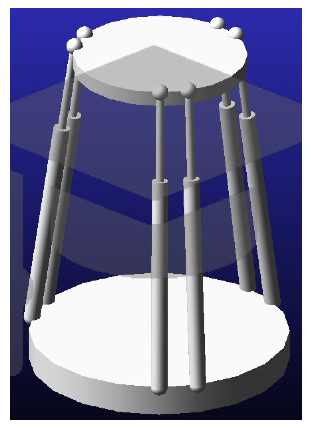
Figure 2 presents an example of a digital layout. The digital layout has the properties of a parameterized model for the purpose of automated changes in design parameters during simulation.

The management of a parameterized model during its automated rebuilding in MSC Adams is implemented through the use of the interface of the high-level general-purpose object-oriented programming language Python, which is used as an alternative to the internal Adams View command language for creating and iteratively changing modeling objects in Adams. The Adams View Student Edition 2022.1, Python 3.8 object-oriented interaction framework is coordinated by mapping each individual entity in Adams to a class in Python that has properties and methods. The use of Python allows you to automate the execution of a series of computational experiments, which consist in sequential multiple changes in geometric parameters, as well as subsequent simulation of the model and analysis of the results in order to find the best design options according to specified criteria. The use of Python significantly increases the efficiency of constructive analysis by reducing labor intensity, increasing the arbitrariness of the enumeration process and the number of possible computational simulations.

For Adams–Python interaction, special procedures and functions have been developed that solve the following main tasks: determining the coordinates of the junction points of electric cylinders with the base and table; creating a hexapod model in AdamsView; changing the geometric parameters of the model; and analyzing the results of a computational experiment and the search for simulations corresponding to the studied geometric parameters of the model according to the specified optimality criteria. To simulate real constructive interfaces of RPP, the following special software operators of the Adams application were used: the base is fixed to ground using FixedJoint, the sleeve is attached to the base using SphericalJoint, and the EC rods are similarly paired with the working surface of the platform. To simulate the movement of an electric cylinder, the sleeve and the rod are connected to each other at the points of contact by a TranslationalJoint interface. As external forces, the force of gravity directed vertically downwards (in the direction of the axis—$OY$) and the payload applied at the point of the center of mass, which is specified in accordance with the requirements of the designed RPP industrial design, are set.

Figure 3 shows the Simulink scheme used to simulate the investigated manipulator: the set of Euler angles is converted into the corresponding rotation matrix in the Euler $X,Y,Z$ block; the inverse kinematics is solved by the block Inverse Kinematics Module, and the required extension lengths of the rods are generated at the output; and in the Saturation block, physical restrictions on the movement of electric cylinders are worked out. A feature of this scheme is the Adams_sub block, exported to MATLAB from Adams, which determines the physical and mechanical parameters of the manipulator through a digital layout created in Adams. The integration of this block provides the Adams View-MATLAB Simulink cosimulation process; for this, the coordinates of the specified trajectory of the movement of the working body, which change in time, are used as input parameters. The point located in the center of the movable platform is taken as the coordinate of the working body. At the output of the Adams_sub block, the actual coordinates of the working body are generated, taking into account the design parameters of the mechanism and its physical and mechanical properties.

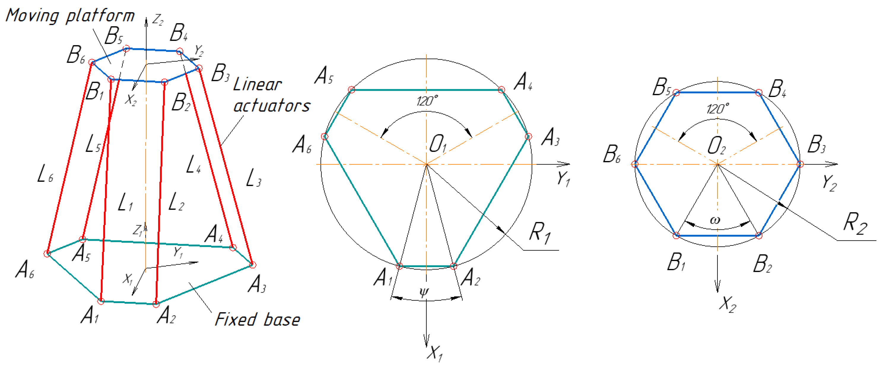
When implementing the simulation, two coordinate systems were used: a global Cartesian coordinate system with the origin at the geometric center of the base and a local relative Cartesian coordinate system with the origin at the geometric center of the working body (movable platform). The input parameters of the system are given by the coordinate vector of the points of the trajectory being worked out as an increment (change) relative to the zero (initial position); that is, a local relative coordinate system is used. The coordinates of the base joints and the coordinates of the initial positions of the joints of the movable platform are given in the global coordinate system. In the initial position, the directions of the axes of the global and local coordinate systems coincide. When the working body moves along a given trajectory, the local coordinate system can turn at certain angles with respect to the global coordinate system. To take this circumstance into account, a generalized rotation (transformation) matrix is used:

$$R_j=\left[\begin{array}{ccc}cos{\beta }_{j}cos{\gamma }_j& -cos{\beta }_{j}sin{\gamma }_j& sin{\beta }_j\\ cos{\gamma }_{j}sin{\beta }_{j}sin{\alpha }_j+cos{\alpha }_{j}sin{\gamma }_j& cos{\alpha }_{j}cos{\gamma }_j-sin{\alpha }_{j}sin{\beta }_{j}sin{\gamma }_j& -sin{\alpha }_{j}cos{\beta }_j\\ sin{\alpha }_{j}sin{\gamma }_j-cos{\alpha }_{j}cos{\gamma }_{j}sin{\beta }_j& cos{\gamma }_{j}sin{\alpha }_j+cos{\alpha }_{j}sin{\beta }_{j}sin{\gamma }_j& cos{\alpha }_{j}cos{\beta }_j\end{array}\right]$$

(11)

where $\alpha ,\beta ,\gamma$ are the Euler angles, respectively, the angles between the abscissa, ordinate, and applicate axes of the two accepted coordinate systems; j is the number of points of the investigated trajectory of the movement of the working body. Cartesian coordinates of the trajectory of the movement of the working body are given in the local system by the vector

$$d_j=\left[\begin{array}{ccc}\hfill d_{xj}\hfill & \hfill d_{yj}\hfill & \hfill d_{zj}\hfill \end{array}\right]$$

(12)

where j is the number of points of the investigated trajectory of the movement of the working body; the initial coordinates of the joints fixed on the movable platform are given by the matrix

$$P=\left[\begin{array}{cccccc}\hfill P_{1x}\hfill & \hfill P_{2x}\hfill & \hfill P_{3x}\hfill & \hfill P_{4x}\hfill & \hfill P_{5x}\hfill & \hfill P_{6x}\hfill \\ \hfill P_{1y}\hfill & \hfill P_{2y}\hfill & \hfill P_{3y}\hfill & \hfill P_{4y}\hfill & \hfill P_{5y}\hfill & \hfill P_{6y}\hfill \\ \hfill P_{1z}\hfill & \hfill P_{2z}\hfill & \hfill P_{3z}\hfill & \hfill P_{4z}\hfill & \hfill P_{5z}\hfill & \hfill P_{6z}\hfill \end{array}\right]$$

(13)

where $P_{ix},P_{iy},P_{iz}$ are the Cartesian coordinates of the i-th joint in the global coordinate system; the coordinates of the joints fixed on the base are given by the matrix

$$B=\left[\begin{array}{cccccc}\hfill B_{1x}\hfill & \hfill B_{2x}\hfill & \hfill B_{3x}\hfill & \hfill B_{4x}\hfill & \hfill B_{5x}\hfill & \hfill B_{6x}\hfill \\ \hfill B_{1y}\hfill & \hfill B_{2y}\hfill & \hfill B_{3y}\hfill & \hfill B_{4y}\hfill & \hfill B_{5y}\hfill & \hfill B_{6y}\hfill \\ \hfill B_{1z}\hfill & \hfill B_{2z}\hfill & \hfill B_{3z}\hfill & \hfill B_{4z}\hfill & \hfill B_{5z}\hfill & \hfill B_{6z}\hfill \end{array}\right]$$

(14)

where $B_{ix},B_{iy},B_{iz}$ are the Cartesian coordinates of the i-th joint in the global coordinate system; the coordinates of the joints fixed on the movable platform, when working out a given trajectory of the working body, are given by the matrix

$$A_l=\left[\begin{array}{cccccc}\hfill A_{1xj}\hfill & \hfill A_{2xj}\hfill & \hfill A_{3xj}\hfill & \hfill A_{4xj}\hfill & \hfill A_{5xj}\hfill & \hfill A_{6xj}\hfill \\ \hfill A_{1yj}\hfill & \hfill A_{2yj}\hfill & \hfill A_{3yj}\hfill & \hfill A_{4yj}\hfill & \hfill A_{5yj}\hfill & \hfill A_{6yj}\hfill \\ \hfill A_{1zj}\hfill & \hfill A_{2zj}\hfill & \hfill A_{3zj}\hfill & \hfill A_{4zj}\hfill & \hfill A_{5zj}\hfill & \hfill A_{6zj}\hfill \end{array}\right]$$

(15)

where $A_{ixj},A_{iyj},A_{izj}$ are the Cartesian coordinates of the i-th joint for the j-th point of the investigated trajectory of the movement of the working body.

When solving the inverse kinematics problem to determine the required values for the extension of the rods corresponding to the given coordinate of the working body when moving along the required trajectory, the required coordinates of the joints of the movable platform are first determined:

$$A_j=D_j+R_j·P-B$$

(16)

where the matrix $D_j$ is obtained by concatenating the vector $d_j$ to reduce it to [$3\times 6$]. The matrix $A_j$ is inversely concatenated to obtain $six[1\times 3]$ vectors containing the Cartesian coordinates of the joint positions. For each vector, the scalar product operation is performed

$$∥v_i∥=\sqrt{{\overrightarrow{v}}_i·{\overrightarrow{v}}_i}$$

(17)

The obtained values $∥v_i∥$ are written by concatenation into the matrix $JP$ (Joint Position) with dimension $[1\times 6]$ The Repmat built-in function creates a $[1\times 6]$$NL$ (Nominal Length) matrix: repmat ($A,n$) returns an array containing n copies of A in row and column dimensions, using the initial height of the platform you specify. At the final step, we obtain the $NP$ (New Position) extension length matrix by subtracting $NL$ from $JP$:

$$NP=NL-JP$$

(18)

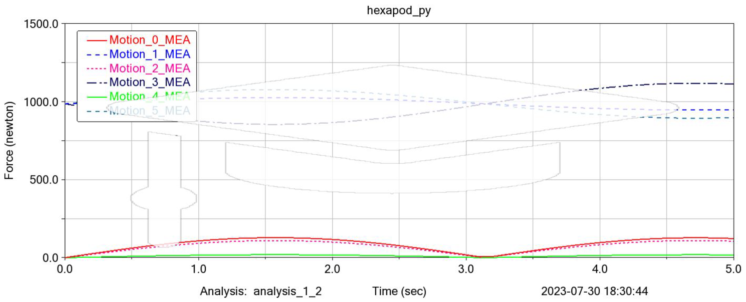
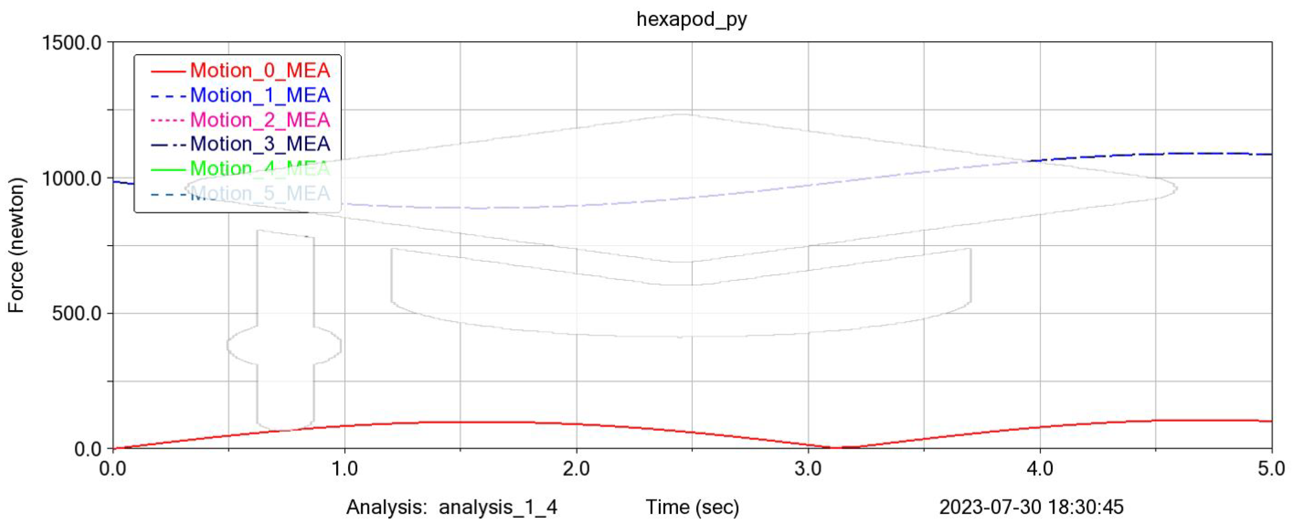
The Adams_sub block includes the MSC Software block, in the settings of which it is possible to change the simulation type: from usual calculated to interactive (Figure 4 and Figure 5). In this case, when the simulation starts, the Adams window opens and the motion of the system is visualized in the simulation time mode.

4.6. Optimization Software Package

The particle swarm algorithm is used as an optimization method. Particle swarm optimization (PSO) is a widely used two-component method of evolutionary optimization based on swarm [28]. The particle swarm algorithm solves the problem by having a set of potential solutions, called particles, and moving these particles in the search space according to a simple mathematical formula depending on the position and velocity of the particle. The movement of each particle depends on its local best-known position but is also directed to the best-known positions in the search space, which are updated as other particles find better positions. It is expected that this will lead to the transition of the swarm to better solutions.

The optimization algorithm using the PSO method is implemented in the C++ programming language. To integrate the developed software package with the calculation module of the $F_A$ component using ADAMS, data exchange modules via JSON files are implemented:

-

Flag file that takes three values: 0 (Optimization Software package is waiting, Adams is running), 1 (Adams is waiting, optimization software package is running), and 2 (optimization is completed).

-

A file with parameters to which the optimization software package writes and from which Adams reads data for simulation.

-

A file with the Adams simulation results.

Let us perform a computational experiment in accordance with the requirements for the training complex (Table 1).

5. Optimization Results

Assign the initial platform data and algorithm optimization parameters. Working area approximation accuracy $\delta =50$ mm. Platform orientation ii angle range $\alpha \in [-{20}^{°};{20}^{°}]$, $\beta \in [-{20}^{°};{20}^{°}]$, $\gamma \in [-{20}^{°};{20}^{°}]$. Ranges of optimization parameters: $\psi \in [{10}^{°};{110}^{°}]$, $\omega \in [{10}^{°};{110}^{°}]$, $R_1\in [300;1000]$, $R_2\in [300;800]$, $L_{min}\in [500;1500]$, $L_{max}\in [800;2000]$, $p_1=10000$, $p_2=3000$, $p_3=5000$, $p_4=10000$. The dimensions of the required area are 300 × 300 × 300 mm. The parameters of the PSO algorithm: number of individuals in the initial population $H=40$, number of generations $W=10$, number of groups $G=2$, and values of free parameters ${\alpha }_{PSO}=0.7,{\beta }_{PSO}=1.4,{\gamma }_{PSO}=1.4$. The simulation results are presented in

Table 2. Optimization results.

No	${\mathit{R}}_1$	${\mathit{R}}_2$	$\mathit{\psi }$	$\mathit{\omega }$	${\mathit{L}}_{min}$	${\mathit{L}}_{max}$	${\mathit{F}}^{\prime }$
1	410.83	300.00	31.021	102.3954	816.81	1437.46	4407.519
2	427.95	300.00	88.1646	59.8646	582.24	1187.50	5165.164
3	422.33	300.00	64.4136	110	841.56	1485.99	4705.601
4	428.18	300.00	45.7356	10	918.67	1566.89	4810.621
5	432.33	300.00	95.2828	43.5364	703.86	1318.03	4541.053
6	422.00	300.00	110	61.2266	606.11	1239.60	4707.358
7	427.36	300.00	95.9836	10.47626	892.48	1537.11	4463.11
8	397.77	300.00	110	58.4352	690.26	1313.59	4813.845
9	428.35	300.00	10	66.5934	829.66	1475.83	4481.593
10	412.22	300.00	10	106.0262	946.21	1581.95	4483.961
Average	420.9305	300	66.06012	62.85541	782.7866	1414.395	4593.186

.

The best value of the criterion function was obtained as a result of test No. 1. Typical platform movements were used as variants of the specified types of movement: translational vertical, translational longitudinal, translational lateral, rotational relative to the vertical axis (yaw), rotational relative to the horizontal axis (roll), and rotational movement—pitch. When performing a computational simulation of typical movements, the periodic sine function was adopted as a function characterizing the trajectory in time.

Table 3. Averaged forces in actuators for configuration.

Typical Platform Movements
No	Vertical	Longitudinal	Lateral	Pitch	Yaw	Roll
1	1113.913519	1118.200734	1118.200734	1122.228604	1090.06293	1068.616117
2	1137.968532	1612.597737	1612.597737	1459.223941	1432.369034	2004.973753
3	1101.38261	1323.772902	1323.772902	1277.481789	1221.862417	1409.361263
4	1090.1399	1511.971489	1511.971489	1486.820184	1387.518486	1482.974767
5	1124.21538	1193.578113	1193.578113	1134.89315	1147.098345	1364.713017
6	1137.840009	1208.075118	1208.075118	1131.688866	1152.748025	1426.677757
7	1111.120241	1091.807567	1091.807567	1061.394061	1067.360589	1181.28907
8	1121.668392	1208.29001	1208.29001	1130.325378	1156.116529	1432.795168
9	1105.119262	1188.758689	1188.758689	1219.172991	1142.618837	1026.333806
10	1113.390974	1062.198385	1062.198385	1073.171068	1056.825495	1000.901359

presents the average values of the forces in the actuators for six typical movements for ten design variants of the manipulator and

Table 4. Maximum forces in actuators for configuration.

Typical Platform Movements
No	Vertical	Longitudinal	Lateral	Pitch	Yaw	Roll
1	528.0477209	215,246.3	215,246.3	229,930.7	-	110,809.63
2	2922.76	215,246.3	215,246.3	229,930.7	-	110,809.63
3	26,913.48	39,645.25	39,645.25	37,349.03	35,797.46	39,331.24
4	2911.03	50,185.8	50,185.8	45,937.64	49,663.82	55,609.32
5	2922.05	9708.06	9708.06	7891.6	7482.27	14,725.25
6	2915.309	15,763.83	15,763.83	17,191.68	13,502.57	7291.54
7	2918.39	56,005.47	56,005.47	38,043.6	40,718.09	146,270.99
8	2911.91	-	-	-	-	-
9	2921.28	13,227.64	13,227.64	11,008.51	10,148.6	18,925.54
10	2920.09	25,488.29	25,488.29	28,657.46	23,560.66	8027.51

the maximum values in the actuators for the same driving conditions and design options.

The graphical dependences of force characteristics for typical movements are shown in Figure 4, Figure 5, Figure 6, Figure 7, Figure 8 and Figure 9.

The above-described cosimulation tools are used for a comparative analysis of alternative design parameters of the manipulator (Table 1), taking into account the minimization of maximum and average efforts. Typical platform movements were used as variants of the specified types of movement: translational vertical, translational longitudinal, translational lateral, rotational relative to the vertical axis (yaw), rotational relative to the horizontal axis (roll), and rotational movement—pitch. When performing a computational simulation of typical movements, the periodic sine function was used as a function that characterizes the trajectory in time. The averaged and maximum values of the forces in the actuators needed to carry out movement under load were analyzed. All force characteristics were determined for individual typical movements, as well as for each actuator in this movement. When simulating a certain movement, the forces in the actuators were determined in time increments in the period of one complete cycle, the values obtained were averaged for each actuator separately; then, the averaged values obtained for the actuators were averaged for the entire construction. This algorithm was performed for all design options and allowed for a qualitative comparative assessment. For a more complete comparative analysis, the maximum forces arising in the actuators during the development of typical movements were also determined. The maximum values of the forces arising in individual actuators were averaged for the investigation design variant.

Table 5. Amplitude velocities.

Typical Platform Movements
No	Vertical	Longitudinal	Lateral	Pitch	Yaw	Roll
1	1398.272	65,402.05	65,402.05	60,881.23	0	38,692.51432
2	1398.272	65,402.05	65,402.05	60,881.23	0	38,692.51432
3	1389.804	16,680.74	16,680.74	15,222.49	19,062.21	16,061.29617
4	1387.645	20,962.21	20,962.21	18,788.36	25,937.13	21,784.07242
5	1396.642	3483.912	3483.912	2679.171	3042.115	5419.357397
6	1391.116	5942.986	5942.986	6412.494	6532.407	2506.663968
7	1394.234	21,047.49	21,047.49	14,520.02	21,821.75	38,185.18225
8	1388.601	0	0	0	0	0
9	1396.331	5042.327	5042.327	3902.939	4578.547	7269.384542
10	1395.657	10,219.02	10,219.02	11,438.46	12,393.76	2817.450833

and

Table 6. Amplitude accelerations.

Typical Platform Movements
No	Vertical	Longitudinal	Lateral	Pitch	Yaw	Roll
1	0.277199	0.354188	0.373028	0.373073	0	0.222893066
2	0.277199	0.354188	0.373028	0.373073	0	0.222893066
3	0.276564	0.202464	0.192726	0.177762	0.068666	0.202065984
4	0.276405	0.203079	0.203079	0.197338	0.087215	0.202128609
5	0.277	0.098859	0.080875	0.054904	0.009659	0.159716237
6	0.276636	0.113755	0.113755	0.120003	0.018689	0.072813739
7	0.276894	0.207743	0.195081	0.159134	0.077596	0.398102111
8	0.276489	0	0	0	0	0
9	0.277007	0.099436	0.099436	0.073949	0.013535	0.174604933
10	0.27699	0.144958	0.144958	0.160646	0.04601	0.058034849

show the amplitude velocities and accelerations.

Based on the results obtained, digital twin and a prototype simulator are developed.

6. Digital Twin of the Automotive Driving Simulator

Detailed design was carried out for the selected configuration option (Figure 10). In accordance with ISO 15241-2014, universal joint bearings were selected, and their digital twins were built in accordance with the presented dimensions. Using the obtained limit load data, standard actuators with a power of $1.6$ kW each were selected [29]. Detailed digital models of the actuators were obtained from the manufacturer. Thus, in accordance with the optimization performed, the mounting points of the actuators were determined and the platform frame was built. The design of the automotive driving simulator cabin was developed on the basis of the existing design solutions of the proposed prototype manufacturer.

The automotive driving simulator consists of an upper platform 1 and a base 2, which are connected by translational electric drives 3. Each of the translational electric drives 3 is connected to the upper platform 1 and base 2 by cardan joints 4, which are used in the automotive industry and have specifications describing the maximum load. The base has six additional stops 5, each of which is equipped with a vibration support 6. The user’s cab has controls that repeat the controls of the car.

The basis for fixing all the elements is the cab body 7, on which the steering wheel 8 and pedals 9 are fixed, which are a commercially available attachment with a USB connection interface. The digital instrument panel 9 displays information such as RPM, speed, turn signals, and “Check Engine”, the presence of which allows you to determine that the machine is muffled or malfunctioning. Gear shifting is carried out by the electronic selector of the gearbox 10. The simulation image is displayed on the installed monitors 11, which can be performed as a single screen or a series of screens of a smaller diagonal. The landing of the user is carried out due to the adjustable seat 12 with a built-in seat belt, which is necessary to simulate the operating conditions of the car and for safety when driving the simulator.

The control is carried out from the platform control unit containing six frequency converters and six inverter control panels. The platform control unit is connected to the computer via a USB-to-CAN converter. To unblock the platform and block it (including emergency), the platform blocking panel located on the platform operator’s table is used. For the interaction and immersion of the driver in the simulation environment, the software and hardware system “Route” was developed with the following functionality:

-

Automated formation of a digital terrain model (including areas of urban development) based on electronic topographic maps, libraries of three-dimensional objects, results of laser scanning of real terrain, and data from mobile complexes with precision navigation equipment;

-

Creation of new three-dimensional objects;

-

Setting up a behavioral model of dynamic objects (intelligent agents), developed using the principles of multiagent systems;

-

Creation of sets of exercises with various emergency situations for trainees.

7. Laboratory Testing of the Prototype

In accordance with the digital twin of the platform, a prototype of the automotive driving simulator with an integrated system of virtual 3D models of real terrain was built. The prototype of the automotive driving simulator consists of a simulator and an operator console. The operator’s console allows you to launch a dynamic platform, set a map of the area, install a virtual driver’s car at a given point on the map, and track violations when passing a section.

To test the simulator, several tracks with different surface slopes were selected. In accordance with the inclination of the virtual model, the roll and pitch changes of the dynamic platform were compared. Figure 11 shows the passage of a railway crossing with the display of the car on the operator’s console and the movement of the simulator complex at the same time. The turn of the platform is comparable to the movement of the car in the simulation, while for greater realism, there is a linear movement back when entering and forward when exiting.

There are situations in the simulation where movement involves more inclination than the platform specifications allow. This may be dangerous to the operator and cause damage to the equipment. Therefore, the coordinates and rotation angles transmitted to the control module are limited in accordance with the technical requirements of the platform. If the vehicle leans more than 20 degrees in the simulation, the control algorithms limit the platform rotation to a maximum of 20 degrees. Other tests of the platform were aimed at achieving the maximum speed of the platform. To perform this, with the help of the instructor’s console, a simulation of the fall of the car from a state of rest was made. As a result, the platform actuators reached their maximum speed. It is impossible to achieve high speed with the help of simulation due to the established limitation.

Test drives were carried out in the simulation of the polygon, in which there are obstacles of varying complexity, such as a slide (Figure 12a,b). Figure 12c,d shows the test drives on the road in the city simulation. A simulation of the flow of traffic is played in the city, in which the movement of cars occurs at different speeds. If the vehicle remains stationary, other road users will try to avoid the obstacle. Installed traffic lights regulate the order of passage of the intersection. If you violate the rules of the road, the car may get into a traffic accident.

On the first screen (Figure 13a), the instructor displays information about the trainee’s movement with a third-person view; on the second screen (Figure 13b), the testee’s dashboard, route map, and platform control window are displayed.

Figure 14 and Figure 15 show the accelerations that occur when testing test trajectories on an experimental sample. The data are taken from a three-axis accelerometer and a three-axis gyroscope. The accelerations obtained on the experimental sample are comparable to the accelerations obtained as a result of modeling in the Adams environment.

8. Conclusions

The resulting mathematical model, created on the basis of evolutionary algorithms (PSO algorithm), allowed us to solve the problem of optimizing the geometric parameters of the Gough–Stewart platform, taking into account the minimization of dimensions and restrictions on the required workspace and singularities of the platform. The presented technique of the cosimulation of the movement of a parallel manipulator through the integrated application of MATLAB Simulink and Adams View in order to analyze the design options of the manipulator when moving along a given trajectory shows good results and can be used when performing kinematic, dynamic, and force analysis of the mechanism, taking into account its design features through the use of a virtual prototype. This technique allows you to analyze the constructive possibility of working out a given trajectory, evaluating the force characteristics. The presented approach is applicable in the framework of the development, modernization, and optimization of structural elements of parallel manipulators and the definition of the working area, as well as the development of motion control systems. A digital twin of the simulator complex of vehicle management training based on the Gough–Stewart platform with the help of computer-aided design systems has been created. A prototype of the automotive driving simulator was made and tests were carried out. The complex is equipped with a system of virtual 3D models of real terrain using the software and hardware complex “Route”. The experimental studies of the prototype allowed us to evaluate its capabilities and characteristics and adjust the algorithms. Training inexperienced drivers to drive on high-traffic roads is a difficult and dangerous task; in large cities, trainers often resort to using simulators. This allows you to gain basic knowledge of the behavior of various road situations without risking your life. In this light, the development of high-tech robotic devices, such as an automotive driving simulator for vehicle management based on the Gough–Stewart platform, is more relevant than ever.

References

1. Ribeiro, P.R.; Andre, M.; Philipp, K.; Karel, K.A. VR Truck Docking Simulator Platform for Developing Personalized Driver Assistance. Appl. Sci. 2021, 11, 8911. [Google Scholar] [CrossRef]
2. Andres, E.G.; Tiago, K.S.; Carlos, M.M.; Arthur, M.N. Driving Simulator Platform for Development and Evaluation of Safety and Emergency Systems; Cornelll University Library: Ithaca, NY, USA, 2018. [Google Scholar]
3. Valentino, K.; Kevin, K.; Singgih, J.; Endra, D. Dynamic Models Based Virtual Reality Flight Simulator. Internetworking Indones. J. 2022, 11, 23–28. [Google Scholar]
4. Akulov, A.S.; Zheleznov, K.I.; Zabolotny, A.M.; Chabanyuk, E.V. Simulator for training mining locomotive drivers. Min.-Geol.-Pet. Eng. Bull. 2022, 37, 27–35. [Google Scholar]
5. Schmieder, H.; Nagel, K.; Schoener, H. Enhancing a Driving Simulator with a 3D-Stereo Projection System. In Proceedings of the Driving Simulation Conference—DSC 2017, Stuttgart, Germany, 6–8 September 2017. [Google Scholar]
6. Chen, G.; Dian, L.; Huan, C.; Haibo, C. Design and Kinematic Analysis of a Novel Flight Simulator Mechanism. In Proceedings of the 7th International Conference on Intelligent Robotics and Applications, Guangzhou, China, 17–20 December 2014. [Google Scholar]
7. Zhou, X.B.; Fan, M.Y.; Chen, X. Design and Implementation of Instructors Operating Station for Flight Simulator. (Article) 2012. Available online: https://www.researchgate.net/publication/290524149_Design_and_implementation_of_instructors_operating_station_for_flight_simulator (accessed on 10 June 2023).
8. Obaid, M.S.; Mebayet, S. Drone controlled real live flight simulator. J. Phys. 2021, 1818, 121104. [Google Scholar] [CrossRef]
9. Gao, S.; Lei, D.; Liao, Q.; Zhang, G. Generalized Stewart-Gough platforms and their direct kinematics. IEEE Trans. Robot. 2005, 21, 141–151. [Google Scholar]
10. Landman, A.; Hoed, A.; Baelen, D.; Stroosma, O. A Procedure for Inducing the Leans Illusion in a Hexapod Motion Simulator. In Proceedings of the AIAA Scitech 2021 Forum, Virtual Event, 11–15 & 19–21 January 2021. [Google Scholar]
11. Rafał, N.; Bibianna, B.; Piotr, F. Susceptibility to Flight Simulator-Induced Spatial Disorientation in Pilots and Non-Pilots. Int. J. Aviat. Psychol. 2020, 30, 25–37. [Google Scholar]
12. Hoed, A.; Landmann, A.; Baelen, D.; Stroosma, O. Leans Illusion in Hexapod Simulator Facilitates Erroneous Responses to Artificial Horizon in Airline Pilots. Hum. Factors J. Hum. Factors Ergon. Soc. 2020, 64, 962–972. [Google Scholar] [CrossRef]
13. Marinus, B.D.; Zaal, P.M.; Piters, M.; Stroosma, O. Between-Simulator Comparison of Motion-Filter Order and Break Frequency Effects on Manual Control. J. Guid. Control. Dyn. 2021, 44, 1–18. [Google Scholar]
14. Savona, F.; Stratual, M.A.; Diaz, E.; Honnet, V. The Influence of Lateral, Roll and Yaw Motion Gains on Driving Performance on an Advanced Dynamic Simulator. In Proceedings of the The Sixth International Conference on Advances in System Simulation, Nice, France, 12–16 October 2014. [Google Scholar]
15. Dasmahapatra, S.; Ghosh, M. Workspace Identification of Stewart Platform. Int. J. Eng. Adv. Technol. 2020, 19, 1903–1907. [Google Scholar] [CrossRef]
16. Li, S.; Jin, L.; Mirza, M. Neural Network Based Stewart Platform Control; Wiley-IEEE Press: Hoboken, NJ, USA, 2019; Volume 7, pp. 105–129. [Google Scholar]
17. Seidakhmet, A.Z.; Abduraimov, A.E.; Kamal, A.N. Using inverse kinematics and the Matlab system to control the Stewart lever platform. Int. J. Appl. Fundam. Res. 2017, 8, 216–220. [Google Scholar]
18. Ermilov, G.S. Development of simulator control systems based on the Stewart platform. Colloq. J. 2020, 12, 11–21. [Google Scholar]
19. Bruzzone, L.; Polloni, A. Fractional Order KDHD Impedance Control of the Stewart Platform. Machines 2022, 10, 604. [Google Scholar] [CrossRef]
20. Liang, F.; Tan, S.; Fan, J.; Lin, Z.; Kang, X. Design and Implementation of a High Precision Stewart Platform for a Space Camera. J. Phys. Conf. Ser. 2021, 2101, 12015. [Google Scholar] [CrossRef]
21. Karakas, B.; Senay, B. Kinematics of Supination and Pronation with Stewart Platform. J. Math. Sci. Model. 2021, 4, 1–6. [Google Scholar] [CrossRef]
22. Jakobovic, D. Forward Kinematics of a Stewart Platform Mechanism; CiteSeer: University Park, PA, USA, 2002. [Google Scholar]
23. Shiakolas, P.S.; Koladiya, D.; Kebrle, J. Optimum robot design based on task specifications using evolutionary techniques kinematic, dynamic, and structural constraints. Inverse Prob. 2002, 10, 359–375. [Google Scholar] [CrossRef] [Green Version]
24. Yang, G.; Chen, I.-M. Task based optimization of modular robot configurations: Minimized degree-of-freedom approach. Mech. Mach. Theory 2000, 35, 517–540. [Google Scholar] [CrossRef]
25. Pisarenko, A.; Malyshev, D.; Rybak, L.; Cherkasov, V.; Skitova, V. Application of evolutionary PSO algorithms to the problem of optimization of 6-6 UPU mobility platform geometric parameters. Procedia Comput. Sci. 2022, 213, 643–650. [Google Scholar] [CrossRef]
26. Diveev, A.I.; Konstantinov, S.V. Evolutionary algorithms for the problem of optimal control. Rudn. J. Eng. Res. 2017, 18, 254–265. [Google Scholar]
27. Duyun, T.; Duyun, I.; Rybak, L.; Perevuznik, V. Simulation of the structural and force parameters of a robotic platform using co-simulation. Procedia Comput. Sci. 2022, 213, 720–727. [Google Scholar] [CrossRef]
28. Martínez, D.D.; Codorniu, T.R.; Giral, R.; Seisdedos, V.L. Evaluation of particle swarm optimization techniques applied to maximum power point tracking in photovoltaic systems. Circuit Theory Appl. 2021, 49, 1849–1867. [Google Scholar] [CrossRef]
29. Aktuator.Ru. Available online: http://www.aktuator.ru/allproducts.shtml (accessed on 20 June 2023).
Figure 1. Design scheme of the 6-6 UPU platform.
Machines 11 00814 g001
Figure 2. Digital layout.
Machines 11 00814 g002
Figure 3. Simulink scheme for working out the trajectory of the movement of the working body of a parallel manipulator.
Machines 11 00814 g003
Figure 4. Graphical dependences of forces in actuators during vertical movement of the manipulator.
Machines 11 00814 g004
Figure 5. Graphical dependences of the forces in the actuators during vertical movement of the manipulator.
Machines 11 00814 g005
Figure 6. Graphical dependences of the forces in the actuators during lateral movement of the manipulator.
Machines 11 00814 g006
Figure 7. Graphical dependences of the forces in the actuators when the manipulator moves—pitch.
Machines 11 00814 g007
Figure 8. Graphical dependences of the forces in the actuators when the manipulator moves—yaw.
Machines 11 00814 g008
Figure 9. Graphical dependences of the forces in the actuators when the manipulator moves—roll.
Machines 11 00814 g009
Figure 10. Digital twin of the automotive driving simulator.
Machines 11 00814 g010
Figure 11. Positions: (a) A car in the simulation and (b) an automotive driving simulator.
Machines 11 00814 g011
Figure 12. Test rides on the range and in urban areas: (a) Third-person view, slide exercise; (b) View on the student’s screen, slide exercise; (c) Third-person view, movement in an urban area; (d) Third-person view, exercise movement in the stream.
Machines 11 00814 g012
Figure 13. Displaying information on the instructor’s screen: (a) Third person view of the student’s car; (b) A map of the area with an established route.
Machines 11 00814 g013
Figure 14. Projections of accelerations of the experimental sample on the X , Y , Z axis when running the trajectory.
Machines 11 00814 g014
Figure 15. Acceleration of the experimental sample when running the trajectory.
Machines 11 00814 g015