Article

Torque-Based Control of a Bio-Inspired Modular Climbing Robot

Centre for Automation and Robotics (CAR UPM-CSIC), Universidad Politécnica de Madrid, 28040 Madrid, Spain
*
Author to whom correspondence should be addressed.
Machines 2023, 11(7), 757; https://doi.org/10.3390/machines11070757
Submission received: 12 June 2023 / Revised: 5 July 2023 / Accepted: 17 July 2023 / Published: 19 July 2023
(This article belongs to the Special Issue Intelligent Bio-Inspired Robots: New Trends and Future Perspectives)

Abstract

:
This article presents a generalizable, low computational cost, simple, and fast gravity compensation method for legged robots with a variable number of legs. It is based on the static problem, which is a reduction in the dynamic model of the robot that takes advantage of the low velocity of climbing robots. To solve it, we propose a method that computes the torque to be applied by each actuator to compensate for the gravitational forces without using the Jacobian matrix for the forces exerted by the end-effector and without using analytical methods for the gravitational components of the model. We compare our method with the most popular method and conclude that ours is twice as fast. Using the proposed gravity compensator, we present a torque-based PD controller for the position of the leg modules, and a body velocity control without dynamic compensation. In addition, we validate the method with both hardware and a simulated version of the ROMERIN robot, a modular legged and climbing robot. Furthermore, we compare our controller with the usual kinematic inverse controllers, demonstrating that the mean angular and linear error is significantly reduced, as well as the power requirements of the actuators.

1. Introduction

Legged robots are a type of mobile robot that uses articulated limbs to provide locomotion. They are more versatile than wheeled robots and can traverse many different terrains, although these advantages require increased complexity and power consumption [1,2]. Legged robots have significant advantages over wheeled robots for walking over rough terrain and climbing complex infrastructures. For this reason, interest in this type of locomotion has increased in recent years, and, as a result, impressive results have been achieved through advances in control techniques and the improvement on direct drive actuators. The state-of-the-art focus is mainly on biped, quadruped, and hexapod robots, but some researchers continue to pay attention to other robotic morphologies. Thanks to their advantages, legged robots can be used for various applications ranging from inspection, construction, delivery, search and rescue, to underwater exploration [3].
Multilegged animals have served as an inspiration for the mechanical structures of legged robots. Knowledge of bionics is employed in research on legged robots of all sizes, while the mechanical structures of heavy duty ones must meet significantly higher demands [4]. The correct design of the mechanical structure affects its performance, including mobility, energy efficiency, and control algorithms. The common problem of low energy efficiency is often encountered in this type of robotic locomotion due to sub-par leg actuators [5]. This poor design is exacerbated with climbing robots, and may be due to the difficulty of estimating the torque required by actuators based on simple calculations and without taking into account the hyperstatic complexities of this type of robot.
The control of multi-body robotic systems can be performed by two types of controllers: those based on inverse kinematics (“inverse kinematics controllers”, IKC) and those based on inverse dynamics (”inverse dynamics controllers”, IDC) [6]. The first type generates velocity commands for the joints, while the second one produces torque commands. Although IKCs are still used in robotics [7,8], IDCs are recommended more for controlling legged robots [9,10,11], especially climbing ones. Legged and climbing robots are hyperstatic systems during operation, and small manufacturing and state estimation errors make controllers work against each other when using position and velocity commands only, regardless of the force they are applying.
There are two main methods for robot dynamics analysis: the Newton–Euler equation method and the Lagrange equation method [12]. Establishing a dynamic model of the system using the Lagrange equation is considered better for the multi-DOF system in [12]. However, in this article, we demonstrate the advantages of using the Newton–Euler equations for a multi-limbed system where dynamic components can be neglected, such as climbing robots that use static gaits. The results of this study conclude with the static model, which indicates the torque that actuators have to apply to compensate for the action of gravity.
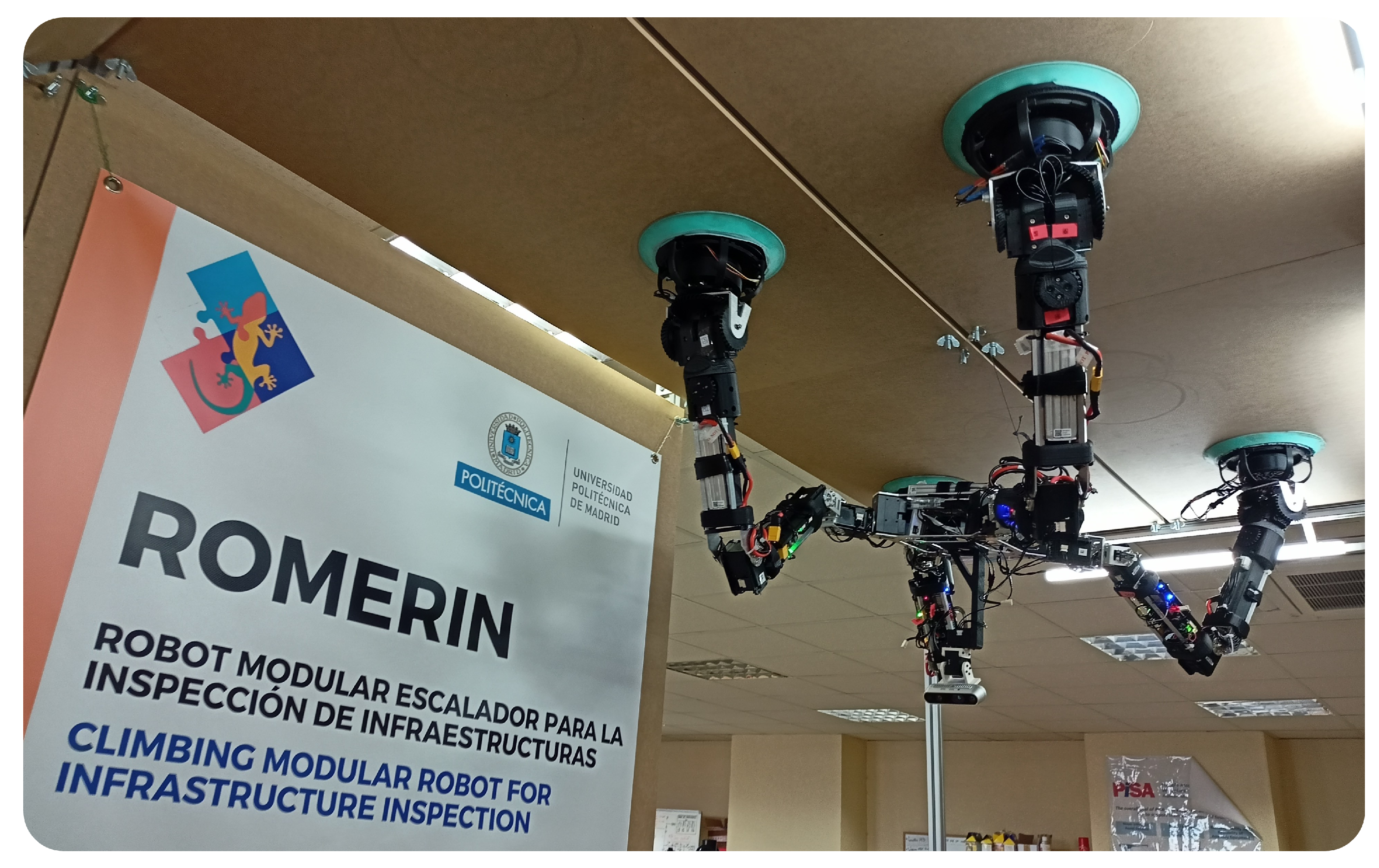
This article describes an efficient torque-based control algorithm for climbing robots with a variable number of legs. To do so, we introduce in first place the kinematic model of the ROMERIN robot [13] (Figure 1), a modular legged climbing robot for inspection and maintenance of large infrastructure, in which its components are coordinated and controlled by means of the MoCLORA architecture [14]. The robot is based on modular legs that have the ability to share energy in such a way that if the battery of one module stops working for any reason, the rest of the modules can share their energy, increasing the robustness of the robot [15].
We describe a torque-based control of multi-limbed hyperstatic systems. Most climbing legged robots have the peculiarity that they are hyperstatic structures when there is a physical adhesion between the gripping system and the surroundings. This fact makes it difficult and risky to control them exclusively with IKCs.
The main points and features of this article are summarized as follows:
  • Wrist actuators become passive whenever the adhesion system is attached to any surface. Thus, the complexity of the kinematic chain is reduced and, consequently, so is the complexity of the static model computation, which is implemented in a robot with a non-defined number of legs.
  • A low-weight computational method for computing the static model of a multi-limbed system is presented and, consequently, a gravity compensator is obtained.
  • Our static model solver method is compared with the most used one, which is based on the Lagrange equation method and the use of the robot Jacobian. The system is validated in both simulation and hardware experiments.
  • The results of the IKCs and the proposed torque-based control are compared using the same robot. The remarkable advantages of torque-based control are highlighted.
The article is organized as follows. In Section 2, we discuss the state-of-the-art legged and climbing robot and the types of controllers. The ROMERIN robot and its kinematic description are briefly presented in Section 3. In Section 4, we present a discussion of torque-based control for hyperstatic articulated systems, as well as the premises of the estimation of reaction forces. This section also includes a comparison between the most widely used approach and the one proposed in this article. In Section 5, the control techniques implemented under torque-based control are detailed, together with the position estimation of the robot. We end the article with results and conclusions in Section 6 and Section 7, respectively.

2. State of the Art

Legged robots can be classified according to their purpose (walking or climbing), leg kinematics, or number of legs. A common classification for leg kinematics distinguishes between articulated legs (with and without wheels), orthogonal legs, pantograph legs, or telescopic legs [4,16].
Articulated legs possess high maneuverability and flexibility compared to the other types of legs and are the most common leg structure found in the literature. Among the robots that use articulated legs, we find walking quadrupeds such as Spot [17], ANYmal [18], or StarlETH [19]. Nowadays these robots show great maneuverability and have advanced dynamic control thanks to sophisticated IDCs. Walking hexapods with articulated legs are very common. Some examples are LAURON [20], whose last version of the series (LAURON V) shows applicability over rough and hazardous terrains, RIMHO II [21], which includes sensors to detect and locate antipersonnel landmines, or OSCAR [22], which shows robustness against loss of legs. All these robots use IKCs to manage the position of the robot, and show no evidence of implementing torque-based controllers. It is also possible to find climbing quadrupeds with articulated legs, such as MRWALLSPECT-II [23], LEMUR [24], Magneto [25], or RVC [26], and climbing hexapods such as ROMHEX [27]. However, no evidence about torque-based controllers is found in the literature of these robots. Other articulated legged robots do not have a defined number of legs, such as the case of the walking robot Nimble Limbs [28], which uses an IKC, or the robot proposed in this article.
Robots that use orthogonal legs facilitate compensating the effect of gravity without large energy costs, but are less flexible than other leg types. Few recent studies on this type of leg structure are in the state of the art. As an example, in [29] the authors present a hexapod walking robot specifically designed for humanitarian demining applications, showing great energy efficiency and low power consumption. Regarding climbing robots using this leg configuration, one of the most relevant studies for quadrupeds is ROBOCLIMBER [30], which is a bulky quadruped climbing-and-walking machine capable of carrying heavy-duty drilling equipment for landslide consolidation and monitoring works. Ambler [31] and the wall climbing robot REST [32] are examples of cartesian coordinate hexapod robots. Torque-based controllers are not found in the description of these robots. In fact, this type of robot is not as dependent on static and dynamic calculation as robots with articulated legs, since they compensate the effect of gravity mainly thanks to their peculiar structure.
Pantograph legs have the advantage of decoupling horizontal and vertical motions. The legs are usually lighter due to the parallel mechanism they use, which allows the actuators to be located in the body. An example of a quadruped walking robot with this type of leg configuration is Oncilla [33], a bio-inspired low-weighted robot that shows agile and versatile locomotion, such as trotting on level ground, climbing and descending slopes, and turning. The adaptive suspension vehicle (ASV) [34] and MECANT I [35] are examples of hexapods that use pantograph legs controlled by IKCs. ASV, the largest hexapod in the world, was designed to carry cargo for industrial and military applications on rough, mountainous, icy, or muddy terrain. A relevant example of pantograph legs in climbing robots is SCALER [7], a quadrupedal robot that, in its climbing configuration, has 6DOF per leg. It demonstrates climbing walls, overhangs, ceilings, and trotting on the ground.
Telescopic legs, which have a compact structure, are primarily intended for bipeds [36,37], although there are other types of robots with this type of structure, such as quadrupeds [38] or hexapods [39].
Model-based control methods, such as IDCs, can be used to enable the fast, dexterous, and compliant motion of robots without sacrificing control accuracy. However, implementing such techniques on floating-base robots is not trivial because of underactuation, dynamically changing constraints from the environment, and potentially closed-loop kinematics. Most legged robots that use IDCs focus on floating-base systems by obtaining the Lagrange equations. In [40], the authors show how to analytically compute the inverse dynamics torques for model-based control of sufficiently constrained floating base rigid body systems, such as humanoid robots with one or two feet in contact with the environment. Similarly, in [41] the authors present an inverse dynamics controller for legged robots that use torque redundancy to create an optimal distribution of contact constraints. In [12], the authors present the dynamic model of a 5DOF wall-climbing robot, which can be considered an open-loop chain, since it has only two grippers and alternates their adhesion.

3. ROMERIN Modular Climbing Robot

3.1. Brief Description of the ROMERIN Leg Module

In this article, we work directly with the ROMERIN robot (Figure 1), whose legs modules are presented in [15]. These modules have been slightly modified, so that the leg modules used in this article are made up of DYNAMIXEL servomotors grouped into three groups, shoulder (2-DOF), elbow (1-DOF), and wrist (3-DOF). The servomotor models are, in this case, MX-64T ( q 1 ), XH540-W270-T ( q 2 q 3 ), and XL430-W250-T ( q 4 q 6 ). The axes of the last three joints (wrist) are arranged concurrently, with the last two axes in a differential configuration. As a result of that, similarly to what happens in most industrial robots, the last three axes intersect at the same point (called the wrist point) in such a way that whenever the gripping system is grabbed to a surface, the wrist point stays static.
Each module has its own battery and has the ability to share energy with other modules in case of battery failure. The control of the servomotors is carried out by an ESP32 microcontroller (MCU), located on an electronic board, according to the commands given by a central computer where coordination of the legs is performed [14]. The MCU is also able to control the end-effector tool, a suction cup with a turbine that allows a vacuum to be generated. This tool has a pressure and temperature sensor as well as three laser distance transducers that are used to facilitate the alignment of the suction cup with a surface. With feedback from the pressure sensor, it is immediately possible to determine the gripping force achieved by the suction cup, whose design, efficiency, and performance are described in more detail in [42]. The weight and length of the entire module is 1.94 kg and 0.86 m, respectively.
A set of leg modules makes up a modular legged-and-climbing robot able to walk and climb on different materials and in different orientations. In the next subsection, an analysis of the kinematic model of each leg, as well as its simplification for future sections, is included, in order to obtain a torque-based control for the modular legged and climbing robot.

3.2. Kinematic Model of ROMERIN

In general, a modular robot of N identical modules is assumed, where module i [ 1 , , N ] has J joints and K links indicated as j [ 1 , , J ] and k [ 1 , , K ] . The mass of the link k of the module i is denoted as m i k , while m i is the total weight of the module i, and L its maximum length. A common situation is one in which all the modules of the robot are correctly adhered to the environment by means of a grip system, such as suction cups or magnets, having a free ball joint located in the WP (wrist point) that allows the free orientation of the end effector against the surface of the environment. The body is rigid and therefore has constant dimensions and a mass of m B , while the angles of the joints are denoted as q i j . The mass of the entire ROMERIN robot is denoted as M. The reference systems (Figure 2) are located at the origin of the body Σ B (located in the center of mass, COM, by own decision), in the first joint of each module Σ i , in the WP Σ i w , at the contact points Σ i S , and in the COM of each link Σ i k , of each module Σ i , c g and of the whole robot Σ c g . Due to the interaction of the robot with the environment and the detachment of the wrist actuator, reaction forces F i , appear at the wrist point Σ i w . The homogeneous transformation matrix between the reference systems Σ B and Σ i is denoted as T i B . The transformation from Σ B to Σ i j is denoted as T i j B . Lastly, Σ C represents the reference frame of the camera, where the embedded IMU is located.
The kinematic model of each module is shown in Figure 3, whose main dimensions and masses are denoted in Table 1. The Denavit–Hartenberg (DH) parameters that define the kinematic model are indicated in Table 2.
To reduce the problems of hyperstaticity, to simplify the kinematic chain, and to be able to compute the reaction forces in the WP, the wrist is disabled when the suction cup is attached to a surface; that is, the last three joints are detached from the power, keeping the feedback from them. To reduce computation complexity, the system can be reduced as shown in Figure 4, with the premises:
α = a t a n ( L 3 L 2 ) = 0.09561
L c = L 2 2 + L 3 2 = 0.22095
β = a t a n ( L 5 L 4 ) = 0.08004
L d = L 4 2 + L 5 2 = 0.28081
In this case, the feedback position of the motors should be transformed, as well as the commanded position for each motor. That is, the second joint receives an increment of α , while the third joint receives an increment of α + β (positive or negative according to the direction).
For the simplified case, the forward kinematic model of each leg is computed as indicated in Equation (5), whose differential is obtained in Equation (6).
x w y w z w = L 1 · c 1 + L c · c 1 · c 2 + L d · c 1 · c 3 2 L 1 · s 1 + L c · s 1 · c 2 + L d · s 1 · c 3 2 L c · s 2 L d · s 3 2
x ˙ w y ˙ w z ˙ w = s 1 · L 1 + L c · c 2 + L d · c 3 2 L c · c 1 · s 2 + L d · c 1 · s 3 2 L d · c 1 · s 3 2 c 1 · L 1 + L c · c 2 + L d · c 3 2 L c · s 1 · s 2 + L d · s 1 · s 3 2 L d · s 1 · s 3 2 0 L c · c 2 + L d · c 3 2 L d · c 3 2 J ( q ) · q 1 ˙ q 2 ˙ q 3 ˙
In this case, inverse kinematics is obtained by:
q 1 = a t a n 2 ( y w , x w )
q 3 = arccos x w c 1 L 1 2 + z w 2 L c 2 L d 2 2 · L c · L d
q 2 = a t a n 2 z w , x w c 1 L 1 + a t a n 2 L d · s 2 , L c + L d · c 2
Although the calculation of q 3 should be considered in two ways, positive and negative, only positive values are considered to avoid that the elbow goes under the body.

4. Torque-Based Control of Hyper-Static Multi-Limbed Systems

As denoted previously, control of multi-body robotic systems can be controlled by two types of controller, IKCs and IDCs. Our control system makes use of both, trying to take advantage of each approach. This responds to two different situations for the leg:
  • When the leg is attached to the environment, the interaction between both is reflected in the appearance of reaction forces. In this case, the module should be controlled by an IDC to avoid an overload of the actuators due to the closing of the kinematic chain.
  • When the leg is detached and free, no reaction forces appear in the leg, and therefore it can be controlled with an IKC or by means of an IDC.
One of the problems studied for multi-legged robots is how to determine the best sequence to lift and place the feet [43]. Non-climbing multi-legged robot locomotion can be classified into dynamic locomotion (running and hopping), and static locomotion as walking, where the body is constantly stable. For them, the vertical projection of the center of gravity of the robot has to be within the supporting polygon that links the positions of all supporting feet.
For bio-inspired climbing robots, the dynamic gait is a faster and more difficult style, similar to other non-climbing legged robots. Several models describe dynamic gait to improve robot speed. The spring-mass model consisting of a massless spring attached to a point mass describe the interdependency of mechanical parameters that characterize the running and jumping of humans as a function of speed [44]. Robots with dynamic gaits, such as [45] or [46], have been proven to be feasible with a pendulum mechanism or springs. Furthermore, the adhesion system has to work practically instantaneously to guarantee the dynamic gait. They also face the problem that their applications are so far limited to climbing on a plane.
For a system such as the one proposed in this article, dynamic gait is discarded because of the attaching/detaching process of the suction cup, and because of safety reasons (related as well to the adhesion system). In fact, for the first of the situations proposed at the beginning of this section, each module of the robot has very low speed and acceleration. Thus, the inertial and centrifugal components of the dynamic model can be neglected with respect to the gravitational component. This problem simplification concludes in the static model of the system (Equation (11)), where only the forces and torques produced by the action of gravity and the reaction forces appear. The result of the equation is related to the torques that each joint has to apply to compensate for body weight.
τ = M ( q ) · q ¨ 0 + C ( q , q ˙ ) · q ¨ 0 + g ( q ) + J ( q ) T · F e x t
τ = g ( q ) + J ( q ) T · F e x t
This robot has N · J controllable DOFs, of which N · 3 are forced to be passive when the leg module is attached (wrist), while only six DOFs related to body position and orientation can be controlled ( R 3 SO(3)). The system is hyperstatic when, while the gripper system is attached to the environment, there are more DOFs to act than DOFs to control. As this difference increases, the system becomes more complex and more inaccuracies are penalized in the estimation of the torques to be applied. The passivity of the wrist is made by deactivating the power of the actuators, and it reduces hyperstaticity and allows for computing the force distribution problem (FDP). Many legged robots use force/torque sensors to skip FDP and reduce software complexity, while increasing platform costs [7].

4.1. Force Distribution Problem (FDP)

The force distribution problem is one of the challenges for legged robots. According to the characteristics of multi-chain systems of legged robots, it is explicitly remarked that the chains located in the support phase are tightly attached to each other [4]. This fact has been highlighted in this dissertation as the hyperstatic problem.
Generally, during the stance phase, the reaction forces that appear in the robot have to meet physical constraints to be valid:
  • For a walking legged robot located in the z-plane (opposite to the gravity vector), the normal contact forces of the support feet are positive:
    F i , z 0
    This means that if the legged robot is walking on a slope (moving on x-direction), positive tangential forces are strictly required during the stance phase:
    F i , x 0
    On the other hand, for climbing legged robots, the normal contact forces of the support can be as negative as desired, as long as it is ensured that the torque of the actuators does not exceed the permissible limits (point 4), and the suction cup is not at risk of detaching from the surface.
  • The total normal force of the stance phase is equal to the force produced by the weight of the legged robot. That is, the sum of the reaction forces compensates the gravitation component, and the sum of the momentum is zero:
    Σ F i + M · g = 0
    M i = 0
    When force/torque sensors are used on the feet, it is possible to observe that the values differ slightly due to motion, assumptions, and inaccuracies. When estimating forces by solving the FDP, the values may differ slightly due to set thresholds for the convergence of numerical methods. Similarly, for climbing robots, there should also be a moment equilibrium.
  • For legged robots, the support feet must not slip:
    F i , x 2 + F i , y 2 μ F i , z
    where F i , x and F i , y are the foot forces of leg i of the support phase in the x and y directions, respectively, and μ is considered the relevant friction coefficient of the ground. For climbing robots, the normal force must be lower than a limit value, which is generally denoted as the grip force F s c :
    F i , z < F s c
  • Finally, the torques in each actuator have to be lower than their torque limits:
    τ i , m a x J i T · F i i τ i , m a x
    where τ i , m a x R J × 1 is the maximum articulated torque vector of the leg i; J i T R J × 3 is the Jacobian of the leg i; and F i i is the reaction forces related to Σ i .
The solution of FDP for legged robots is a complex mathematical programming problem [4]. The main solving methodologies are as follows:
  • Linear-Programming (LP) Method. It is known as the most common programming algorithm for optimizing FDP [47], but many flaws have been detected during its implementation, such as computational cost or discontinuity.
  • Compact-Dual Linear-Programming (CDLP) Method. It results in a smaller size problem compared to the LP method by using compact-dual linear programming, but it is unable to completely overcome discontinuity issues [48].
  • Quadratic-Programming (QP) Method. This method presents the advantage that its computing time does not depend on the initial hypotheses. In addition, it is able to solve the discontinuity problem [49,50].
  • Analytical Method. This method is implemented mainly for walking robots. It consists of balancing the forces of the support feet in order to prevent legs from slipping.
In this article, we implement the alternative presented in [
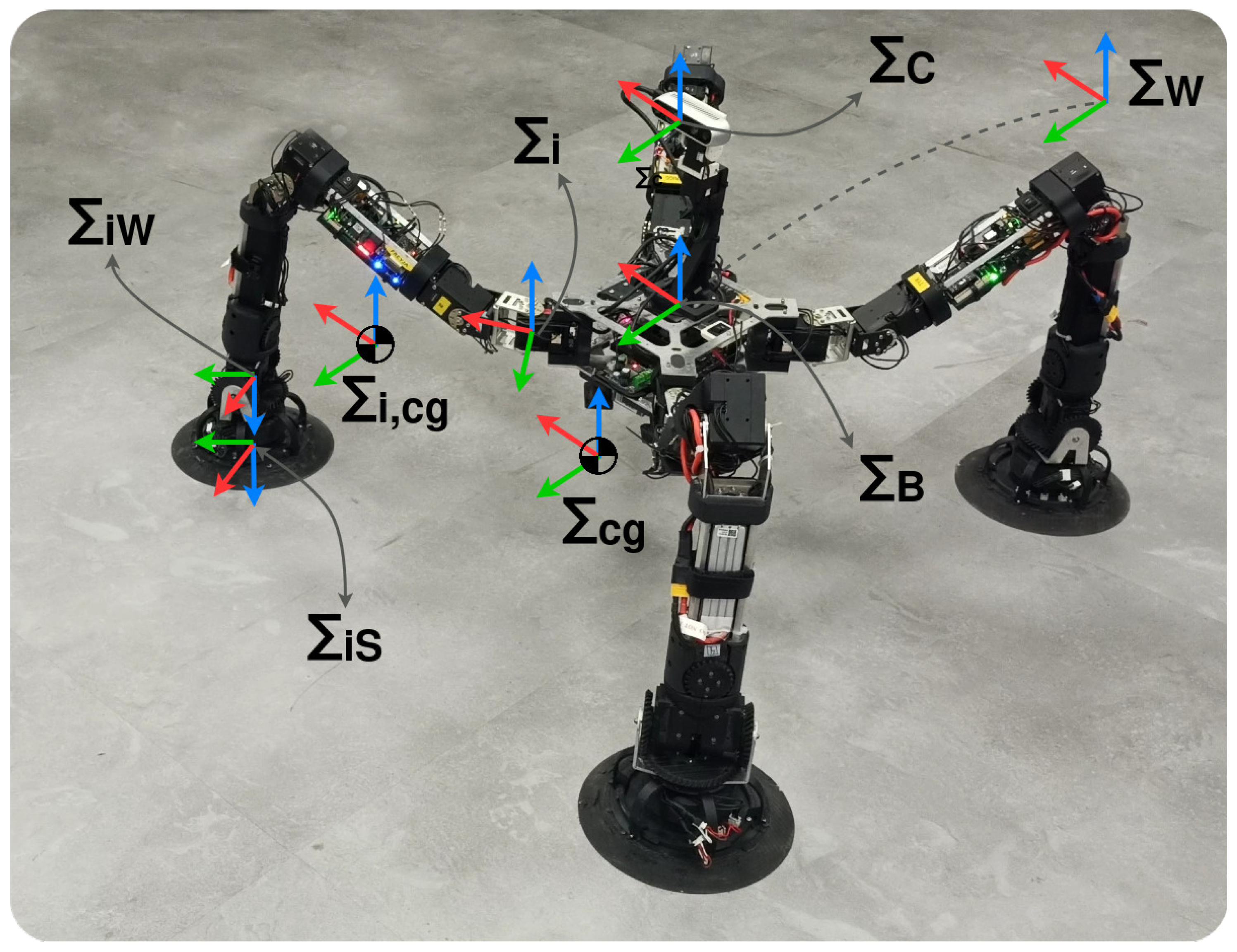
51], where the problem of a hyperstatic system is attacked. The reaction forces are referred to the gravity center. Thus, first of all, one must calculate the gravity center of the robotic robot. A model-based computation can be applied since the position of each joint is well known thanks to the embedded encoders, as well as the mass and the dimensions of the links and body.
To do so, each leg calculates its own gravity center with respect to its own reference frame. A crucial part is that the mass of the gripping system is ignored when the suction cup is attached to a surface because it could be considered part of the environment. For the following equations, Σ i i , c g represents the position of the gravity center of the leg i referred to the reference frame 
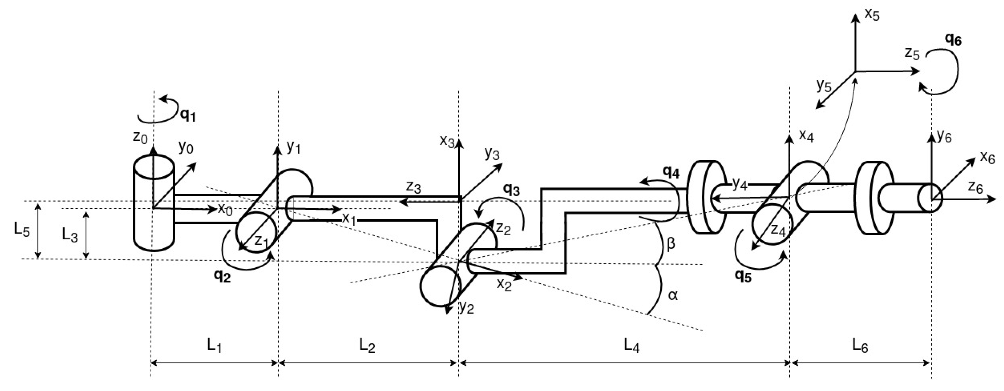
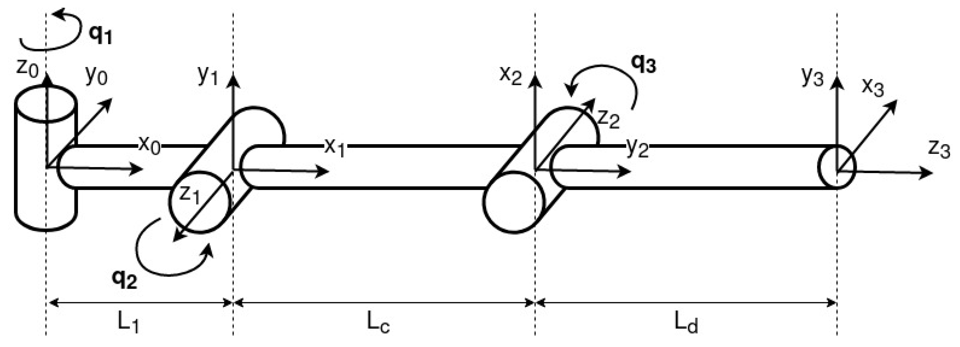
A. Then, for each non-supporting leg (swing phase), the kinematic model presented in Table 2 and Figure 3 is used, and the gravity center of the leg i is calculated as:
Σ i i , c g = 1 m i · k = 1 K x i k i · m i k
On the other hand, for each supporting leg (stance phase), the gravity center of leg i is computed (with Z = K 3 ) as:
Σ i i , c g = 1 m i 1 + m i 2 + m i 3 · k = 1 Z x i k i · m i k
For both cases, supporting and non-supporting legs, the position of the leg gravity center is transformed to Σ B as:
Σ B i , c g = P i B · Σ i i , c g
where P i B denotes the position transform from Σ B to Σ i , and therefore, the gravity center of the whole system (referred to Σ B ) is given by:
Σ B c g = 1 M i = 1 N m i · Σ B i , c g
where M represents the robot mass that is considered for the computation of the reaction forces, m i = m i for non-supporting legs, and m i = m i 1 + m i 2 + m i 3 for supporting legs. Being N s and N n , the number of supporting and non-supporting legs, respectively, the value of M is given by:
M = m B + N s · m i 1 + m i 2 + m i 3 + N n · m i
The position of the wrist points (where the reaction force appears) and the total center of mass of the robot are required to compute the reaction forces with the implemented estimator. To do so, Equation (24) denotes the transformation between the center of gravity and the Wrist Point (WP) pose as:
T w c g = T c g B 1 · T i B · T w i
where T w i can be obtained with the forward kinematics given by Equation (5), and T c g B is given by Equation (23). For simplicity, Σ c g is located with the same orientation as Σ B .
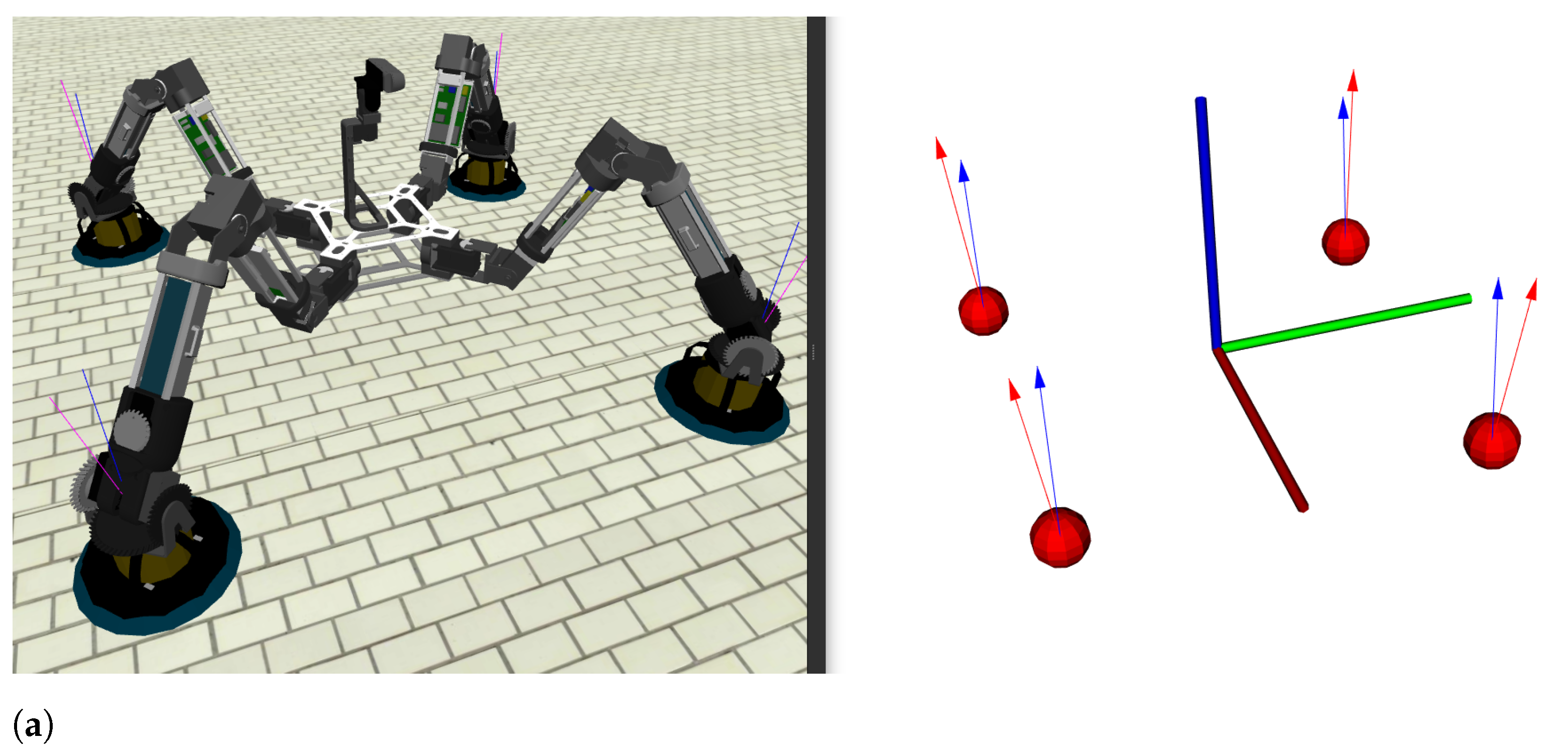
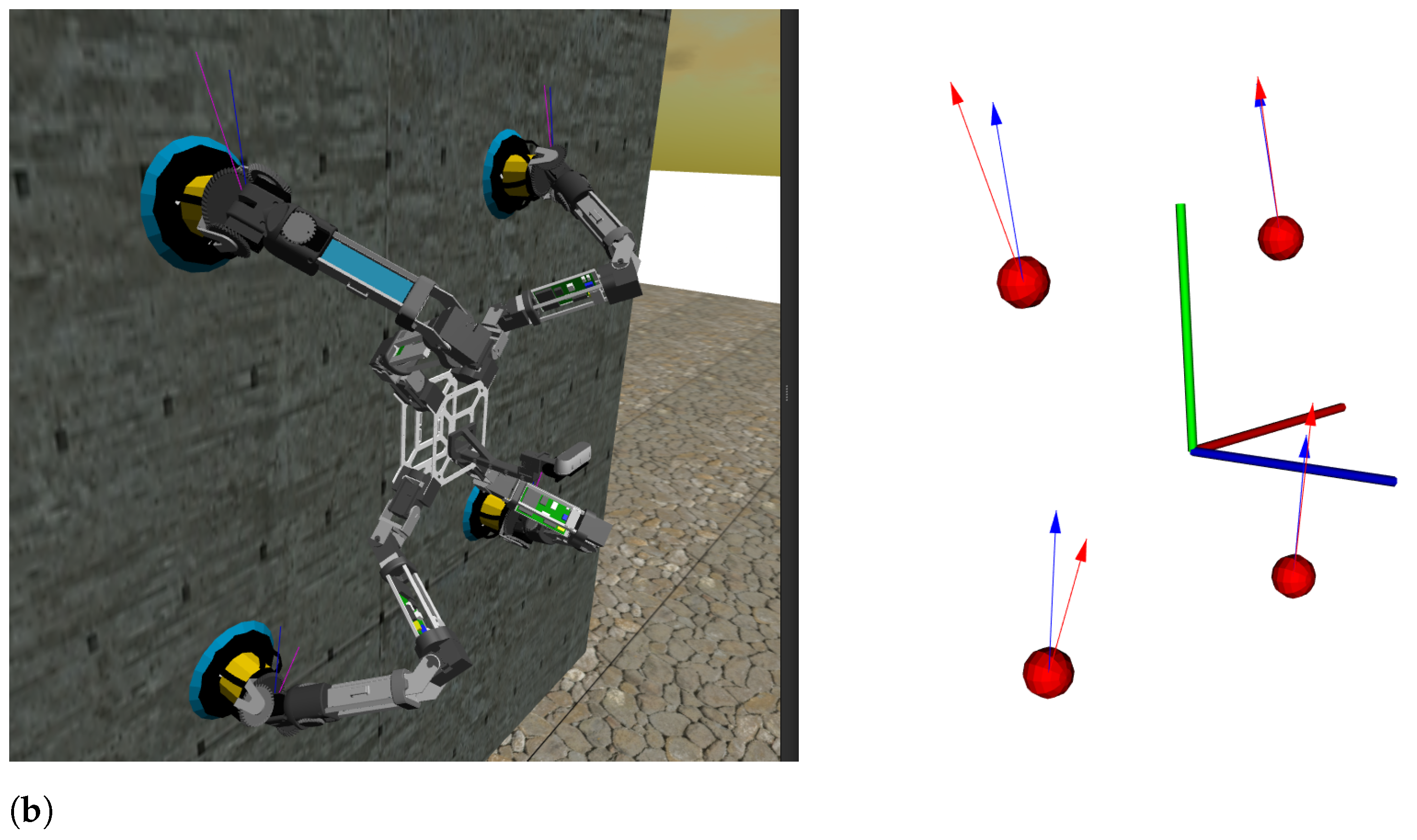
Once the position of the WPs and the direction of the gravity vector are known thanks to an integrated IMU in the body, the reaction forces can be computed as presented in [51]. As an example, in Figure 5 two examples of the reaction forces that appear in the WPs when the robot is in a static central position are illustrated.

4.2. Classical Method

In the world of static forces the transpose of the robot Jacobian relates the forces exerted by the end-effector to the forces exerted by each joint. Thus, according to the classical method, Equation (25) indicates how to calculate the torques required whenever an external force is applied to the end effector.
τ e x t = J ( q ) T · F e x t
Regarding the gravitational component, it can be obtained by means of analytical ways: Euler–Lagrange [52], recursive Lagrange [53], recursive Newton–Euler [54], Kane’s equations [55], the D’Alembert principle [56], and some alternate algorithms that are based on velocity constraint matrices [57] or a divide-and-conquer approach [58].

4.3. Implemented Method

In order to solve Equation (11), we propose a method to compute the torque that each actuator has to apply to compensate gravitation forces without the use of the Jacobian matrix for the forces exerted by the end-effector and without the use of other analytical calculations for the gravitational components.
In this method, the Newton–Euler method is used. Basically, the Newton–Euler equations describe the combined translations and rotational dynamics of a rigid body. They are used as the basis for more complicated "multi-body" formulations (screw theory) that describe the dynamics of systems of rigid bodies connected by joints and other constraints. Multi-body problems can be solved by a variety of numerical algorithms [59]; however, for our specific case, we have formulated Algorithm 1. It is presented from a modular point of view, where each module computes the torques required to compensate gravitational forces.
Algorithm 1 Gravity torque compensator of module i
Outputs:  τ [ J ]
1:for  j Σ i j  do
2:    for  k Σ i k  do
3:        if  j > i  then
4:           Skip ▹ Only child links
5:         r d i s t a n c e V e c t o r ( Σ i j , Σ i k )
6:         F m k · g
7:         T r × F ▹ Weight torques
8:         T t o t a l = T t o t a l T
9: 
10:     r d i s t a n c e V e c t o r ( Σ i j , Σ i w )
11:     T r × F i ▹ Torques related to the external forces applied at WP
12:     T t o t a l = T t o t a l T
13: 
14:     τ [ i ] = u q · T t o t a l ▹ Project to j joint axis
The torques required to compensate the gravity forces are calculated for each joint. Equation (26) calculates the momentum produced on an object based on the amount of force applied, F to the object at a distance, r , from the pivot point from where the force is applied to the pivot point of the object. In the formula, u q represents the unitary vector that projects the moment on the joint axis.
τ = u q · r × F
In a similar way to the resolution of bending moment diagrams, a hyperstatic system can be approached by analyzing the forces that appear on it at certain points of interest (in this case, at the joints of the robot). By making a section at each of the joints, an analysis of the forces remaining on one of the sides is performed. The simplest way is to apply the forces appearing in the module itself, i.e., the weights of the links farthest from the body and the reaction force appearing in the given module.

4.4. Comparison of Methods

The methods presented in Section 4.2 and Section 4.3, respectively, give the same results under the same conditions. The first method has been widely used for legged robots, and it is one of the unique methods found in the literature. A great example is [60], where the authors use the Jacobian transpose to compute the torques required by external forces, which are computed thanks to the combination of the QP method with the reduction in the problem size proposed in [61] to solve the FDP.
Table 3 indicates the computation time for each method for one leg (including the standard deviation) and for a modular robot of four and six legs. Although the growth of the computation time is linear for both cases, it is possible to observe that as the number of legs increases, the computation time for the first method increases considerably. It is particularly important for a multi-legged system where the logic runs on a single computer and where the control rate and computational cost are critical. This importance increases for systems such as ROMERIN, where the number of legs can be considerably increased to adapt to specific real-time applications. In addition, it is especially important in sampling-based algorithms for motion planning, where the computation is performed many times.
As denoted in the table, the average computational cost of the proposed method is half that of the classical method. This is due to the use of the Jacobian matrix, which increases the computation requirements. To point out the importance of reducing computational time, in the case of using a sampling-based algorithm for motion planning in an hexapod robot, the proposed method in this article saves 0.41 s of computation with 1000 samples.
Additionally, the implementation of the proposed method can be very simple by using packages tf or tf2 from ROS and ROS2, respectively. These tools could help the developer create a torque-based control in a simple and fast way, even without developing a detailed kinematic model.

5. Impedance Control of Leg Modules

There are two main alternatives to control the position of the robot while sending torque commands [62]. The first case is the proportional control plus velocity feedback, whereas the second case is the PD control. Both cases represent closed-loop controllers, where the proportional and derivative constants help the modules push the body of the robot.
The proportional control plus velocity feedback with gravity compensation is the simplest closed-loop controller that may be used to control robot manipulators. The conceptual application of this control strategy is common in angular position control of DC motors. In this application, the controller is also known as a proportional control with tachometric feedback. The equation of proportional control plus velocity feedback is given by Equation (27), where K p and K d R n × n are symmetric positive definite matrices that refer to the position gain and the velocity gain (or derivative), respectively, and τ g refers to Equation (11).
τ = τ g + K p · q d q K d · q ˙
On the other hand, the proportional Derivative (PD) control with gravity compensation is an immediate extension of proportional control plus velocity feedback. As its name suggests, the control law is not only composed of a proportional term of the position error as in the case of proportional control, but also of another term which is proportional to the derivative of the position, i.e., to its velocity error:
τ = τ g + K p · q d q + K d · q ˙ d q ˙
Proportional control plus velocity feedback may be understood as a PD control where the desired velocity is zero to guarantee stability and reduce rude movements.
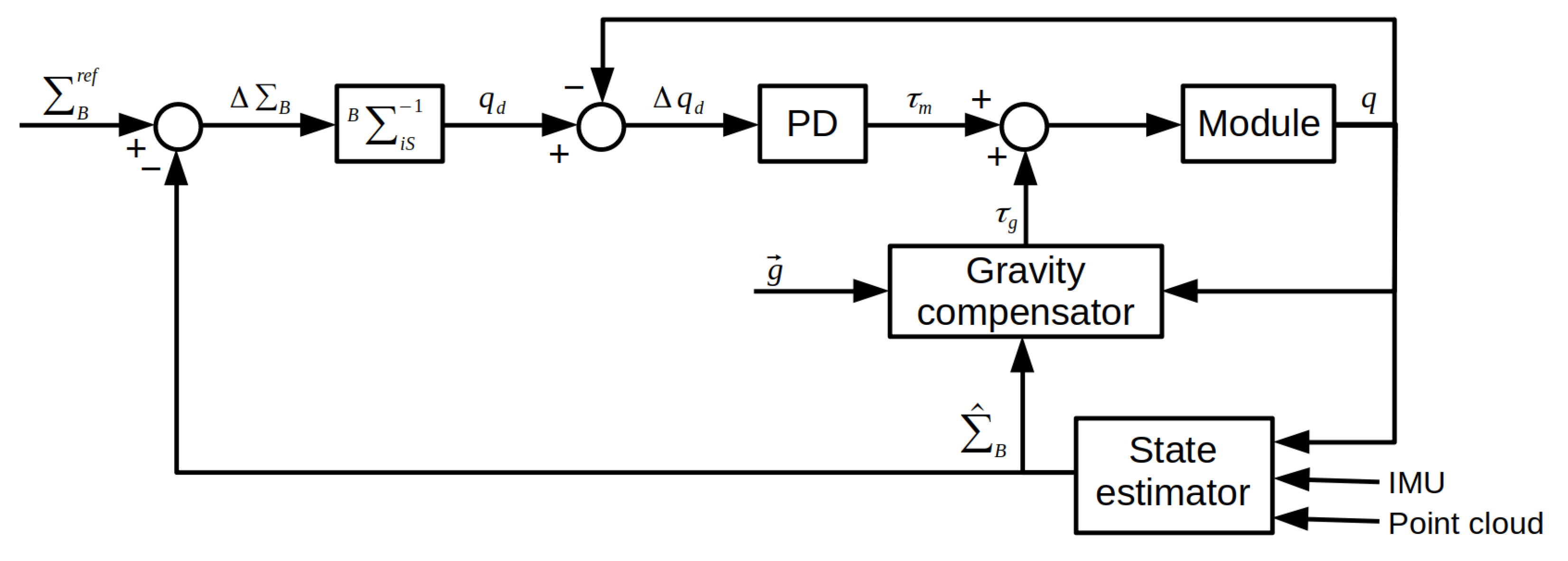
Figure 6 shows the control diagram that is integrated in each module, which can be denoted as an impedance control. A body position is commanded Σ B r e f and compared with the estimated body position Σ ^ B . The transformation B Σ i w 1 is applied to obtain the desired joint position q via B T i and the inverse kinematics. A PD controller is applied to obtain the torque based on the joint position error. On the other hand, based on the position estimation and the gravity compensator proposed in this section, another torque component is generated. The sum of both torques is applied to the joints.

5.1. State Estimator

Body position estimation is implemented from [63]. It takes the robot and IMU odometry as input and fuses them with an Extended Kalman Filter (EKF). Later, it uses points clouds from the mounted RGBd camera to perform a graph-SLAM approach. Body position odometry is obtained through the FK of the supporting legs. Because the initial state of the robot is known, the body position is straightforwardly computed as:
Σ ^ B i = B Σ i · i Σ i S , t = 0 · i Σ i S , t = k 1 · B Σ i 1
where Σ ^ B i is the estimation of the position of the body frame by the module i, B Σ i the transformation from the body frame to the first joint frame of the module i, i Σ i S , t = 0 its FK in the initial state, and i Σ i S , t = k its FK at time k. Since there is the same number of valid solutions as legs, currently the robot odometry is implemented as the average of them as:
Σ ^ B = 1 N i = 1 N Σ ^ B i
On the other hand, the mean robot orientation odometry can be computed as:
Q = [ a 1 q 1 , a 2 q 2 , . . . , a N q N ]
where a i is the weight of the i t h quaternion ( q i ) averaged, included as a column vector. In this case, given the modularity of the robot, a i is evenly distributed. Q is therefore a 4 × N matrix.
The normalized eigenvector corresponding to the largest eigenvalue of Q Q T is the weighted average. Since Q Q T is self-adjointed and at least positive, semi-definite, fast, and robust methods of solving that eigen problem are available. Furthermore, this is scalable. Computing the matrix–matrix product is the only step that grows with the number of elements that are averaged.

5.2. Body Trajectory Tracking Control

Following the objective of biomimetics, in this section we describe the body trajectory tracking control without dynamic compensation used in the ROMERIN robot. In the animal world, the body position is usually not controlled directly. On the contrary, animals “establish” their body velocity, and the legs are those that accompany the movement.
Unlike path-following, which focuses on following a predefined path without time constraints, trajectory tracking does not guarantee that the path is faithfully followed. Instead, it involves time as a constraint by correcting the position error. Thus, for the ROMERIN robot, a body velocity control without dynamic compensation is described as:
x ˙ = x ˙ d + K B · x ˜
where K B denotes the constant that attempts to correct the position error.

6. Experiments

ROMERIN capabilities and performance were evaluated and demonstrated in discrete and continuous environments and ground tests listed in Table 4. ROMERIN can climb vertical walls while walking on the ground and the ceiling (Video available at https://youtu.be/nTHPNJAwBs4, accessed on 18 July 2023).

6.1. Torque-Based Control Experiment

ROMERIN was operated using a predefined manual circular trajectory to verify the combination of the FDP solver and impedance control. IMU data are given by the embedded RealSense D435i IMU and transformed to Σ B as:
g B x g B y g B z = R B C · g C x g C y g C z
where R B C denotes the rotation matrix from Σ B to Σ C . Figure 7 shows the behavior of a PD control with gravity compensation, where the constants that are given experimentally are:
K p = 40 60 25 ; K d = 8 10 5 ; K B = 0.1 0.1 0.1 0.15 0.15 0.15
and the maximum allowed torque has been set to 65% of the actuator stall torque to avoid overloads. The position and the resultant torques are shown in Figure 8, while the cartesian position of the same leg Σ i S related to Σ i is illustrated in Figure 9. As observed, the leg follows the received commands, where the maximum error is found in the ’Z’ axis, which corresponds to the gravity component. The mean body position error has been reduced from 0.2 ± 0.05 rad and 6.0 ± 1.5 cm of the ROMERIN IKC [14], to 0.1 ± 0.02 rad and 3.0 ± 0.6 cm with the proposed torque-based controller of this article.

6.2. Gravity Compensation

The same predefined manual circular trajectory to verify the combination of FDP solver and impedance control has been tested in different situations, such as on the ground, wall, and ceiling. In this case, the PD component has been removed from time to time, keeping gravity compensation only. To verify the performance of gravity compensation, the ROMERIN digital twin [14], which can be configured to only accept torque commands, has been used. In this way, thanks to its reliability, it is possible to verify the experiments from a theoretical point of view. It has been demonstrated that when the PD component is removed, the robot stays still in different situations. Figure 10 shows the example where the robot is in the ceiling. As observed, the joints follow the commands faithfully and remain constant when the PD component is removed (blue boxes), keeping the gravity compensation only. For this experiment, constant values of Equation (34) are set.

6.3. ROMERIN Gait

ROMERIN gait has been tested in the ground, inclined walls, vertical walls, and ceilings. As an example, Figure 11 shows screenshots of the behavior of a quadruped configuration over an inclined wall of 45 . Similarly, Figure 12 shows the behavior of the ROMERIN hexapod configuration on a vertical wall.

7. Conclusions

In this article, the Newton–Euler formulation was used to develop a novel, platform-generic, low-weight, fast-implemented, and agile method of gravity compensation. By describing the combined translations and rotational dynamics of a rigid body, the basis for more complicated “multibody” formulations that describe the dynamics of systems of rigid bodies connected by joints and other constraints has been presented. To do so, we have presented the algorithm over the ROMERIN robot, which is a modular legged-and-climbing robot with an undefined morphology.
We first introduced the detachment of the adhesion system when performing the static computation of forces, reducing the complexity of the kinematic chain. In addition, we made use of a reliable reaction force estimator and tested it under multiple scenarios. The estimator takes advantage of the passivity of the wrist actuators to balance the momentums at the wrist points. In order to solve the static problem, which is a reduction in the dynamic model of the robot, we introduced the ROMERIN legs’ kinematics, which are required to compute the center of gravity of the entire robot, the gravity compensation by classical methods, and the estimation of the robot state. Consequently, we presented the low-weight computational method to compute the static model of a multi-limbed system, and we compared the method with the classical one, validating it with both hardware and simulated robots.
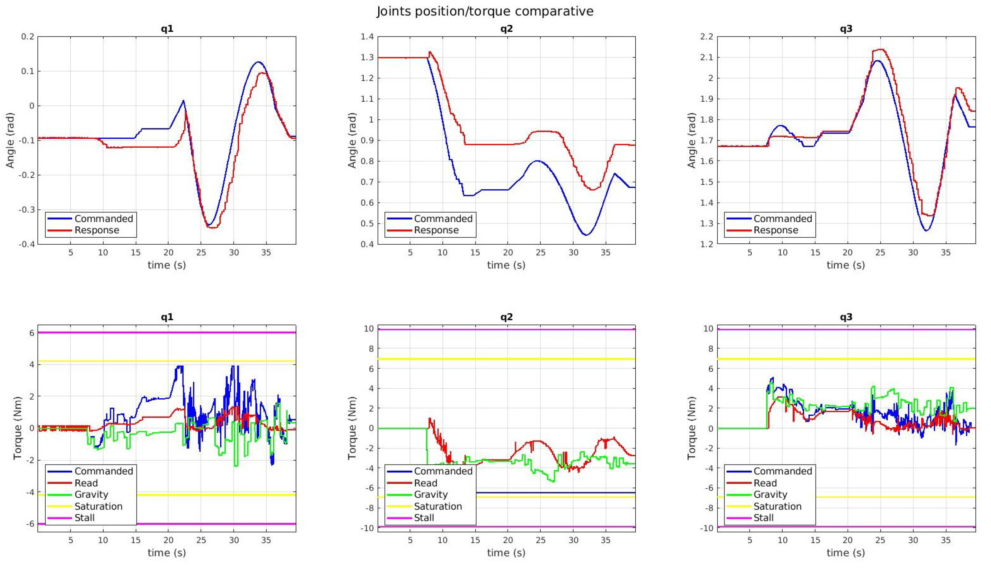
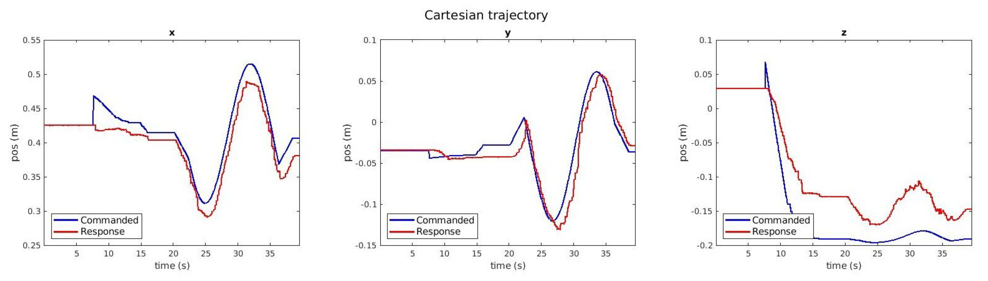
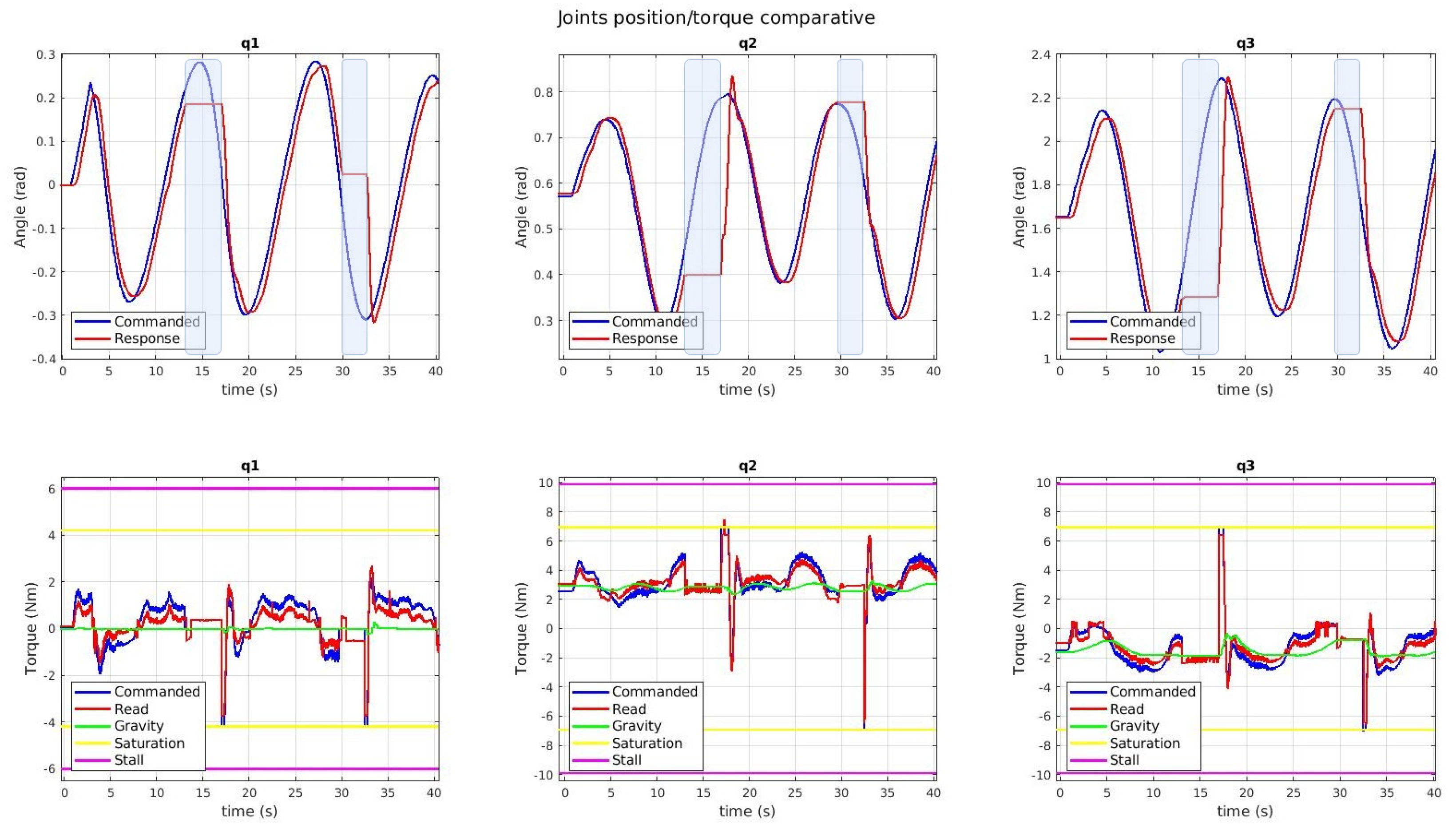
Comparing the results by using IKCs and the proposed torque-based controller with the same robot, it is possible to conclude that the mean angular and linear error is reduced considerably, as well as the power requirements of the actuators, which is a critical part in articulated multi-limbed robots.

Author Contributions

Conceptualization, C.P., M.H. and E.G.; methodology, C.P., M.H. and E.G.; software, C.P.; validation, C.P.; formal analysis, C.P.; investigation, C.P.; resources, C.P.; data curation, C.P.; writing—original draft preparation, C.P.; writing—review and editing, M.H. and E.G.; visualization, C.P.; supervision, M.H. and E.G.; project administration, M.H., E.G. and A.B.; funding acquisition, M.H., E.G. and A.B. All authors have read and agreed to the published version of the manuscript.

Funding

The research leading to these results has received funding from RoboCity2030-DIH-CM, Madrid Robotics Digital Innovation Hub, S2018/NMT-4331, funded by “Programas de Actividades I+D en la Comunidad de Madrid” and co-financed by Structural Funds of the EU. The project in which this research is being developed was initially funded by the Spanish National Plan for Scientific and Technical Research and Innovation, DPI2017-85738-R.

Institutional Review Board Statement

Not applicable.

Informed Consent Statement

Not applicable.

Data Availability Statement

Not applicable.

Acknowledgments

The authors would like to thank all the students that have worked on the ROMERIN project. In particular, it is worth mentioning Javier Valero for the manufacturing of the modules, Alejandro Figueroa for the electronic redesign, Mateo Agustoni for the suction cup manufacturing, and Fernando de las Heras for the environment design.

Conflicts of Interest

The authors declare no conflict of interest.

Abbreviations

The following abbreviations are used in this manuscript:
IKCInverse kinematic controller
IKDInverse dynamic controller
MoCLORAModular Climbing-and-Legged Robotic Organism Architecture
WPWrist point
COMCenter of mass
DHDenavit–Hartenberg
DOFDegrees of freedom
FDPForce distribution problem
EKFExtended Kalman Filter

References

  1. Katz, D.; Kenney, J.; Brock, O. How Can Robots Succeed in Uunstructured Environments. In Workshop on Robot Manipulation: Intelligence in Human Environments at Robotics: Science and Systems; Citeseer 2008. Available online: https://citeseerx.ist.psu.edu/doc_view/pid/892f1e4f5b26d0ab44a11de385d95f152d1e6bd0 (accessed on 16 July 2023).
  2. Prados Sesmero, C.; Buonocore, L.R.; Di Castro, M. Omnidirectional Robotic Platform for Surveillance of Particle Accelerator Environments with Limited Space Areas. Appl. Sci. 2021, 11, 6631. [Google Scholar] [CrossRef]
  3. Picardi, G.; Astolfi, A.; Chatzievangelou, D.; Aguzzi, J.; Calisti, M. Underwater legged robotics: Review and perspectives. Bioinspir. Biomim. 2023, 18, 031001. [Google Scholar] [CrossRef] [PubMed]
  4. Zhuang, H.; Gao, H.; Deng, Z.; Ding, L.; Liu, Z. A review of heavy-duty legged robots. Sci. China Technol. Sci. 2013, 57, 298–314. [Google Scholar] [CrossRef]
  5. Roth, Z. Machines that walk: The adaptive suspension vehicle. Mech. Mach. Theory 1990, 25, 587. [Google Scholar] [CrossRef]
  6. Li, J.; Gao, H.; Wan, Y.; Humphreys, J.; Peers, C.; Yu, H.; Zhou, C. Whole-Body Control for a Torque-Controlled Legged Mobile Manipulator. Actuators 2022, 11, 304. [Google Scholar] [CrossRef]
  7. Tanaka, Y.; Shirai, Y.; Lin, X.; Schperberg, A.; Kato, H.; Swerdlow, A.; Kumagai, N.; Hong, D. SCALER: A Tough Versatile Quadruped Free-Climber Robot. In Proceedings of the 2022 IEEE/RSJ International Conference on Intelligent Robots and Systems (IROS), Kyoto, Japan, 23–27 October 2022. [Google Scholar] [CrossRef]
  8. Qiaoling, D.; Yan, L.; Sinan, L. Design of a micro pole-climbing robot. Int. J. Adv. Robot. Syst. 2019, 16, 172988141985281. [Google Scholar] [CrossRef]
  9. Kim, D.; Di Carlo, J.; Katz, B.; Bledt, G.; Kim, S. Highly dynamic quadruped locomotion via whole-body impulse control and model predictive control. arXiv 2019, arXiv:1909.06586. [Google Scholar]
  10. Bellicoso, C.D.; Gehring, C.; Hwangbo, J.; Fankhauser, P.; Hutter, M. Perception-less terrain adaptation through whole body control and hierarchical optimization. In Proceedings of the 2016 IEEE-RAS 16th International Conference on Humanoid Robots (Humanoids), Cancun, Mexico, 15–17 November 2016. [Google Scholar] [CrossRef] [Green Version]
  11. Herzog, A.; Rotella, N.; Mason, S.; Grimminger, F.; Schaal, S.; Righetti, L. Momentum control with hierarchical inverse dynamics on a torque-controlled humanoid. Auton. Robot. 2015, 40, 473–491. [Google Scholar] [CrossRef] [Green Version]
  12. Dong, S. Gravity and inertial load adaptive control of wall-climbing robot. J. Eng. 2018, 2019, 442–446. [Google Scholar] [CrossRef]
  13. Prados, C.; Hernando, M.; Gambao, E.; Brunete, A. ROMERIN: Organismo robótico escalador basado en patas modulares con ventosas activas. Rev. Iberoam. Autom. Inform. Ind. 2022, 20, 175–186. [Google Scholar] [CrossRef]
  14. Prados, C.; Hernando, M.; Gambao, E.; Brunete, A. MoCLORA—An Architecture for Legged-and-Climbing Modular Bio-Inspired Robotic Organism. Biomimetics 2022, 8, 11. [Google Scholar] [CrossRef]
  15. Hernando, M.; Gambao, E.; Prados, C.; Brito, D.; Brunete, A. ROMERIN: A new concept of a modular autonomous climbing robot. Int. J. Adv. Robot. Syst. 2022, 19, 17298806221123416. [Google Scholar] [CrossRef]
  16. Bares, J.E.; Whittaker, W.L. Configuration of Autonomous Walkers for Extreme Terrain. Int. J. Robot. Res. 1993, 12, 535–559. [Google Scholar] [CrossRef]
  17. Dynamics, B. Spot—The Agile Mobile Robot. 2023. Available online: https://www.bostondynamics.com/products/spot (accessed on 22 May 2023).
  18. Hutter, M.; Gehring, C.; Jud, D.; Lauber, A.; Bellicoso, C.D.; Tsounis, V.; Hwangbo, J.; Bodie, K.; Fankhauser, P.; Bloesch, M.; et al. ANYmal—A highly mobile and dynamic quadrupedal robot. In Proceedings of the 2016 IEEE/RSJ International Conference on Intelligent Robots and Systems (IROS), Daejeon, Repulic of Korea, 9–14 October 2016. [Google Scholar] [CrossRef] [Green Version]
  19. Hutter, M.; Gehring, C.; Bloesch, M.; Hoepflinger, M.A.; Remy, C.D.; Siegwart, R. StarlETH: A compliant quadrupedal robot for fast, efficient, and versatile locomotion. In Adaptive Mobile Robotics; World Scientific: Singapore, 2012; pp. 483–490. [Google Scholar] [CrossRef] [Green Version]
  20. Roennau, A.; Heppner, G.; Nowicki, M.; Dillmann, R. LAURON V: A versatile six-legged walking robot with advanced maneuverability. In Proceedings of the 2014 IEEE/ASME International Conference on Advanced Intelligent Mechatronics, Besacon, France, 8–11 July 2014. [Google Scholar] [CrossRef]
  21. de Santos, P.G.; Cobano, J.; Garcia, E.; Estremera, J.; Armada, M. A six-legged robot-based system for humanitarian demining missions. Mechatronics 2007, 17, 417–430. [Google Scholar] [CrossRef]
  22. Jakimovski, B.; Meyer, B.; Maehle, E. Self-reconfiguring hexapod robot OSCAR using organically inspired approaches and innovative robot leg amputation mechanism. In Proceedings of the International Conference on Automation, Robotics and Control Systems, ARCS-09, Orlando, FL, USA, 13–16 July 2009. [Google Scholar]
  23. Kim, H.; Kang, T.; Loc, V.G.; Choi, H.R. Gait Planning of Quadruped Walking and Climbing Robot for Locomotion in 3D Environment. In Proceedings of the 2005 IEEE International Conference on Robotics and Automation, Barcelona, Spain, 18–22 April 2005; pp. 2733–2738. [Google Scholar] [CrossRef]
  24. Parness, A.; Abcouwer, N.; Fuller, C.; Wiltsie, N.; Nash, J.; Kennedy, B. LEMUR 3: A limbed climbing robot for extreme terrain mobility in space. In Proceedings of the 2017 IEEE International Conference on Robotics and Automation (ICRA), Singapore, 29 May–3 June 2017. [Google Scholar] [CrossRef]
  25. Bandyopadhyay, T.; Steindl, R.; Talbot, F.; Kottege, N.; Dungavell, R.; Wood, B.; Barker, J.; Hoehn, K.; Elfes, A. Magneto: A Versatile Multi-Limbed Inspection Robot. In Proceedings of the IEEE International Conference on Intelligent Robots and Systems, Madrid, Spain, 1–5 October 2018; pp. 2253–2260. [Google Scholar] [CrossRef]
  26. Peters, G.; Pagano, D.; Liu, D.; Waldron, K. A prototype climbing robot for inspection of complex ferrous structures. In Proceedings of the Emerging Trends in Mobile Robotics; World Scientific: Singapore, 2010. [Google Scholar] [CrossRef] [Green Version]
  27. Hernando, M.; Alonso, M.; Prados, C.; Gambao, E. Behavior-Based Control Architecture for Legged-and-Climber Robots. Appl. Sci. 2021, 11, 9547. [Google Scholar] [CrossRef]
  28. Buettner, T.; Heppner, G.; Roennau, A.; Dillmann, R. Nimble Limbs—Intelligent attachable legs to create walking robots from variously shaped objects. In Proceedings of the 2019 IEEE/ASME International Conference on Advanced Intelligent Mechatronics (AIM), Hong Kong, China, 8–12 July 2019. [Google Scholar] [CrossRef]
  29. Montes, H.; Mena, L.; Fernández, R.; Armada, M. Energy-efficiency hexapod walking robot for humanitarian demining. Ind. Robot. Int. J. 2017, 44, 457–466. [Google Scholar] [CrossRef]
  30. Nabulsi, S.; Sarria, J.; Montes, H.; Armada, M. High-Resolution Indirect Feet–Ground Interaction Measurement for Hydraulic-Legged Robots. IEEE Trans. Instrum. Meas. 2009, 58, 3396–3404. [Google Scholar] [CrossRef]
  31. Bares, J.; Hebert, M.; Kanade, T.; Krotkov, E.; Mitchell, T.; Simmons, R.; Whittaker, W. Ambler: An autonomous rover for planetary exploration. Computer 1989, 22, 18–26. [Google Scholar] [CrossRef]
  32. Grieco, J.; Prieto, M.; Armada, M.; de Santos, P.G. A six-legged climbing robot for high payloads. In Proceedings of the 1998 IEEE International Conference on Control Applications (Cat. No.98CH36104), Trieste, Italy, 4 September 1998. [Google Scholar] [CrossRef]
  33. Spröwitz, A.T.; Tuleu, A.; Ajallooeian, M.; Vespignani, M.; Möckel, R.; Eckert, P.; D’Haene, M.; Degrave, J.; Nordmann, A.; Schrauwen, B.; et al. Oncilla Robot: A Versatile Open-Source Quadruped Research Robot With Compliant Pantograph Legs. Front. Robot. AI 2018, 5, 67. [Google Scholar] [CrossRef] [Green Version]
  34. Waldron, K.; McGhee, R. The adaptive suspension vehicle. IEEE Control Syst. Mag. 1986, 6, 7–12. [Google Scholar] [CrossRef]
  35. Hartikainen, K.; Halme, A.; Lehtinen, H.; Koskinen, K. MECANT I: A six legged walking machine for research purposes in outdoor environment. In Proceedings of the 1992 IEEE International Conference on Robotics and Automation, Nice, France, 12–14 May 1992; pp. 157–163. [Google Scholar] [CrossRef]
  36. Doosti, P.; Mahjoob, M.J.; Dadashzadeh, B. Finite-time control strategy for the running of a telescopic leg biped robot. J. Braz. Soc. Mech. Sci. Eng. 2019, 41, 196. [Google Scholar] [CrossRef]
  37. Kajita, S.; Matsumoto, O.; Saigo, M. Real-time 3D walking pattern generation for a biped robot with telescopic legs. In Proceedings of the 2001 ICRA. IEEE International Conference on Robotics and Automation (Cat. No.01CH37164), Seoul, Republic of Korea, 21–26 May 2001; Volume 3, pp. 2299–2306. [Google Scholar] [CrossRef]
  38. Miwa, S.; Kinugasa, T.; Oba, K.; Ishihara, T.; Zhang, J.; Hayashi, R.; Yoshida, K. Various gait pattern generation and analysis of semi-passive quadruped walker with telescopic knee based on phase oscillator. Artif. Life Robot. 2023. [Google Scholar] [CrossRef]
  39. Fishman, A.; Garrad, M.S.; Hinitt, A.; Zanini, P.; Barker, T.; Rossiter, J. A Compliant Telescopic Limb with Anisotropic Stiffness. Front. Robot. AI 2017, 3, 80. [Google Scholar] [CrossRef] [Green Version]
  40. Mistry, M.; Buchli, J.; Schaal, S. Inverse dynamics control of floating base systems using orthogonal decomposition. In Proceedings of the 2010 IEEE International Conference on Robotics and Automation, Anchorage, AK, USA, 3–7 May 2010. [Google Scholar] [CrossRef]
  41. Righetti, L.; Buchli, J.; Mistry, M.; Schaal, S. Control of legged robots with optimal distribution of contact forces. In Proceedings of the 2011 11th IEEE-RAS International Conference on Humanoid Robots, Bled, Slovenia, 26–28 October 2011; pp. 318–324. [Google Scholar] [CrossRef]
  42. Hernando, M.; Gómez, V.; Brunete, A.; Gambao, E. CFD Modelling and Optimization Procedure of an Adhesive System for a Modular Climbing Robot. Sensors 2021, 21, 1117. [Google Scholar] [CrossRef]
  43. Ding, X.; Wang, Z.; Rovetta, A.; Zhu, J. Locomotion Analysis of Hexapod Robot. In Climbing and Walking Robots; InTech: Rijeka, Croatia, 2010. [Google Scholar] [CrossRef] [Green Version]
  44. Full, R.J.; Koditschek, D.E. Templates and anchors: Neuromechanical hypotheses of legged locomotion on land. J. Exp. Biol. 1999, 202, 3325–3332. [Google Scholar] [CrossRef] [PubMed]
  45. Wang, W.; Wu, S.; Zhu, P.; Liu, R. Analysis on the dynamic climbing forces of a gecko inspired climbing robot based on GPL model. In Proceedings of the 2015 IEEE/RSJ International Conference on Intelligent Robots and Systems (IROS), Hamburg, Germany, 28 September–2 October 2015. [Google Scholar] [CrossRef]
  46. Provancher, W.R.; Jensen-Segal, S.I.; Fehlberg, M.A. ROCR: An Energy-Efficient Dynamic Wall-Climbing Robot. IEEE/ASME Trans. Mechatron. 2011, 16, 897–906. [Google Scholar] [CrossRef]
  47. Orin, D.E.; Oh, S.Y. Control of Force Distribution in Robotic Mechanisms Containing Closed Kinematic Chains. J. Dyn. Syst. Meas. Control 1981, 103, 134–141. [Google Scholar] [CrossRef]
  48. Cheng, F.T.; Orin, D. Efficient algorithm for optimal force distribution in multiple-chain robotic systems-the compact-dual LP method. In Proceedings of the 1989 International Conference on Robotics and Automation, Scottsdale, AZ, USA, 14–19 May 1989. [Google Scholar] [CrossRef]
  49. Chen, J.S.; Cheng, F.T.; Yang, K.T.; Kung, F.C.; Sun, Y.Y. Solving the optimal force distribution problem in vehicles. In Proceedings of the 1998 IEEE International Conference on Robotics and Automation (Cat. No.98CH36146), Leuven, Belgium, 20 May 1998. [Google Scholar] [CrossRef]
  50. Nahon, M.A.; Angeles, J. Optimization of Dynamic Forces in Mechanical Hands. J. Mech. Des. 1991, 113, 167–173. [Google Scholar] [CrossRef]
  51. Hernando, M.; Brunete, A.; Gambao, E. ROMERIN: A Modular Climber Robot for Infrastructure Inspection. IFAC-PapersOnLine 2019, 52, 424–429. [Google Scholar] [CrossRef]
  52. Paul, R.P. Robot Manipulators, Mathematics, Programming and Control; Inst Tech: Cambridge, MA, USA, 1981. [Google Scholar]
  53. Hollerbach, J.M. A Recursive Lagrangian Formulation of Maniputator Dynamics and a Comparative Study of Dynamics Formulation Complexity. IEEE Trans. Syst. Man Cybern. 1980, 10, 730–736. [Google Scholar] [CrossRef]
  54. Luh, J.Y.S.; Walker, M.W.; Paul, R.P.C. On-Line Computational Scheme for Mechanical Manipulators. J. Dyn. Syst. Meas. Control 1980, 102, 69–76. [Google Scholar] [CrossRef]
  55. Kane, T.R.; Levinson, D.A. The use of Kane’s dynamical equations in robotics. Int. J. Robot. Res. 1983, 2, 3–21. [Google Scholar] [CrossRef]
  56. Lee, C.; Lee, B.; Nigam, R. Development of the generalized d’Alembert equations of motion for mechanical manipulators. In Proceedings of the The 22nd IEEE Conference on Decision and Control, San Antonio, TX, USA, 15–17 December 1983; pp. 1205–1210. [Google Scholar] [CrossRef]
  57. Saha, S.K. Dynamics of Serial Multibody Systems Using the Decoupled Natural Orthogonal Complement Matrices. J. Appl. Mech. 1999, 66, 986–996. [Google Scholar] [CrossRef] [Green Version]
  58. Featherstone, R. A Divide-and-Conquer Articulated-Body Algorithm for Parallel O(log(n)) Calculation of Rigid-Body Dynamics. Part 1: Basic Algorithm. Int. J. Robot. Res. 1999, 18, 867–875. [Google Scholar] [CrossRef]
  59. Featherstone, R. Rigid Body Dynamics Algorithms; Springer: Berlin/Heidelberg, Germany, 2008. [Google Scholar] [CrossRef]
  60. Vidoni, R.; Gasparetto, A. Efficient force distribution and leg posture for a bio-inspired spider robot. Robot. Auton. Syst. 2011, 59, 142–150. [Google Scholar] [CrossRef]
  61. Chen, X.; Watanabe, K.; Kiguchi, K.; Izumi, K. Optimal force distribution for the legs of a quadruped robot. Mach. Intell. Robot. Control 1999, 1, 87–93. [Google Scholar]
  62. Kelly, R.; Davila, V.S.; Perez, J.A.L. Control of Robot Manipulators in Joint Space; Springer Science & Business Media: Berlin/Heidelberg, Germany, 2005. [Google Scholar]
  63. Sesmero, C.P.; Lorente, S.V.; Castro, M.D. Graph SLAM Built over Point Clouds Matching for Robot Localization in Tunnels. Sensors 2021, 21, 5340. [Google Scholar] [CrossRef]
Figure 1. The Romerin robot fixed to the ceiling of the test bench thanks to its active suction cups.
Machines 11 00757 g001
Figure 2. ROMERIN robot relevant frames (quadruped version).
Machines 11 00757 g002
Figure 3. ROMERIN module kinematics.
Machines 11 00757 g003
Figure 4. ROMERIN module kinematic simplified. TCP point corresponds to the wrist point in this case.
Machines 11 00757 g004
Figure 5. Reaction forces that appear in the robot in different situations. Central reference frame refers to Σ B , whereas the red spheres are located in the WPs. (a) Robot located in the ground, (b) robot attached to the wall of a bridge.
Machines 11 00757 g005aMachines 11 00757 g005b
Figure 6. Control scheme of a module.
Machines 11 00757 g006
Figure 7. Impedance control experiments by using a predefined manual circular trajectory.
Machines 11 00757 g007
Figure 8. Position and torques of q1−q3.
Machines 11 00757 g008
Figure 9. Cartesian position of one of the modules.
Machines 11 00757 g009
Figure 10. Position and torques of q1−q3 for a constant predefined manual circular trajectory with the robot in the ceiling. Blue boxes indicates when the PD component is removed.
Machines 11 00757 g010
Figure 11. ROMERIN (quadruped version) gait over an inclined wall (45 ). Pictures 1–12 show catches of the trajectory.
Machines 11 00757 g011
Figure 12. ROMERIN (hexapod version) gait over a vertical wall (90 ). Pictures 1–16 show catches of the trajectory.
Machines 11 00757 g012
Table 1. Kinematic model dimensions and links masses.
NameValue (m)NameValue (kg)
L 1 0.068 m i 1 0.212
L 2 0.22045 m i 2 0.360
L 3 0.01492 m i 3 0.535
L 4 0.27991 m i 4 0.205
L 5 0.02245 m i 5 0.120
L 6 0.087 m i 6 0.292
L0.65536M1.724
Table 2. DH parameters of the ROMERIN leg module.
Joint θ da α
1 q 1 0 L 1 π 2
2 q 2 α 0 L 2 cos ( α ) π
3 q 3 π 2 α 0 L 5 π 2
4 q 4 L 3 0 π 2
5 q 5 00 π 2
6 q 6 π 2 L 6 00
Table 3. Comparison of computational time ( t c ) of presented methods.
Method μ ( t c ) ( us ) σ ( t c ) ( us ) μ ( t c ) ( us ) 4 Legs μ ( t c ) ( us ) 6 Legs
Classical method145165580870
Proposed method7795308462
Table 4. List of experiments and objectives.
ExperimentVideo StartEnvironmentObjective
Torque-based control (Section 6.1)0:10Suction cups over different planesVerify FDP and impedance control with physical platform
Gravity compensation (Section 6.2)0:36Ground, different planes, wall, and ceilingVerify gravity compensation and impedance control
ROMERIN gait (Section 6.3)1:40Ground, wall, and ceilingVerify impedance control with gait
Disclaimer/Publisher’s Note: The statements, opinions and data contained in all publications are solely those of the individual author(s) and contributor(s) and not of MDPI and/or the editor(s). MDPI and/or the editor(s) disclaim responsibility for any injury to people or property resulting from any ideas, methods, instructions or products referred to in the content.

