Article

Spherical Inverted Pendulum on a Quadrotor UAV: A Flatness and Discontinuous Extended State Observer Approach

by
Adrian H. Martinez-Vasquez
1,
Rafael Castro-Linares
1,*,
Abraham Efraím Rodríguez-Mata
2 and
Hebertt Sira-Ramírez
1
1
Mechatronics Section, Electrical Engineering Department, Cinvestav-IPN, Mexico City 07360, Mexico
2
División de Estudios de Posgrado e Investigación, Tecnologico Nacional de Mexico Campus Chihuahua, Av. Tecnológico #2909, Chihuahua 31310, Mexico
*
Author to whom correspondence should be addressed.
Machines 2023, 11(6), 578; https://doi.org/10.3390/machines11060578
Submission received: 28 March 2023 / Revised: 15 May 2023 / Accepted: 17 May 2023 / Published: 23 May 2023
(This article belongs to the Special Issue Dynamics and Control of UAVs)

Abstract

:
This article addresses the problem of balancing an inverted spherical pendulum on a quadrotor. The full dynamic model is obtained via the Euler-Lagrange formalism, where the dynamics of the pendulum is coupled to the dynamics of the quadrotor, taking as control inputs the torques associated with the yaw, roll, and pitch dynamics, and a control input for the vertical displacement in height. A trajectory tracking control scheme is proposed by means of an active disturbance rejection control based on a discontinuous extended state observer (ADRC-DESO) that allows controlling the system in the translational dynamics of the quadrotor including the rotational dynamics and the inverted pendulum dynamics. To address this problem, the dynamic model is linearized around an equilibrium point, taking into consideration that the system operates in close vicinity of the equilibrium points, thus considerably simplifying the dynamic model. Proving that the linear model is controllable and therefore differentiable flat, flat outputs are proposed around the displacements associated with the three cartesian axes of the Euclidean space, including a dynamic associated with the yaw dynamics of the quadrotor allowing to parameterize the full linear system. Simulation results as well as a convergence analysis validate the performance of the strategy.

1. Introduction

The inverted pendulum is one of the most popular and widely studied systems in control theory for educational purposes. The system consists of a nonlinear and underactuated dynamic system where the main objective is to maintain in balance the mass of the inverted pendulum on a carriage that moves horizontally by means of a force induced by the tires, Sardor Israilov et al. [1]. The pole holding the mass of the pendulum moves freely over the carriage so the position of the inverted pendulum is indirectly controlled through the horizontal movement of the carriage. This system has presented a challenge in control theory and numerous articles have focused on the control of such a system. However, unlike the classical problem, an interesting configuration that further complicates the system is to exchange the car for a quadrotor allowing the system to move horizontally and vertically in the space of three dimensions where the objective is still to keep the inverted pendulum in balance, He B. et al. [2].
Few works that address this problem have been reported in the literature, the flying inverted pendulum was first introduced by Hehn M. et al. [3] where it was solved by designing linear controllers for stabilization of the inverted pendulum on a quadrotor which can be used for both static and dynamic equilibria of the pendulum. However, the results indicated that the problem can be improved by investigating other control approaches. Krafes S. et al. [4] presents the full nonlinear model of the spherical inverted pendulum on a quadrotor and visual servoing control. While that, Nayak A. et al. [5] proposed to swing up a spherical pendulum mounted on a moving quadrotor, and a backstepping control law based on geometric principles is presented. Numerical experiments for aggressive maneuvers beginning very close to the downward stable equilibrium position of the pendulum confirm the control action. While that, Ibuki T. et al. [6] proposed an inverse optimal control law is proposed for the stabilization of the inverted pendulum on a quadrotor, and then convergence analysis and optimality interpretation is provided. Simulation results validate the control law and the effectiveness of the vertical input by comparing it with the traditional linear quadratic regulator (LQR) control case. However, Marcelino M. de Almeida et al. [7] proposed a three-level cascade nonlinear control strategy using a tilt-rotor UAV to balance an inverted pendulum. An input-output feedback linearized control law is implemented at each level of the cascade system. The control strategy is validated by simulation results. On the other hand, Yang Y. et al. [8] proposed the motion equations of the quadrotor with payload pull and the motion equations of the payload with variable length cable in a more concise, complete model of the quadrotor-suspended payload system based on the Newton-Euler method. To efficiently reduce the swing of the slung payload under the quadrotor, a cascade control scheme based on integral backstepping with trajectory planning is designed. However, despite the presence of unmeasurable states, parametric uncertainties, and external disturbances, a combination of the ADRC and the flatness theory to design a reliable tracking controller for a quadrotor is presented by Abadi A. et al. [9]. In addition, Jackson Oloo [10] investigates the effect of loss of rotor effectiveness on the states of an inverted pendulum mounted at the center of mass of a moving quadrotor and an adaptive Model Predictive Controller is utilized to develop a controller that enables the quadrotor to track a circular trajectory while experiencing varied degrees of loss of actuator effectiveness. Besides, Ahmad Nor Kasruddin Nasir et al. [11] proposed two iterations of the Opposition-based Spiral Dynamic Algorithm (ObSDA) for a system that seeks to optimize a type-2 fuzzy logic controller. Moreover, Avinash Siravuru et al. [12] present two formulations for modeling and control of a 3D pendulum, one is Euler parameterized and the other is a coordinate-free geometric formulation in the S 0 ( 3 ) manifold space. Nevertheless, Yang W. et al. [13] present a nonlinear controller for trajectory tracking of a quadrotor-inverted pendulum system, and a mathematical model of the whole system is presented, followed then by the design of a Lyapunov function that, by resorting to the backstepping technique, enables an implicit saturation of the position and linear velocity errors associated with the inverted pendulum load. The origin of the closed-loop total system error is then proved to be locally asymptotically stable. Moreover, Villaseñor Rios CA et al. [14] provides a nonlinear underactuated planar vertical take-off landing (PVTOL) aircraft system with an inverted pendular load and a linear extended state observer-based active disturbance rejection control to reject both nonmodeled dynamics and external disturbances. Few works have been reported that propose some improvement to the disturbance estimation observer, for example Aws Abdulsalam Najm et al. [15] present an improved active disturbance rejection control (IADRC) scheme for the stabilization of the altitude and attitude subsystems of the unmanned aerial vehicle (UAV) system, which is a highly coupled nonlinear system, taking into consideration exogenous disturbances, measurement noise, and parameter uncertainties. The IADRC configuration consists of an improved tracking differentiator (ITD) and a nonlinear PID controller. Whereas, Moreno, J.A. et al. [16] present a unified method to design a class of discontinuous observers for second-order systems. It generalizes and improves several other known methods, for example, the High-Gain Observer, the Super-Twisting Observer, and the Uniform Differentiator, enhancing their properties and restricting the treatment to the two-dimensional case.
Previous results have been obtained by the authors of the present article that address the problem of disturbances rejection in a quadrotor. In Martinez-Vasquez A. et al. [17], presents a strategy based on the differential flatness of the system is presented to parameterize the states of the system and obtain a new flat output of the system whose output allows controlling the system by sliding modes control, simulation results validate the good performance of the control strategy. Finally, in our most recent work Martinez-Vasquez A. et al. [18] present the inverted pendulum on a quadrotor problem in two dimensions is presented, in this article, the concept of discontinuous extended state observer (DESO) is introduced for the first time with an active disturbance rejection control (ADRC) scheme, an extra integral is added to the chain of integrators to improve the estimation of endogenous and exogenous disturbances. In addition, it is shown to attack the problem in horizontal and vertical dynamics to simplify the control problem. A convergence analysis and simulation results validate that the following error converges to zero.
Nevertheless, this article is considered an extension of Martinez-Vasquez A. et al. [18], where we mainly address the case of the quadrotor in three-dimensional space, therefore the modeling of the full system is presented considering the dynamics of the spherical pendulum. A DESO-ADRC is used to control and estimate and compensate in a feedback control considering the full nonlinear system.
The main contributions are summarized below.
  • The full system of the quadrotor and inverted pendulum in three dimensions is considered, where four control strategies are shown to control the system in roll, pitch, yaw, and height. Therefore, four control strategies based on DESO-ADRC are proposed. The explicit model is presented and attacked in terms of the eight states that describe the dynamics of motion of the quadrotor and the inverted spherical pendulum. This allows us to apply the strategy described in Martinez-Vasquez A. et al. [17] where the model is simplified in three dynamics of translation around the three axes of the coordinate system and one dynamic of rotation associated with the yaw motion.
  • The differential parameterization is presented. However, in this article the parameterization is extended to the yaw dynamics and the extra horizontal translational dynamics around the Y axis, allowing to consider the roll dynamic rotation of the quadrotor, the swing dynamics of the pendulum in the Y Z frame, and the dynamics of translation of the quadrotor on the Y axis with the control input τ ϕ .
The structure of this article is as follows: The three-dimensional model of the spherical inverted pendulum on a quadrotor subject to disturbances is presented in Section 2. The detailed analysis of the control strategy based on ADRC-DESO applied to the complete system is presented in Section 3. The full closed-loop system’s stability analysis is carried out in Section 4. Simulation results demonstrating a trajectory tracking control strategy are presented in Section 5. Conclusions and recommendations for additional research are enumerated in Section 6.

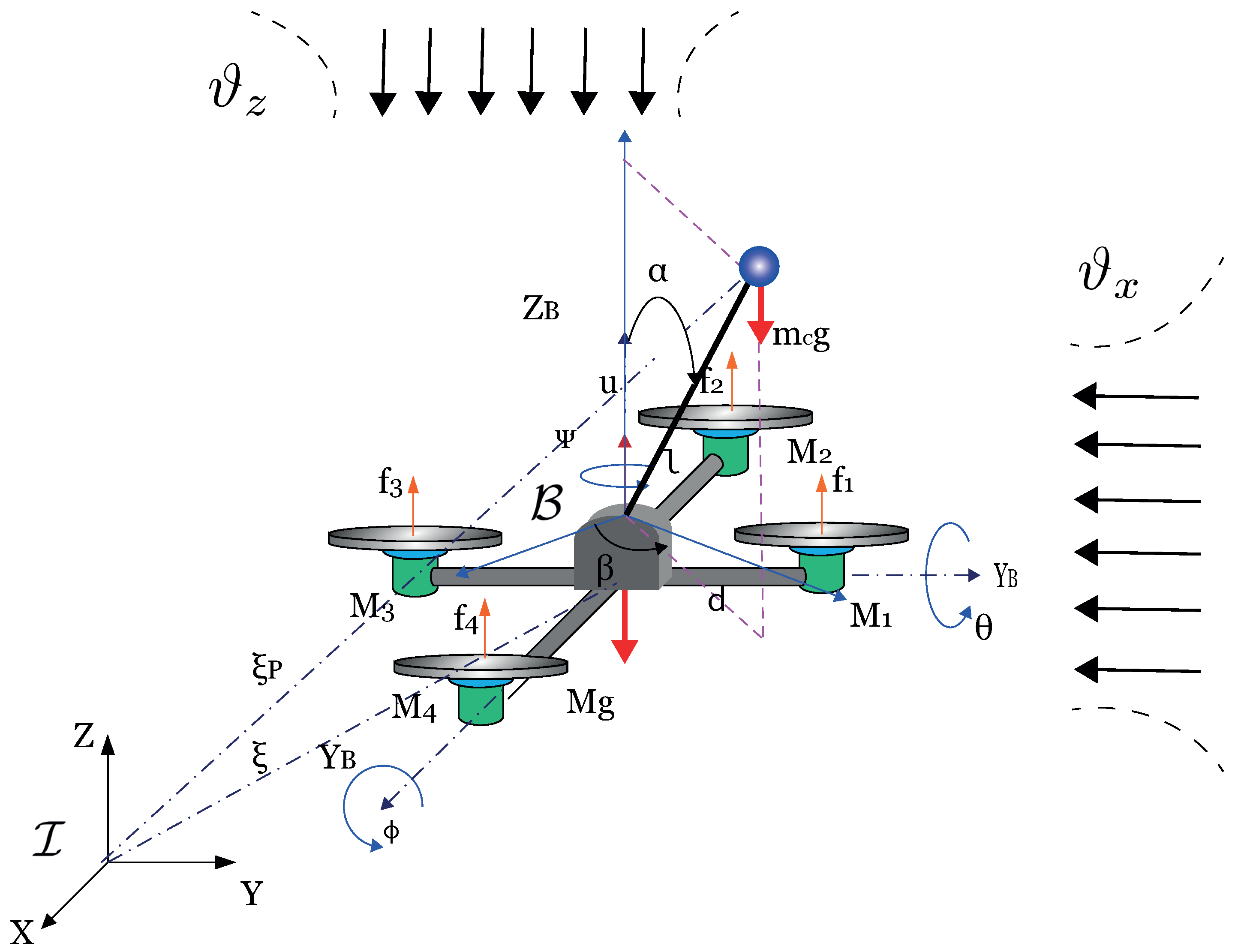
2. Inverted Pendulum on a Quadrotor Model

In Figure 1, a quadrotor with an inverted pendulum is shown. For practical purposes, the system is considered to be subject to external disturbances that may be crosswind disturbances. However, as will be shown later, the term disturbances also consider endogenous disturbances, mainly those associated with dynamics not modeled or neglected in the modeling process. In this sense, the Euler-Lagrange formalism is suggested to obtain the complete model of the inverted pendulum system on a quadrotor.
The Lagrangian of the system is considered as:
L = K Q u a d r o t o r + K P e n d u l u m T Q u a d r o t o r T P e n d u l u m ,
where K Q u a d r o t o r and K P e n d u l u m are the kinetic energy of the quadrotor and el pendulum, while T Q u a d r o t o r and T p e n d u l u m are the potential energy associate to the quadrotor and the pendulum respectively. The definitions of these terms is defined as:
K Q u a d r o t o r = 1 2 M ξ ˙ T ξ ˙ + 1 2 η ˙ T J η ˙ ,
K P e n d u l u m = 1 2 m c ξ ˙ p T ξ ˙ p ,
T Q u a d r o t o r = M g z ,
T P e n d u l u m = m c g ( z + l cos α )
Being ξ = [ x y z ] T R 3 the coordinates of the center of mass of the quadrotor with respect to the inertial frame I . ξ p = ξ + l r with r = [ sin α cos β sin α sin β cos α ] T R 3 the coordinates of the bob mass with respect to the inertial frame. η = [ ϕ θ ψ ] T S 3 the Euler angles of the quadrotor with respect to the frame B , while the J matrix is defined in [19].
Applying the Euler-Lagrange equation as:
d d t L q ˙ L q = u ,
where u = [ f τ 0 0 ] T R 8 represents the force applied to the quadrotor by the propulsion force considering the next definitions f = R F R 3 , being F = [ 0 0 u ] T R 3 , where u = f 1 + f 2 + f 3 + f 4 , while R is a rotation matrix defined in [19]. τ = [ τ ϕ τ θ τ ψ ] T R 3 represent the torque inputs defined as τ ϕ = ( f 2 f 4 ) d , τ θ = ( f 3 f 1 ) d , τ ψ = i = 1 4 τ M i , with τ M i is the torque produced by the motor M i .
A generic form of the full system can be represented by the equation:
M ( q ) q ¨ + C ( q , q ˙ ) q ˙ + G ( q ) = B u
The matrices and vector expressions associated with the previous Equation (7) are as follows, where q = [ x y z ϕ θ ψ α β ] T is the generalized coordinates vector. The development of the full equations was done in Maple software, find the files at https://drive.google.com/drive/folders/1m4ci86XqrfgyvfScftufrJmsl7_2Y7uC (accessed on 19 May 2023).
M ( q ) = ( M + m c ) I 3 × 3 0 3 × 3 Θ 0 3 × 3 I Q 0 3 × 2 Γ 0 2 × 3 Φ , C ( q ˙ , q ) = 0 3 × 3 0 3 × 3 Υ 0 3 × 3 0 3 × 3 0 3 × 2 0 2 × 3 0 2 × 3 Ψ ,
G ( q ˙ , q ) = 0 2 × 1 g ( M + m c ) 0 3 × 1 G μ , B = R e 3 0 3 × 3 0 3 × 1 I 3 × 3 0 2 × 1 0 2 × 3 ,
u = [ f τ 0 0 ] T
where e 3 = [ 0 0 1 ] T , and
Θ = m c l C α C β S α S β C α S β S α C β S α 0 , Γ = m c l C α C β S α S β C α S β S α C β S α 0 T ,
Φ = m c l 2 0 0 m c l 2 S α 2 , G μ = m c l g S α 0 ,
Υ = m c l ( α ˙ S α + β ˙ C α S β ) ( α ˙ C α C β + β ˙ S α ) ( α ˙ S α + β ˙ C α C β ) ( α ˙ C α C β + β ˙ S α ) α ˙ C α 0 ,
Ψ = m c l 2 0 β ˙ S α cos α β ˙ S α C β α ˙ S α C β
To simplify the mathematical model representation, the following notation is used S α = sin α ( t ) , C β = cos β ( t ) , S β = sin β ( t ) , C ϕ = cos ϕ ( t ) , S ϕ = sin ϕ ( t ) , C θ = cos θ ( t ) , S θ = sin θ ( t ) , C ψ = cos ψ ( t ) , S ψ = sin ψ ( t ) is used.

Problem Statement

An output reference trajectory tracking control strategy of the inverted spherical pendulum system on a quadrotor subjected to external disturbances given by crosswind is desired. The control strategy is based on a DESO for the estimation of unknown disturbances given by the neglected non-linear crosswind, as well as, phase variables of the flat outputs which are compensated in the feedback control. It is required that the trajectory tracking errors: e ψ = ψ ψ d , e z = z z d , e F x = F F x d and e F y = F u F y d and α 0 , satisfying the criteria:
e ψ ( t ) ϵ t T 0 ,
e z ( t ) ϵ t T 0 ,
e F x ( t ) ϵ t T 0
e F y ( t ) ϵ t T 0
In which T 0 represents a selected settlement period.

3. Control Strategy

Control techniques used to stabilize the full system are based on the following priority rule. (1) the yaw angle is stabilized via a control, in this case it is desired that ψ ψ d , then consequently controlling the translation movement in height, i.e., z z d . (2) by means of the torques associated with the rotational dynamics, the horizontal translational motion of the quadrotor is controlled, consequently, controlling the swinging movement of the inverted pendulum, this is achieved through a relationship of the states by means of a flat output All the decoupling algebraic process was made in maple software; find the files are at https://drive.google.com/drive/folders/1m4ci86XqrfgyvfScftufrJmsl7_2Y7uC (accessed on 19 May 2023).

3.1. Yaw Control

To carry out the aforementioned control schemes, it is necessary to decouple the model given by Equation (7), where the yaw dynamics result as,
ψ ¨ = τ ψ I ψ + ϑ ψ ,
where ϑ ψ is the term that represents the global perturbation introduced into the yaw dynamics. The DESO is then used as a method for estimating the total disturbance,
ψ ^ ˙ 1 = ψ ^ 2 + λ ψ 3 ( ψ 1 ψ ^ 1 ) , ψ ^ ˙ 2 = u ψ + ϑ ^ ψ 1 + λ ψ 2 ( ψ 1 ψ ^ 1 ) , ϑ ^ ˙ ψ 1 = ϑ ^ ψ 2 + λ ψ 1 ( ψ 1 ψ ^ 1 ) , ϑ ^ ˙ ψ 2 = ρ ψ · sign ( ψ 1 ψ ^ 1 ) ,
where λ ψ 3 , λ ψ 2 , λ ψ 1 and ρ ψ are positive real constants parameters. When the estimation error is defined as e ˜ ψ = ψ 1 ψ ^ 1 , the dynamics of the estimation error introduced by the observer is governed by the following.
e ˜ ψ ( 4 ) + λ ψ 3 e ˜ ψ ( 3 ) + λ ψ 2 e ˜ ¨ ψ + λ ψ 1 e ˜ ˙ ψ + ρ ψ · sign ( e ˜ ψ ) = ϑ ¨ ψ
A characteristic polynomial then denotes the dynamics for the DESO’s tracking error estimation in yaw dynamics, this is
p ψ ( s ) = s 4 + λ ψ 3 s 3 + λ ψ 2 s 2 + λ ψ 1 s + λ ψ 0
The ADRC-DESO output reference in yaw dynamics is given by:
τ ψ = I ψ ψ ¨ d k ψ 1 ( ψ ˙ ψ ˙ d ) k ψ 0 ( ψ ψ d ) ϑ ^ ψ 1 ,
where k ψ 1 , k ψ 0 are positive constants real parameters and I ψ is the moment of inertia.

3.2. Height Control

Decoupling the system (7), the vertical dynamics associated with the height control correspond to
z ¨ = g z u + ϑ z ,
where ϑ z = f z + ϑ z 1 , is the term of total disturbace un the vertical Z axis, and u is the thrust force control input. The term ϑ z 1 corresponds to the exogenous or external unknown disturbance, in this case, a wind gust. The term g z corresponds to the nonlinear terms as a result of decoupling the complete model given by (7), and f z corresponds to nonlinearities associated with the dynamics at height and are defined as,
g z = ( m c ( C ψ S β S ψ C β ) S ϕ ( C ψ C β + S ψ S β ) S θ C ψ S α C α M ( M + m c ) + ( M + m c ) C θ C ϕ m c C α 2 C ϕ C θ M ( M + m c ) ) ,
f z = m c l β ˙ 2 ( C α C α 3 ) + m c l α ˙ 2 C α ( M + m c ) g M + m c ,
The following dynamics describe the DESO for the height dynamics:
z ^ ˙ 1 = z ^ 2 + λ z 3 ( z 1 z ^ 1 ) , z ^ ˙ 2 = u z + ϑ ^ z 1 + λ z 2 ( z 1 z ^ 1 ) , ϑ ^ ˙ z 1 = ϑ ^ z 2 + λ z 1 ( z 1 z ^ 1 ) , ϑ ^ ˙ z 2 = ρ z · sign ( z 1 z ^ 1 ) ,
where λ z 3 , λ z 2 , λ z 1 and ρ z are positive real constants parameters. Given that e ˜ z = z 1 z ^ 1 , the dynamics of the estimation error is by the following:
e ˜ z ( 4 ) + λ z 2 e ˜ z ( 3 ) + λ z 1 e ˜ ¨ z + λ z 0 e ˜ ˙ z + ρ z · sign ( e ˜ z ) = ϑ ¨ z
The following characteristic polynomial then, denotes the dynamics for estimating the DESO’s tracking error in height dynamics,
p z ( s ) = s 4 + λ z 3 s 3 + λ z 2 s 2 + λ z 1 s + λ z 0
For height dynamics (17), the following describes the ADRC-based DESO output reference trajectory tracking controller.
u = z ¨ d k z 1 ( z ˙ z ˙ d ) k z 0 ( z z d ) ϑ ^ z 1 g z

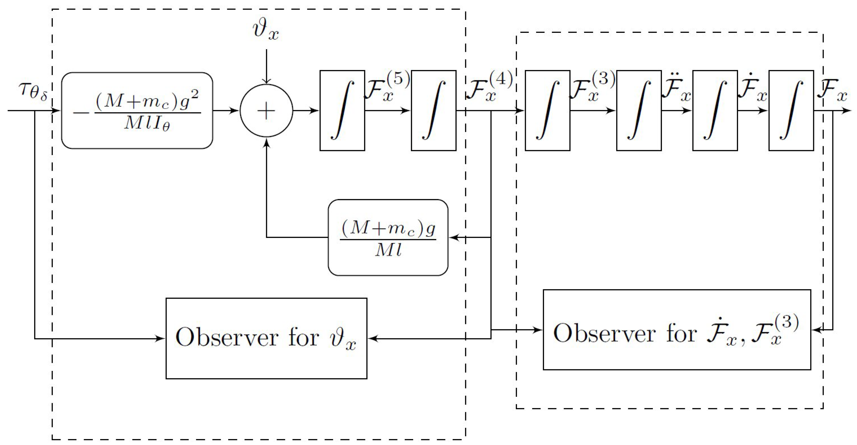
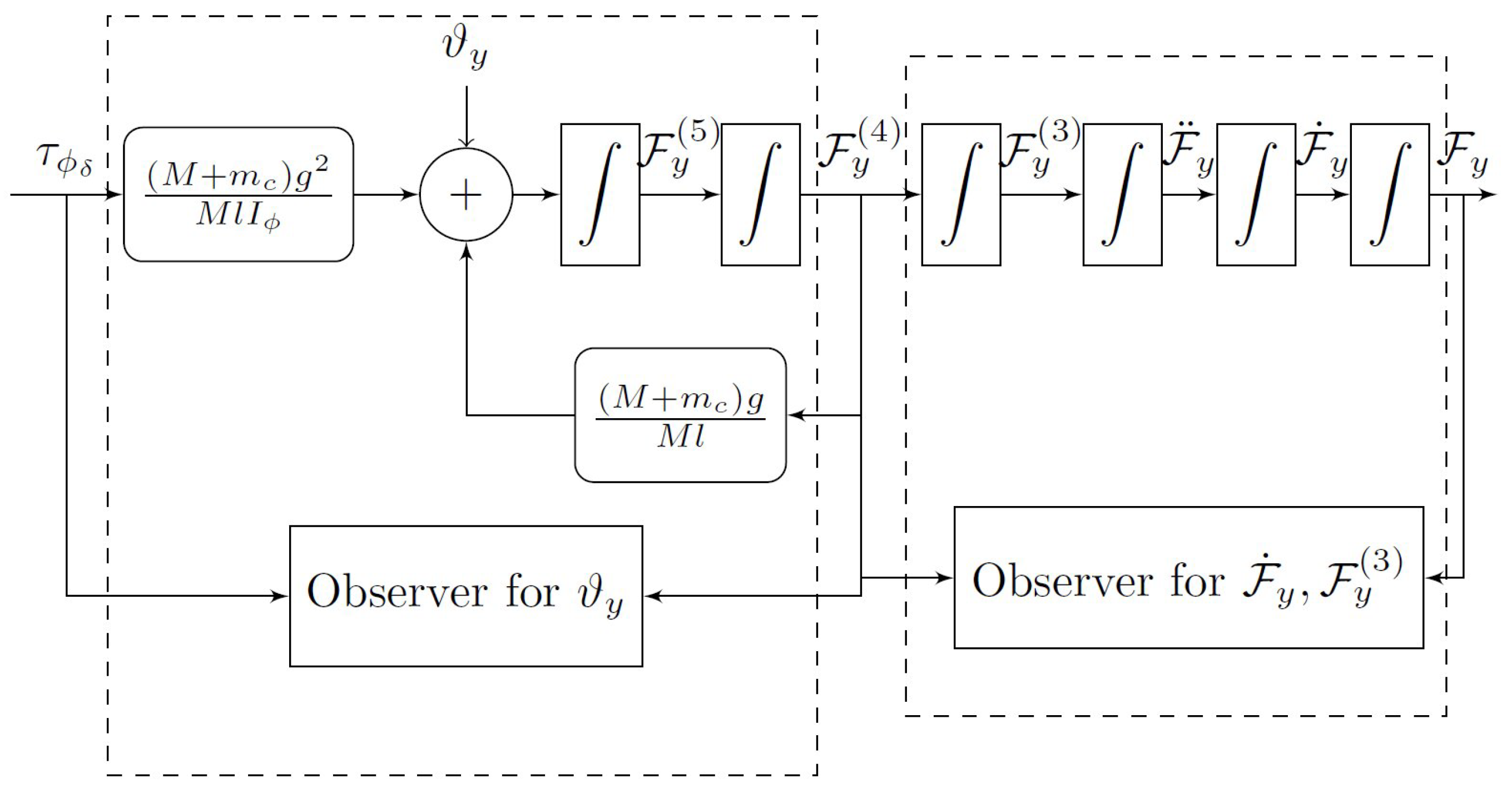
3.3. Horizontal Position Control

The horizontal dynamics of the inverted pendulum system on a quadrotor is governed by the rotational dynamics of the quadrotor which is controlled by the control inputs associated with the torques due to the thrust forces of the motors. The translational dynamics of the quadrotor is associated in a cascade scheme together with the rotational dynamics; this is, to move the quadrotor horizontally it is necessary to generate an effect on the translational dynamics, and in turn the translational dynamics allows to control the balance of the inverted pendulum. To achieve this in 3-D space, it is necessary to decouple the complete system in a translation dynamic around the X axis with β = 0 and another around the Y axis considering that β = π / 2 , provided that it has been fulfilled ψ 0 and z z d have been accomplished. Making use of the symmetry of the system and considering small movements in the rotational dynamics, both dynamics can be linearized on the X and Y axis around the equilibrium points ( x ( t ) , y ( t ) , z ( t ) , ϕ ( t ) , θ ( t ) , α ( t ) ) = ( x ¯ , y ¯ , z ¯ , 0 , 0 , 0 ) and u ( t ) = u ¯ = ( M + m c ) g , τ ¯ ϕ = 0 , τ ¯ θ = 0 . The linearized and decoupled model around X axis is given by
x ¨ δ = ( M + m c ) g θ δ m c g α M ,
θ ¨ δ = τ θ δ I θ ,
α ¨ δ = ( M + m c ) g M l ( α δ θ δ ) ,
while the decoupled linearized model for the Y frame is represented by,
y ¨ δ = ( M + m c ) g ϕ δ m c g α M ,
ϕ ¨ δ = τ ϕ δ I ϕ ,
α ¨ δ = ( M + m c ) g M l ( ϕ δ α δ )
A set of flat outputs are defined [17,20,21].
F x = x δ + l α δ ,
F y = y δ + l α δ
The dynamics of translation around the X axis with the F x shows the following relationship:
F x = x δ + l α δ ,
F ˙ x = x ˙ δ + l α ˙ δ ,
F ¨ x = g α δ ,
F x ( 3 ) = g α ˙ δ ,
F x ( 4 ) = ( M + m c ) g 2 M l ( α δ θ δ ) ,
F x ( 5 ) = ( M + m c ) g 2 M l ( α ˙ δ θ ˙ δ ) ,
F x ( 6 ) = ( M + m c ) g 2 I θ M l τ θ δ + ( M + m c ) g M l F ( 4 ) ,
Also, the following relationships between the system state variables and the F y flat output are associated with the Y axis and its time derivatives.
F y = y δ + l α δ ,
F ˙ y = y ˙ δ + l α ˙ δ ,
F ¨ y = g α δ ,
F y ( 3 ) = g α ˙ δ ,
F y ( 4 ) = ( M + m c ) g 2 M l ( ϕ δ α δ ) ,
F y ( 5 ) = ( M + m c ) g 2 M l ( ϕ ˙ δ α ˙ δ ) ,
F y ( 6 ) = ( M + m c ) g 2 I θ M l τ ϕ δ + ( M + m c ) g M l F ( 4 )
Because of the symmetric of the quadrotor, both dynamics of the newly formed linear system have the same structure, and the Equations (38) and (45) show that the new system has a relative degree six. The Figure 2 and Figure 3 show how a DESO and a Luenberger observer are used to estimate the phase variables and unknown uncertainties along the X and Y axes, respectively.
As mentioned above, due to the symmetry of the system, the structure of both lateral dynamics is identical; thus, only one case is presented to avoid rewriting the same observer’s system, which can be applied to the translational motion around X and Y axis. The following can be proposed as an appropriate Luenberger observer for the first stage of the horizontal position.
F ^ ˙ 1 = F ^ 2 + λ 3 ( F 1 F 1 ^ ) , F ^ ˙ 2 = F ^ 3 + λ 2 ( F 1 F 1 ^ ) , F ^ ˙ 3 = F ^ 4 + λ 1 ( F 1 F 1 ^ ) , F ^ ˙ 4 = F 5 + λ 0 ( F 4 F 4 ^ ) ,
λ 3 , λ 2 , λ 1 , λ 0 are positive real constants parameters. A DESO can observe the unknown total disturbance in the second stage in the form
F ^ ˙ 5 = F ^ 6 + λ 3 ( F 5 F 5 ^ ) , F ^ ˙ 6 = u F + ϑ ^ x + λ 2 ( F 5 F 5 ^ ) , ϑ ^ ˙ x 1 = ϑ ^ x 2 + λ 1 ( F 5 F 5 ^ ) , ϑ ^ ˙ x 2 = ρ F · sign ( F 5 F 5 ^ )
ρ F real positive constant. Given that e ˜ 1 = F 1 F ^ 1 , the dynamics of the DESO estimation error is governed by:
e ˜ 1 ( 4 ) + λ 3 e ˜ 1 ( 3 ) + λ 2 e ˜ ¨ 1 + λ 1 e ˜ ˙ 1 + λ 0 e ˜ 1 = 0 ,
and with e ˜ 5 = F 5 F ^ 5 ,
e ˜ 5 ( 4 ) + λ 3 e ˜ 5 ( 3 ) + λ 2 e ˜ ¨ 5 + λ 1 e ˜ ˙ 5 + ρ F · sign ( e ˜ 5 ) = ϑ ¨ F ,
The following expression represents the property characteristic polynomial associated with the estimated error dynamic of the tracking prediction error by both observers in the estimation factor. The characteristic polynomial of the DESO is given by:
p F = s 4 + λ 3 s 3 + λ 2 s 2 + λ 1 s + λ 0
Finally, the feedback control compensated the total disturbances for both, dynamic motion on the X and Y axes respectively associate to the torque are shown below.
τ θ = M l I θ ( M + m c ) g 2 ( k 5 ( F ^ x ( 5 ) F x d ( 5 ) ) k 4 ( F x ( 4 ) F x d ( 4 ) ) k 3 ( F ^ x ( 3 ) F x d ( 3 ) ) k 2 ( F ¨ x F ¨ x d ) k 1 ( F ^ ˙ x F x d ˙ ) k 0 ( F x F x d ) ϑ ^ x + F x d ( 6 ) ) + I θ g F x ( 4 ) ,
and the equation of motion along the Y-axis is given by:
τ ϕ = M l I ϕ ( M + m c ) g 2 ( k 5 ( F ^ y ( 5 ) F y d ( 5 ) ) k 4 ( F y ( 4 ) F y d ( 4 ) ) k 3 ( F ^ y ( 3 ) F y d ( 3 ) ) k 2 ( F ¨ y F ¨ y d ) k 1 ( F ^ ˙ y F ˙ y d ) k 0 ( F F y d ) ϑ ^ y + F d ( 6 ) ) + I ϕ g F y ( 4 )

4. Convergence Analysis

This section shows the convergence analysis of DESO and feedback controls based on Lyapunov’s first theorem.

4.1. Discontinuous Extended State Observer

Theorem 1. 
Let us assuming that small movements are considered in the rotational dynamics of the quadrotor, that the inverted pendulum starts from an initial condition close to the unstable equilibrium point and that, in addition, the perturbations are bounded and differentiable. If the coefficients λ z 0 , , λ z 2 , λ ψ 0 , , λ ψ 2 and λ 0 , , λ 3 associated with the characteristic polynomials of the DESO design are chosen such that for N > > 0 , all the roots are located to the left of the complex plane C on the line { s C | Re ( s ) N } . Then the estimation errors e ˜ ψ , e ˜ z 1 , e ˜ F 1 and e ˜ F 4 converge globally and asymptotically towards a ball of radius ρ given by S ( 0 , r ) , and the estimation variables ϑ ^ ψ , ϑ ^ z , ϑ ^ x , ϑ ^ y converge towards ϑ ψ , ϑ z , ϑ x , ϑ y .
Proof. 
Let e ˜ = [ e ˜ 1 , , e ˜ 4 ] T stand for the phase variables in each (14), (21) and (49) given system, These systems may be expressed generically as
e ˜ ˙ = A e e ˜ + b ϑ ˙ ρ · sign ( e ˜ ) ,
where
A e = 0 1 0 0 0 0 1 0 0 0 0 1 0 λ 1 λ 2 λ 3 ,
b = 0 0 0 1 T
Given the largest eigenvalue of A e this is such that | Re ( σ m a x ( A e ) ) | N . This means that there is a constant, symmetric, positive matrix P that guarantees a solution to the Lyapunov equation for any given Q = Q T > 0 .
A e T P + P A e = Q
Choosing a Lyapunov Function Candidate.
V ( e ˜ ) = 1 2 e ˜ T P e ˜ ,
for the resultant closed-loop system and taking the derivative with respect to time of V ( e ˜ ) ,
V ˙ ( e ˜ ) = 1 2 e ˜ T ( A e T P + PA e ) e ˜ + e ˜ T Pb ( ϑ ¨ ρ · sign ( e ˜ ) ) ,
V ˙ ( e ˜ ) e ˜ 2 P | Re ( σ m a x ( A e ) ) | e ˜ P ( ρ · sign ( e ˜ ) ϑ ¯ ) ,
V ˙ ( e ˜ ) e P | Re ( σ m a x ( A e ) ) | e ϑ ¯
Thus, outside the sphere, this function has a strictly negative value.
S ( 0 , r ) = e R 4 | e ρ = ϑ ¯ | Re ( σ m a x ( A e ) ) | ϑ ¯ N
As a result, no path entering S ( 0 , ρ ) will never leave it. The ultimate bounding sphere’s radius S ( 0 , r ) along e ˜ decreases with the dominant eigenvalue’s real component of A e increases ( | Re ( σ m a x ( A e ) ) | ).
To express the estimation error given by (46), the Luenberger observer can be formulated as
e ˜ ˙ 1 = A e 1 e ˜ 1 ,
where
A e 1 = 0 1 0 0 0 0 1 0 λ 0 λ 1 λ 2 λ 3
Given C as the complex plane, all the roots of this system lie on the line’s left side { s C | Re ( s ) N } . The error estimators e ˜ 1 thus tend to converge asymptotically to zero. □

4.2. The Disturbance Canceling Controller
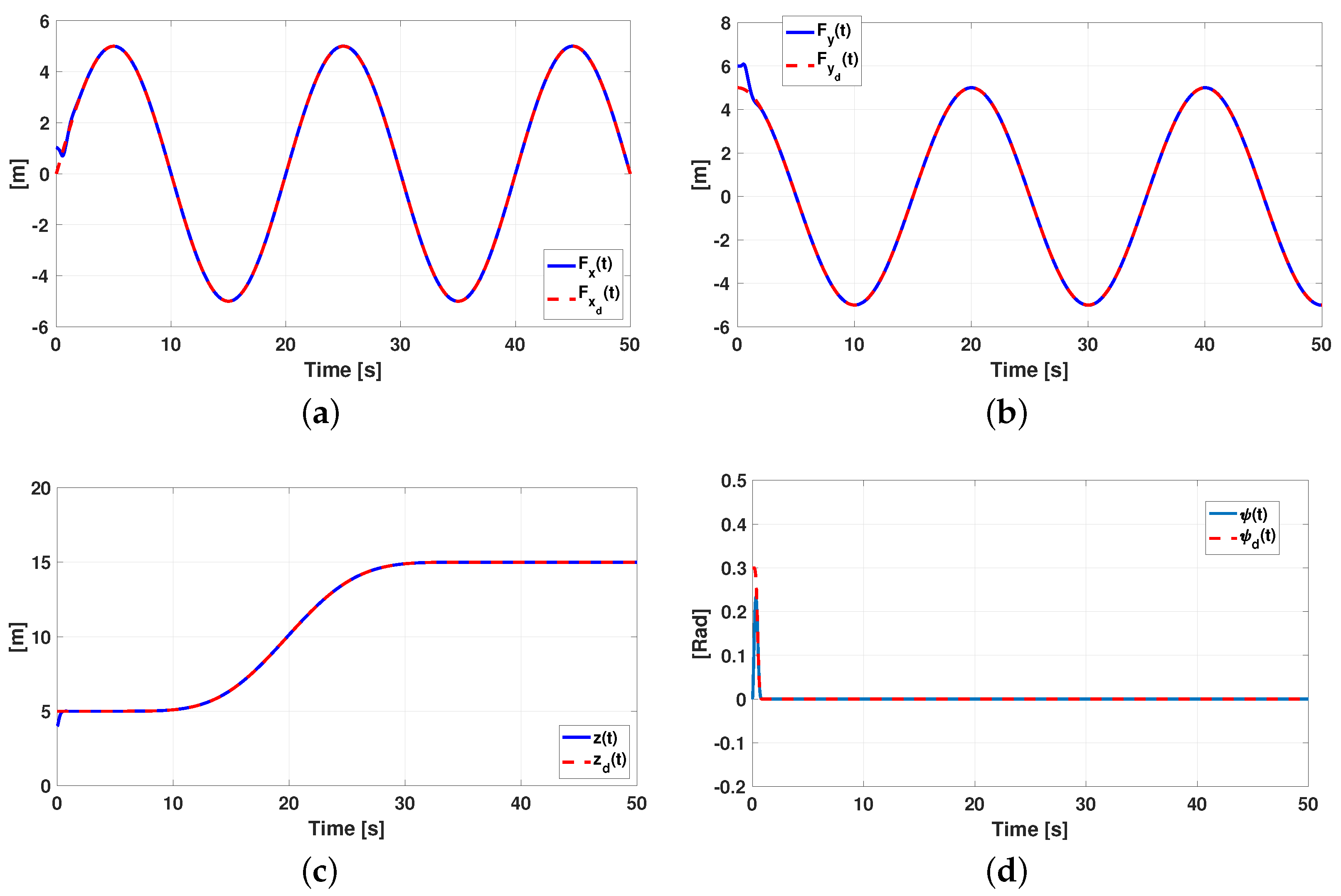
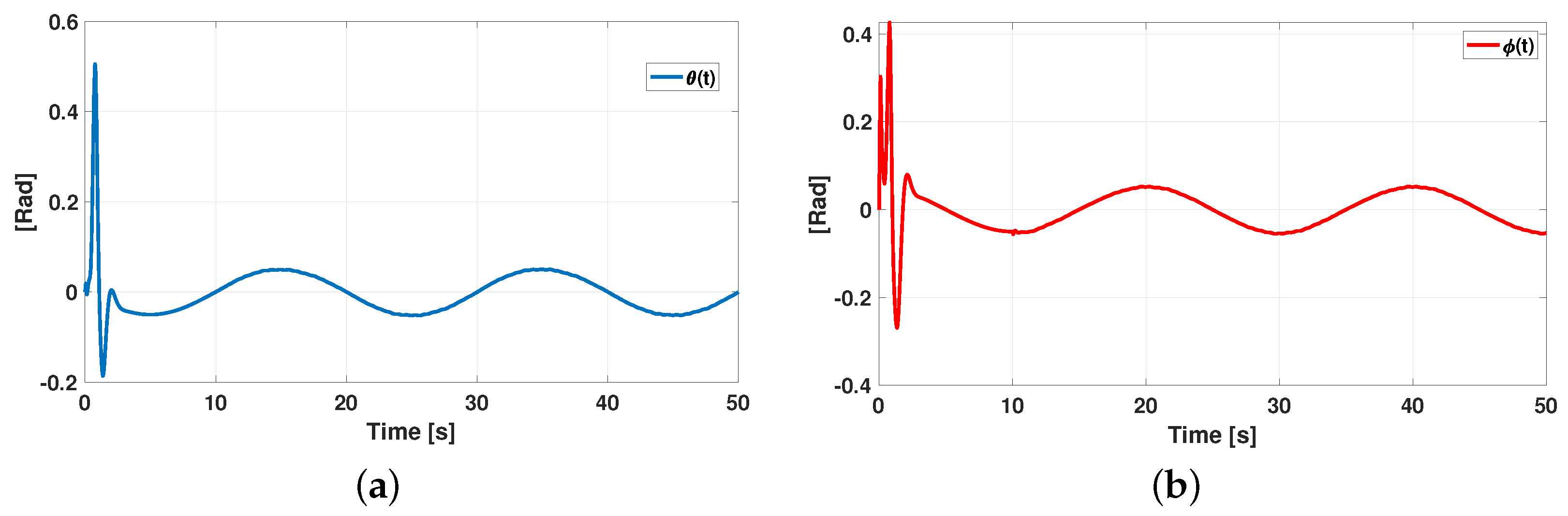
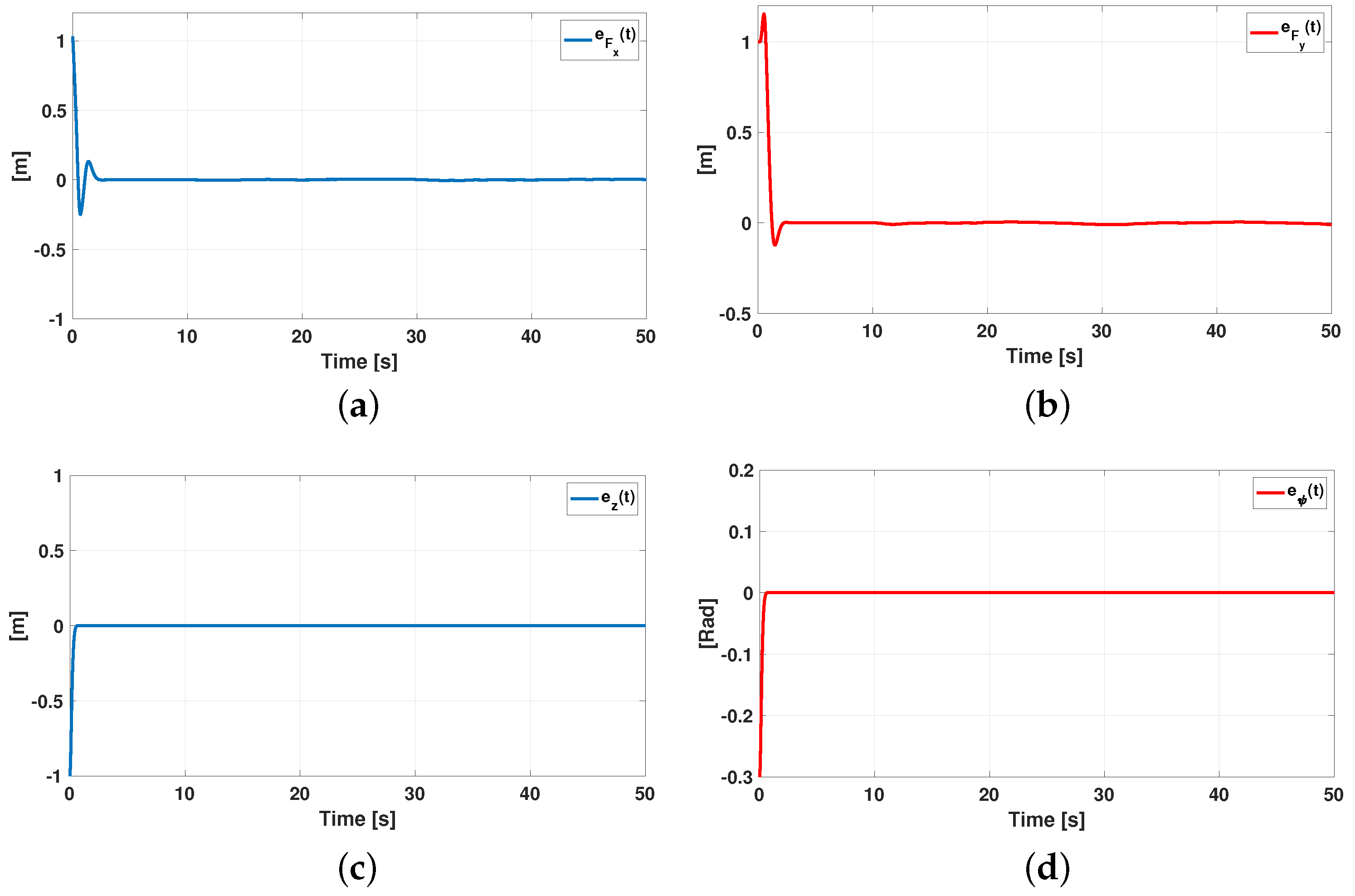
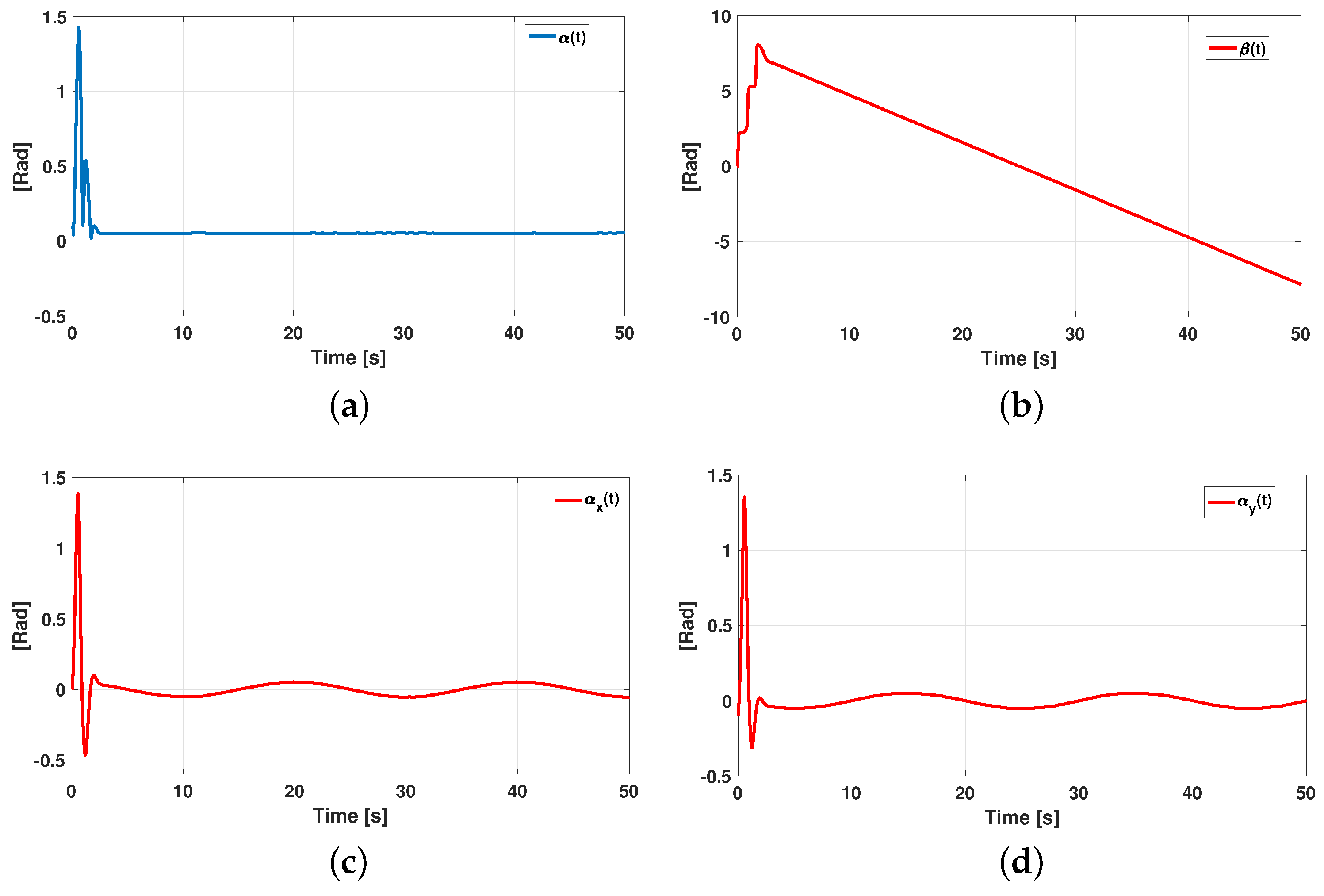
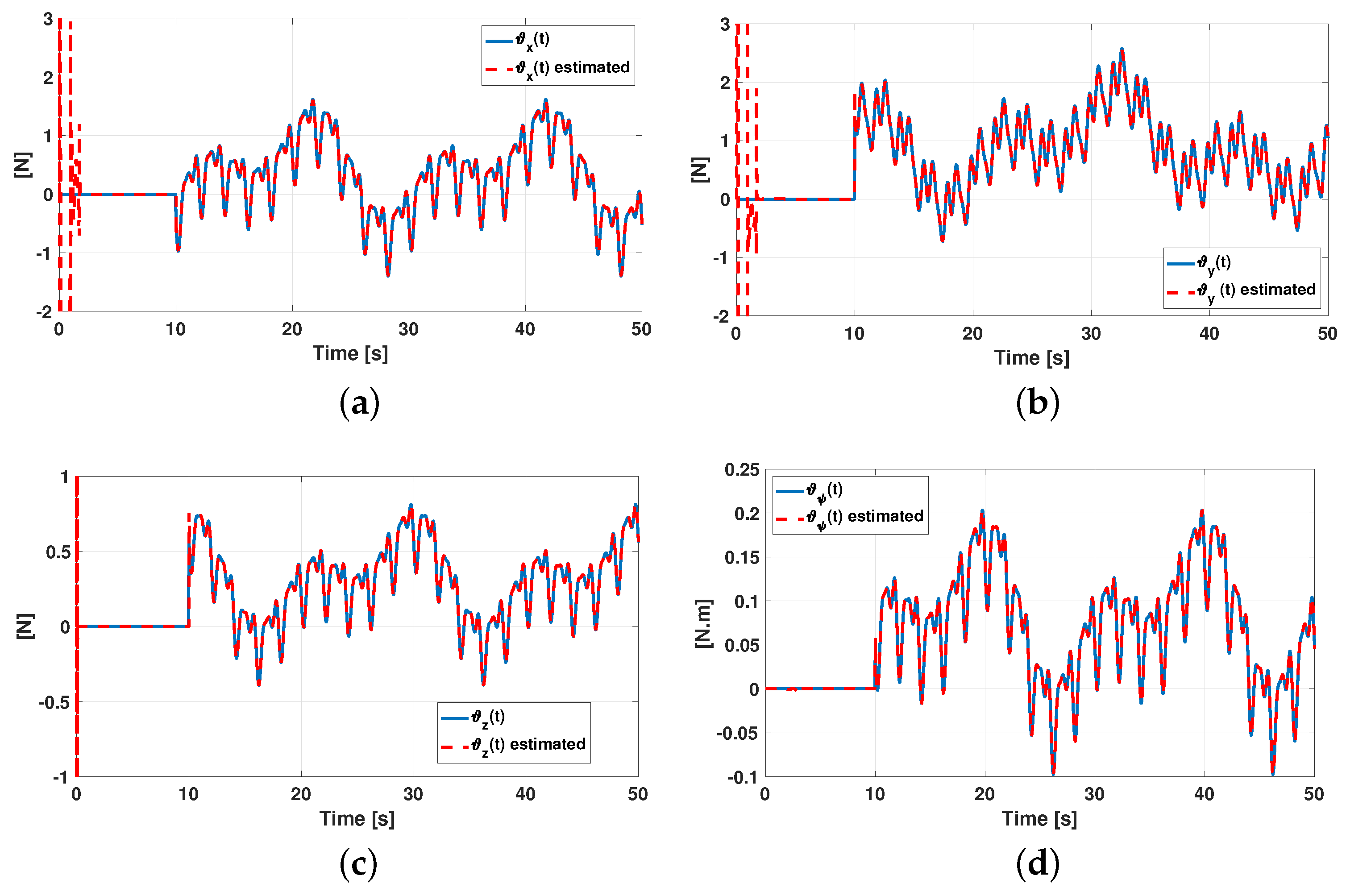
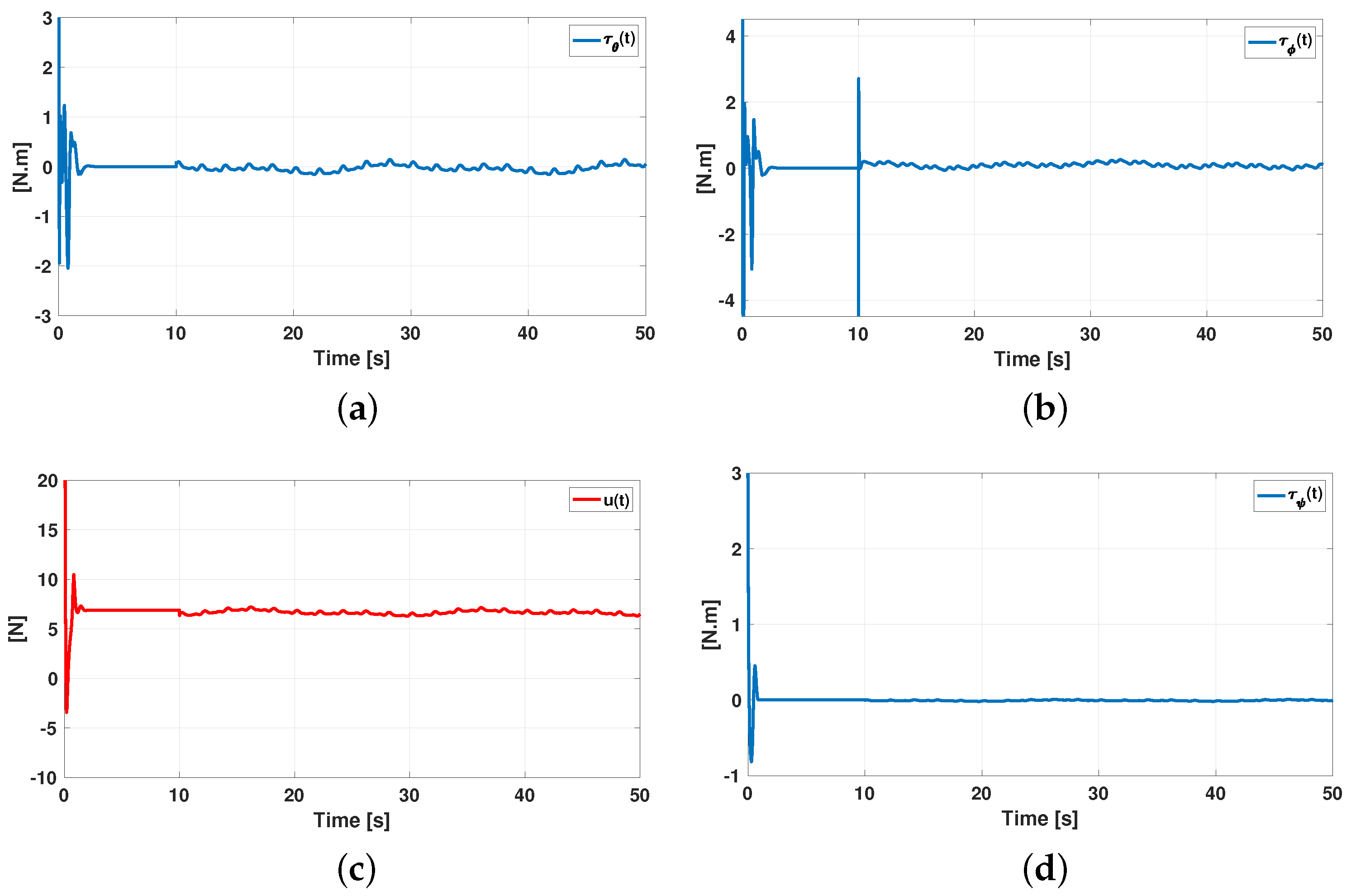
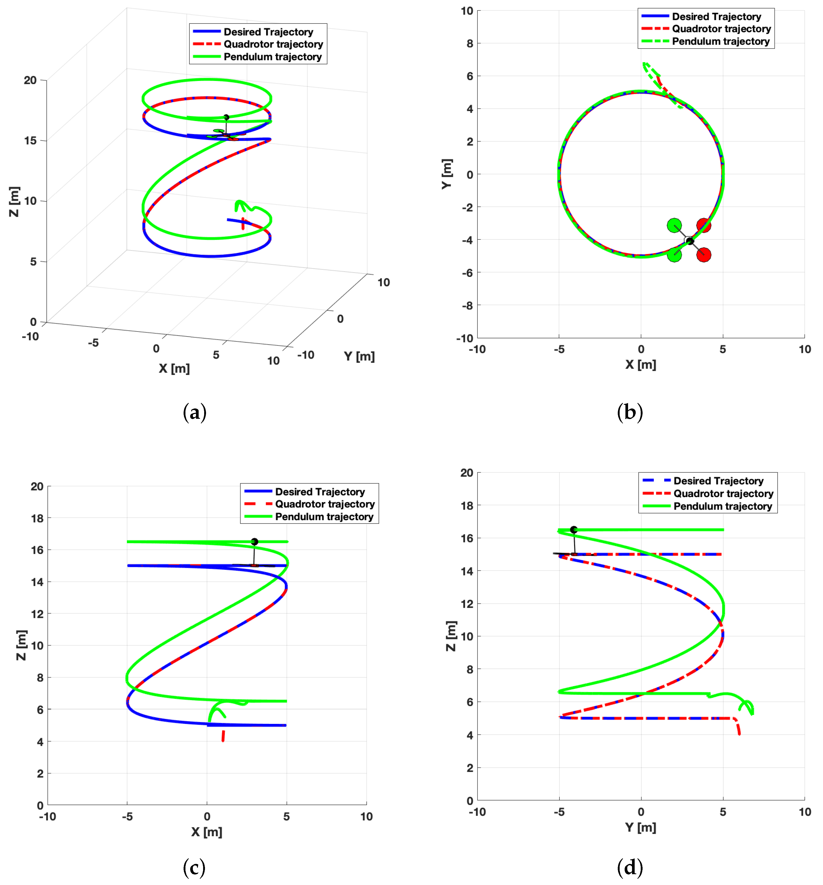
According to the feddback controls (16), (23), (51) and (52) for the yaw, height, and horizontal trajectory tracking, respectively, defining the trajectory tracking errors e ψ = ψ ψ * , e z = z z * and e F = F F * , respectively, the closed-loop system of each dynamics are given by
e ¨ ψ + k ψ 1 e ˙ ψ + k ψ 0 e ψ + ( ϑ ψ ϑ ^ ψ ) = 0 ,
e ¨ z + k z 1 e ˙ z + k z 0 e z + ( ϑ z ϑ ^ z ) = 0 ,
e F ( 6 ) + k 5 e F ( 5 ) + k 4 e F ( 4 ) + k 3 e F ( 3 ) + k 2 e ¨ F + k 1 e ˙ F + k 0 e F + ( ϑ F ϑ ^ F ) = 0
These closed-loop dynamics have a generic representation expressed in a linear state space as:
e ˙ = Ae + B ( ϑ ϑ ^ ) ,
where e = [ e , e ˙ , , e ( n ) ] T is a state vector, taking the following values: e = e ψ , with ϑ = ϑ ψ , n = 2 for (61); e = e z , with ϑ = ϑ z , and n = 2 for (62); e = e F , with ϑ = ϑ F for (63), and n = 6 .
Theorem 2. 
Let the set of coefficients k z 0 , k z 1 and k 0 , k 5 are chosen in such a way that the phase space for output tracking errors ( e , e ˙ , , e ( n 1 ) ) provided by the disturbance rejection feedback controllers (16), (23), (51) and (52), guides the trajectory tracking error of the controlled systems ψ, z, F x and F y toward a small desired region of the origin and are chosen such that,
p ψ = s 2 + k ψ 1 s + k ψ 0 ,
p z = s 2 + k z 1 s + k z 0 ,
p F = s 6 + k 5 s 5 + k 4 s 4 + k 3 s 3 + k 2 s 2 + k 1 s + k 0
These polynomials are Hutwitz if and only if defined the number N > > 0 , and their roots lie far enough on the left side of the imaginary axis in the field { s C | Re ( s ) N } . Then, the trajectories of the tracking error e = e ψ , e = e z , e = e F x and e = e F y globally converge to a ball S ( 0 , ρ ) with radius ρ, as small as desired.
Proof. 
The previous theorem states that the generic system (64), the term ( ϑ ϑ ^ ) and e , e ˙ , , e n 1 evolve in a small as desired neighborhood of the origin in terms of the estimation error of the disturbance. It can be said that the estimation error ϑ ϑ ^ = e ϑ e ¯ ϑ is bounded in this sense. A candidate Lyapunov function is proposed using the same evidence presented in Theorem 1, this is.
V ( e ) = 1 2 e T P e ,
whose the derivative with respect to time takes the form,
V ˙ ( e ) = 1 2 e T ( A T P + PA ) e + e T P B e ϑ ,
V ˙ ( e ) e 2 P | Re ( σ m a x ( A ) ) | + e ¯ ϑ e P ,
V ˙ ( e ) e P | Re ( σ m a x ( A ) ) | e e ¯ ϑ
V ˙ ( e ) is strictly non positive anywhere outside the ball,
S ( 0 , ρ ) = e R n | e ρ = e ¯ ϑ | Re ( σ m a x ( A ) ) |
Thus, if we substitute each one of the dynamics of movement of the system (12), (17), (38) and (45) the trajectory tracking errors of the full system converges towards the inside of the sphere of radius S ( 0 , ρ ) , the larger the quantity | Re ( σ m a x ( A ) ) | . The sphere’s radius is smaller. □

5. Numerical Result

Numerical simulations were carried out considering the nonlinear system given by (7). The parameters of the quadrotor UAV and the inverted pendulum are summarized in Table 1.
The parameters for the yaw and height dynamics of the DESO are selected according to λ ψ 1 = λ z 1 = 4 ζ ω n 3 , λ ψ 2 = λ z 2 = 4 ζ 2 ω n 2 + 2 ω n 2 , λ ψ 3 = λ z 3 = 4 ζ ω n , and feedback control k ψ 0 = k z 0 = ω n c 2 , k ψ 1 = k z 1 = 2 ζ c ω n c , with ω n = 500 , ζ = 0.9 , and ω n c = 10 , ζ c = 0.9 . The parameters for lateral or horizontal dynamics are selected as λ 0 = ω n 2 , λ 1 = 4 ζ ω n 3 , λ 2 = 4 ζ 2 ω n 2 + 2 ω n 2 , λ 3 = 4 ζ ω n , and the feedback control k 0 = ω n c 6 , k 1 = 6 ζ c ω n c 5 , k 2 = 12 ω n c 4 ζ c 2 + 3 ω n c 4 , k 3 = 8 ω n c 3 ζ c 3 + 12 ω n c 3 ζ c , k 4 = 12 ω n c 2 ζ c 2 + 3 ω n c 2 , k 5 = 6 ω n c ζ c with ω n = 500 , ζ = 0.9 , and ω n c = 7 , ζ c = 0.9 . These parameters are chosen in a suitable way so that their corresponding polynomials are Hurwitz.
In Figure 4 the behavior of the trajectory tracking of the quadrotor-inverted pendulum system are shown. The behavior of the variables ψ , z, corresponding to the yaw and height dynamics of the quadrotor are shown in Figure 4d,c, while, the flats outputs associated to the horizontal translational dynamics of the quadrotor are shown in Figure 4a,b.
Figure 5 shows the behavior of the attitude angles of the quadrotor. In Figure 5a,b the pitch angle and teh roll angle associated with the rotational dynamics of the quadrotor are shown.
The trajectory tracking error e ψ , e z , e F x and e F y associated to the quadtortor are shown in Figure 6. Figure 6a,b show the behavior of the horizontal translations dynamic of the quadrotor on the X Z and Y Z reference frame respectively. Figure 6c,d the trajectory tracking error in height and yaw dynamics are shown. All the errors converge to zero.
Figure 7 shows the behavior of the spherical inverted pendulum on a quadrotor. In Figure 7a the behavior of α angle is shown, this angle goes to zero keeping the inverted pendulum in an unstable vertical position while a trajectory tracking of the quadrotor is taking place. Figure 7b shows the behavior of β angle, this angle describes the translation of the bob with respect to the Z B . Figure 7c,d shows the angle with respect to the Y Z and X Z frame, respectively.
External disturbances, such as wind gusts in vertical, horizontal, and rotational motion in yaw, are randomly generated in simulation and injected into the model. Figure 8 shows the disturbances injected after ten seconds of simulation. Figure 8a,b shows the disturbance in the horizontal on the X and Y axis. Figure 8c shows the disturbance injected in the vertical dynamics, while Figure 8d shows the disturbance in yaw dynamics.
The behavior of feedback control signals with compensation of the disturbance are depicted in Figure 9. Figure 9a,b show the control signals associated to the pitch and roll angles of the quadrotor. Figure 9c,d shows the behavior of the control signals in height and yaw quadrotor’s dynamics. The effect of the disturbances injected to the quadrotor after ten seconds of simulation are reflected in the control signals.
Figure 10 shows a virtual behavior of the full system with a trajectory tracking control scheme. Figure 10a illustrates the three-dimensional trajectory tracking of the quadrotor with the spherical inverted pendulum, where it is observed that the system starts from an initial condition different from the desired trajectory, and by the action of the feedback control with compensation of the disturbances it converges towards the desired trajectory. In addition, the behavior of the inverted pendulum is observed, whose kinematics is obtained from the numerical solutions of the elements α and β , demonstrating that β does not converge to zero. Figure 10b shows the projections in the X Y frame, and Figure 10c,d represent the behavior of the system in the coordinate systems X Z and Y Z .

6. Conclusions

In this paper, a discontinuous extended state observer-based differential flatness to the trajectory tracking problem of the spherical inverted pendulum attached on a quadrotor UAV in three-dimensional space is presented. The full nonlinear model of the system is obtained by the Euler-Lagrange formalism considering as control input the torques over the Euler angles and the thrust force due to the propels of the quadrotor. This issue requires considering small movements of the quadrotor-inverted pendulum system, which by means of a linearization around an equilibrium point allows for reducing the complexity of the full model. Taking into account the differential flatness property of the linear model, a set of new outputs are proposed (flat outputs) which allow the design of an active disturbance rejection control in each control dynamics, more precisely, roll, pitch, yaw, and in height dynamic. The proposed solutions guarantee accurate estimation of the total disturbance which are used to compensate for their effects on feedback control, as well as, guarantee trajectory tracking of the system with a minimum bounded error as it is shown in the stability analysis. Finally, numerical simulations are shown to validate the control strategy. An important aspect to highlight in our work is the solution to the β angle of the system, which is projected on the earth, i.e., in the X Y frame. This angle, unlike the works reported in the literature where the problem of a suspended load is addressed, never converges to zero, the angle that converges to zero guaranteeing the stability of the inverted pendulum is the α angle. On the other hand, there are few works that address the problem of the inverted pendulum in three-dimensional space, for example, Hehn M. et al. [3] where, unlike our work, the authors propose a change of variable that does not involve the alpha and beta angles, Rather, they propose to obtain the coordinates of the pendulum on the frame of reference in the body, thus avoiding terms that involve angles of oscillation; however, the model they propose is very limited. Villaseñor Rios et al. [14] also address this case, where the problem is mainly studied in two dimensions, considering a particular case of the full model in three dimensions, and also proposing a well-known extended state observer to estimate the external disturbance.

Author Contributions

Conceptualization, A.H.M.-V.; methodology, A.H.M.-V., R.C.-L., H.S.-R.; software, A.H.M.-V.; validation, R.C.-L., A.E.R.-M., H.S.-R.; formal analysis, A.H.M.-V., R.C.-L., H.S.-R.; investigation, A.H.M.-V., R.C.-L.; resources, R.C.-L.; data curation, R.C.-L., A.E.R.-M., H.S.-R.; writing—original draft preparation A.H.M.-V., R.C.-L., H.S.-R.; writing—review and editing, A.H.M.-V., R.C.-L., A.E.R.-M., H.S.-R.; visualization, A.H.M.-V., R.C.-L., A.E.R.-M., H.S.-R.; supervision R.C.-L., A.E.R.-M., H.S.-R.; project administration, R.C.-L.; funding acquisition, A.H.M.-V., R.C.-L., A.E.R.-M., H.S.-R. All authors have read and agreed to the published version of the manuscript.

Funding

Research partially supported by Conahcyt Project CB-254329.

Institutional Review Board Statement

Not applicable.

Informed Consent Statement

Not applicable.

Data Availability Statement

Not applicable.

Acknowledgments

This work was supported by the Consejo Nacional de Humanidades, Ciencias, Tecnologías e Innovación (Conahcyt) and by CINVESTAV-IPN.

Conflicts of Interest

The authors declare that there is no competing financial interest or personal relationship that could have appeared to influence the work reported in this paper.

References

  1. Israilov, S.; Fu, L.; Sánchez-Rodríguez, J.; Fusco, F.; Allibert, G.; Raufaste, C.; Argentina, M. Reinforcement learning approach to control an inverted pendulum: A general framework for educational purposes. PLoS ONE 2023, 18, e0280071. [Google Scholar] [CrossRef] [PubMed]
  2. He, B.; Wang, S.; Liu, Y. Underactuated robotics: A review. Int. J. Adv. Robot. Syst. 2019, 16, 1729881419862164. [Google Scholar] [CrossRef]
  3. Hehn, M.; D’Andrea, R. A flying inverted pendulum. In Proceedings of the 2011 IEEE International Conference on Robotics and Automation, Shanghai, China, 9–13 May 2011; pp. 763–770. [Google Scholar] [CrossRef]
  4. Krafes, S.; Chalh, Z.; Saka, A. Vision-based control of a flying spherical inverted pendulum. In Proceedings of the 2018 4th International Conference on Optimization and Applications (ICOA), Mohammedia, Morocco, 26–27 April 2018; pp. 1–6. [Google Scholar] [CrossRef]
  5. Nayak, A.; Banavar, R.N.; Maithripala, D.H.S. Stabilizing a spherical pendulum on a quadrotor. Asian J. Control 2021, 24, 1112–1121. [Google Scholar] [CrossRef]
  6. Ibuki, T.; Tadokoro, Y.; Fujita, Y.; Sampei, M. 3D inverted pendulum stabilization on a quadrotor via bilinear system approximations. In Proceedings of the 2015 IEEE Conference on Control Applications (CCA), Sydney, Australia, 21–23 September 2015; pp. 513–518. [Google Scholar] [CrossRef]
  7. de Almeida, M.M.; Raffo, G.V. Nonlinear Balance Control of an Inverted Pendulum on a Tilt-rotor UAV. IFAC-PapersOnLine 2015, 48, 168–173. [Google Scholar] [CrossRef]
  8. Yang, Y.; Zhang, D.; Xi, H.; Zhang, G. Anti-swing control and trajectory planning of quadrotor suspended payload system with variable length cable. Asian J. Control 2022, 24, 2424–2436. [Google Scholar] [CrossRef]
  9. Abadi, A.; Amraoui, A.E.; Mekki, H.; Ramdani, N. Robust tracking control of quadrotor based on flatness and active disturbance rejection control. IET Control Theory Appl. 2020, 14, 1057–1068. [Google Scholar] [CrossRef]
  10. Oloo, J. Effect of loss of control effectiveness on an inverted pendulum balanced on a moving quadrotor. Heliyon 2023, 9, e14494. [Google Scholar] [CrossRef] [PubMed]
  11. Nasir, A.N.K.; Razak, A.A.A. Opposition-based spiral dynamic algorithm with an application to optimize type-2 fuzzy control for an inverted pendulum system. Expert Syst. Appl. 2022, 195, 116661. [Google Scholar] [CrossRef]
  12. Siravuru, A.; Sreenath, K. Nonlinear Control using Coordinate-free and Euler Formulations: An Empirical Evaluation on a 3D Pendulum. IFAC-PapersOnLine 2020, 53, 8847–8852. [Google Scholar] [CrossRef]
  13. Yang, W.; Reis, J.; Silvestre, C. Saturated Nonlinear Trajectory Tracking Controller for Inverted Pendulum on a Quadrotor. In Proceedings of the 2022 41st Chinese Control Conference (CCC), Hefei, China, 25–27 July 2022; pp. 1–7. [Google Scholar] [CrossRef]
  14. Villaseñor Rios, C.A.; Luviano-Juárez, A.; Lozada-Castillo, N.B.; Carvajal-Gámez, B.E.; Mújica-Vargas, D.; Gutiérrez-Frías, O. Flatness-Based Active Disturbance Rejection Control for a PVTOL Aircraft System with an Inverted Pendular Load. Machines 2022, 10, 595. [Google Scholar] [CrossRef]
  15. Najm, A.A.; Ibraheem, I.K.; Azar, A.T.; Humaidi, A.J. On the stabilization of 6-DOF UAV quadrotor system using modified active disturbance rejection control. In Advances in Nonlinear Dynamics and Chaos (ANDC), Unmanned Aerial System; Koubaa, A., Azar, A.T., Eds.; Academic Press: Cambridge, MA, USA, 2021; Chapter 11; pp. 257–287. ISBN 9780128202760. [Google Scholar] [CrossRef]
  16. Moreno, J.A. On Discontinuous Observers for Second Order Systems: Properties, Analysis and Design. In Advances in Sliding Mode Control. Lecture Notes in Control and Information Sciences; Bandyopadhyay, B., Janardhanan, S., Spurgeon, S., Eds.; Springer: Berlin/Heidelberg, Germany, 2013; Volume 440. [Google Scholar] [CrossRef]
  17. Martinez-Vasquez, A.H.; Castro-Linares, R.; Rodriguez-Mata, A.E. Sliding Mode Control of a Quadrotor with Suspended Payload: A Differential Flatness Approach. In Proceedings of the 2020 17th International Conference on Electrical Engineering, Computing Science and Automatic Control (CCE), Mexico City, Mexico, 11–13 November 2020; pp. 1–6. [Google Scholar] [CrossRef]
  18. Martinez-Vasquez, A.H.; Castro-Linares, R.; Sira-Ramírez, H. Discontinuous Active Disturbance Rejection Control of an Inverted Pendulum on a Quadrotor UAV. In Proceedings of the 2022 IEEE International Conference on Engineering Veracruz (ICEV), Boca del Rio, Mexico, 24–27 October 2022; pp. 1–6. [Google Scholar] [CrossRef]
  19. Pedro, C.; Alejandro, D. Aerodynamic Configurations and Dynamic Models. In Unmanned Aerial Vehicles; Wiley: Hoboken, NJ, USA, 2013; pp. 1–20. [Google Scholar] [CrossRef]
  20. Hebertt, S.; Sunil, A. Differentially Flat Systems; CRC Press: Boca Raton, FL, USA, 2004. [Google Scholar]
  21. Sira-Ramirez, H.; Luviano-Juárez, A.; Ramírez-Neria, M.; Zurita-Bustamante, E.W. Active Disturbance Rejection Control of Dynamic Systems: A Flatness Based Approach; Butterworth-Heinemann: Oxford, UK, 2018. [Google Scholar]
Figure 1. The inverted pendulum on a quadrotor.
Machines 11 00578 g001
Figure 2. A DESO and a Luenberger observer with displacement along X axis is represented as a flat output cascade.
Machines 11 00578 g002
Figure 3. A DESO and a Luenberger observer with displacement along Y axis is represented as a flat output cascade.
Machines 11 00578 g003
Figure 4. Trajectory tracking behavior of the inverted pendulum system on a quadrotor in three-dimensional space reaching the reference. (a) Trajectory tracking of the flat output F x associated with the X axis. (b) Trajectory tracking of the flat output F y associated with the Y axis. (c) Trajectory tracking in height associated with the Z axis. (d) Trajectory tracking in yaw around the Z B axis.
Machines 11 00578 g004
Figure 5. Attitude angles of the quadrotor. (a) Pitch angle of the quadrotor. (b) Roll angle of the quadrotor.
Machines 11 00578 g005
Figure 6. Trajectory tracking errors of the inverted pendulum system on a quadrotor in three-dimensional space. (a) Trajectory tracking error in the X Z frame. (b) Trajectory tracking error in the Y Z frame. (c) Trajectory tracking error in height. (d) Trajectory tracking error in yaw.
Machines 11 00578 g006
Figure 7. Swing angles of the spherical inverted pendulum. (a) Swing α angle of the spherical inverted pendulum. (b) β angle of the spherical inverted pendulum. (c) Swing α x angle projected in the Y Z frame. (d) Swing α y angle projected in the X Z frame.
Machines 11 00578 g007
Figure 8. Estimation of the disturbance in the three axes of the three-dimensional space and the rotational perturbation on yaw. (a) Estimation of the disturbance in the X axis. (b) Estimation of the disturbance in the Y axis. (c) Estimation of the disturbance in the Z axis. (d) Estimation of the rotational disturbance on yaw.
Machines 11 00578 g008
Figure 9. Control signal applied to the quadrotor UAV to reach the reference trajectory in three-dimensional space and keeping the inverted spherical pendulum in balance. (a) Control signal τ θ applied to the quadrotor to reach the translation reference trajectory in X axis. (b) Control signal τ ϕ applied to the quadrotor to reach the translation reference trajectory in Y axis. (c) Control signal u applied to the quadrotor to reach the translation reference trajectory in height. (d) Control signal τ ψ applied to the quadrotor to reach the rotational reference trajectory in yaw.
Machines 11 00578 g009
Figure 10. Virtual animation of the complete system under the trajectory tracking chart shown in the simulation results in three-dimensional space. (a) Behavior of full system in the three-dimensional space. (b) Surface view of the full system in the X Y frame. (c) Lateral view in the X Z frame behavior the full system. (d) Lateral view in the Y Z frame behavior the full system.
Machines 11 00578 g010
Table 1. Simulation parameters of the quadrotor and inverted pendulum.
ParameterValueUnits
Mass of the quadrotor, (M)0.5[kg]
Mass of the suspended load, ( m c )0.2[kg]
Cable length, (l)0.3[m]
Gravitational acceleration, (g)9.8[m/s 2 ]
Inertia ( I ϕ )0.1[kg.m 2 ]
Inertia, ( I θ )0.1[kg.m 2 ]
Inertia, ( I ψ )0.1[kg.m 2 ]
Disclaimer/Publisher’s Note: The statements, opinions and data contained in all publications are solely those of the individual author(s) and contributor(s) and not of MDPI and/or the editor(s). MDPI and/or the editor(s) disclaim responsibility for any injury to people or property resulting from any ideas, methods, instructions or products referred to in the content.

