1. Introduction
The main objective of the AERIAL-CORE (
https://aerial-core.eu/ (accessed on 16 February 2023); see Funding section for more information) project is to develop an advanced aerial robotic system for the maintenance and repair of large linear infrastructures, focusing on power lines, which are used almost everywhere as the main carrier of electrical energy between urban areas. This technical infrastructure requires regular maintenance to ensure continuous power transmission. To ensure this, potential hazards caused by environmental factors must be minimized. Environmental hazards are usually caused by wind and icing [
1]. Their combined effect can sometimes cause the conductors to gallop, vibrating the transmission line conductors at a high amplitude [
2]. Conductor galloping can result in damaged pole structures, cracked insulating strands, and short circuits.
The primary method of reducing such risks is to install mechanical devices referred to as electrical spacers, dampers, distancers, or interphase spacers [
2]. Electrical spacers are used to prevent the most dangerous phase-to-phase short circuits. Currently, their installation poses a very high risk to operators due to the high voltage, difficult access, and high altitude [
3]. Very often, the installation is done with a helicopter or an aerial bridge (crane) from which a worker hangs very close to the power lines. In addition to these life-threatening risks, human workers must take strict safety precautions and wear special clothing, which limits human dexterity and increases the operation and maintenance time that must be spent to install certain equipment on the power line, which in turn drives up long-term maintenance costs [
4].
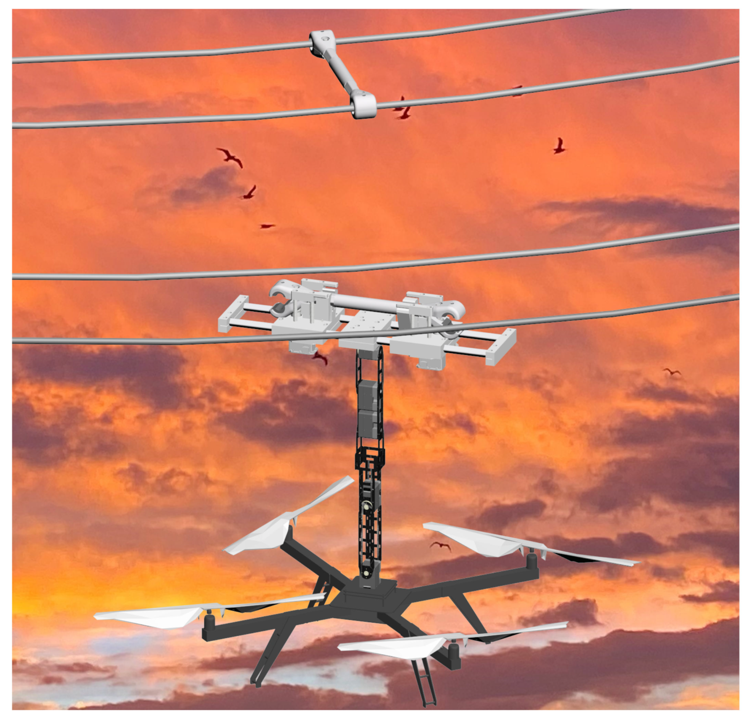
To minimize the risk to personnel performing various maintenance and repair tasks in such infrastructures, one idea is to develop advanced autonomous robotic systems that can replace humans. Due to the physical characteristics of such systems, aerial robotic manipulators could provide an ideal solution to the above problems [
5]. Due to the complexity of the tasks performed on power lines, practical robotic solutions that can handle this complexity require the combination of novel perception, manipulation, and control algorithms implemented in aerial robotic manipulator systems (
Figure 1).
The main objective of this paper is to analyze an electric spacer installation task, present a developed special end effector for this task, and control the motion of a robotic manipulator holding the end effector using a magnetic-field-based localization system developed for the fully autonomous installation of electric spacers on an in-phase parallel power line. Based on these objectives, the contributions of this paper are:
Th mechanical design of an end effector for the autonomous installation of spacers between two wires for power lines.
A method for the autonomous installation of spacers with the proposed end effector using magnetic-field-based localization.
Existing robotic power line devices are primarily for maintenance and monitoring purposes, requiring manual attachments to the wire [
6,
7]. Attachment to the wire is accomplished by various mechanisms, ranging from parallelogram linkages [
8] to novel clamping devices [
9] and v-shaped two-point slots [
7,
10].
In our previous work [
11], we presented a charging station for power lines and a corresponding end effector designed to install the charging station on the line. In [
12,
13], the authors presented the mechanisms for the installation and removal of aircraft warning spheres on power lines.
Unlike the previously presented solutions, the end effector presented here is intended for use with two parallel power lines.
The idea of using localization based on magnetic field measurements has been implemented for unmanned aerial vehicles (UAVs) that perch on power lines to recharge and thus extend their mission duration [
14]. In [
15], the authors investigated how to compute the position and orientation of UAVs with a minimum number of only three 3-axis magnetometers in the vicinity of two parallel power lines. However, this is not feasible in the application studied due to the specific design of the end effector and the pattern required to position the sensors. The same approach was experimentally validated in our previous work [
16], together with the numerical localization method for two wires. In [
17], a deep learning neural network architecture for precise indoor magnetic localization was developed to demonstrate the potential of precise magnetic positioning using smartphone sensors alone. In [
17], the authors questioned the feasibility of indoor magnetic localization and concluded that the most effective localization occurs in close proximity (10 cm) to the magnetic field. The work in [
18] presented simultaneous indoor localization and mapping based on the electromagnetic field of a building’s power grid. In [
19], a robust electromagnetic sensing system for 6-DOF pose estimation was presented, which can be useful for indoor localization and UAV landing scenarios, especially under challenging conditions. Considering some other application areas (e.g., medical), magnetic positioning technology is a suitable method for capsule localization in endoscopy [
20]. Considering logistics systems and, in particular, automated warehouses, magnetic positioning can serve well as a guidance method for automated guided vehicles (AGVs) [
21].
As for the work related to autonomous object handling, the basics of visual servoing are presented in [
22]. Park et al. [
23] designed a system that enables image-based visual servoing without prior depth information. The center of the target object is localized at the principal point of a camera. Using iterative lateral motion and one monocular camera, depth can be estimated. This paper shows that, with estimated depth and image-based visual servoing, it is possible to grasp an object. Gong et al. [
24] presented a projective homography-based uncalibrated visual servo approach. This presented approach is capable of both static positioning and dynamic tracking tasks for systems with unknown intrinsic camera parameters and eye-hand relationships. In [
25], a 3D electromagnetic motion control servo system with magnetic flux density feedback was developed for operation in non-line-of-sight environments. Such a system demonstrates the ability to control complex engineering systems based on magnetic field measurements. In [
26], an endoscope with a magnetically anchored and guided system (MAGS) for minimally invasive surgery was presented. In [
27], the visual-servo-based automatic tracking of a MAGS soft-body endoscope was achieved for the first time. In this case, a convolutional neural network (CNN) was used as a continuous visual servo controller. Such CNNs use only the reference image of the object and the current image of the camera to regress the control signal for the robot manipulator. To the best of our knowledge, this is the first paper in the field that deals with autonomous electrical spacer installation based on a special end effector and magnetic localization with a robotic manipulator. Moreover, the novel result is reinforced by the fact that this is the first autonomous installation of the device on power lines using magnetic localization.
The present paper is divided into six sections.
Section 2 describes the design of the dedicated tool for the automated installation of electric spacers.
Section 3 contains a problem definition, describes robot manipulator control modes, and presents a state machine for autonomous electrical spacer installation.
Section 4 presents a method for the magnetic localization of power lines based on magnetic field measurements.
Section 5 presents the hardware used and the experiments we performed to verify our method. In
Section 6, we present lessons learned and system limitations.
Section 7 summarizes the findings and results obtained.
2. End Effector for Spacer Installation
In this section, we present electrical spacer and specialized end effector designs for autonomous spacer installation.
2.1. Electrical Spacer
An electrical spacer is a mechanical device that keeps two, three, or four power lines at a constant distance from each other. Its purpose is to prevent short-circuiting between power lines and to dampen power line vibrations under harsh weather conditions. There are various designs of electrical spacers produced by different manufacturers.
This paper deals with the autonomous installation of electrical spacers for two wires shown in
Figure 2. It consists of a spacer body, two bolts with rubber dampers, and two lower jaw parts. The bolt clamps the conductor between the spacer body and the jaws on each side. From
Figure 2, it can be seen that when the spacer is open, the spacer jaws are free to move in all directions around the bolt that holds them.
The selected spacer is designed for manual installation by the maintenance crew. The procedure for manually installing the electrical spacers is to position the conductor between the jaws and the spacer body, then tighten the bolts by hand while adjusting the position and orientation of the jaws with the other hand. The same procedure is repeated on the other side of the spacer. This type of electrical spacer is manufactured for different distances between conductors, ranging from 300 to 600 mm. Such electrical spacers are not adaptable to different distances but are rather manufactured for certain predefined distance.
2.2. Design of the End Effector
The special end effector is designed for autonomous installation based on the construction of the electrical spacer. The design of the end effector for the installation of electrical spacers must adapt to the requirements defined by the design of the spacer, namely:
Keeping the spacer jaws open prior to installation;
Tightening the bolt;
Releasing the spacer when the installation is finished;
Providing adaptability for spacers of different lengths.
There is another requirement that the end effector must adapt to. According to the specification for the robot arm, the end effector must comply with a weight limit of 5 kg total weight, including the electrical spacer. The heaviest mass of the electric spacer predicted in this work is 1.5 kg. Thus, the mass of the end effector must be less than the limit of 3.5 kg.
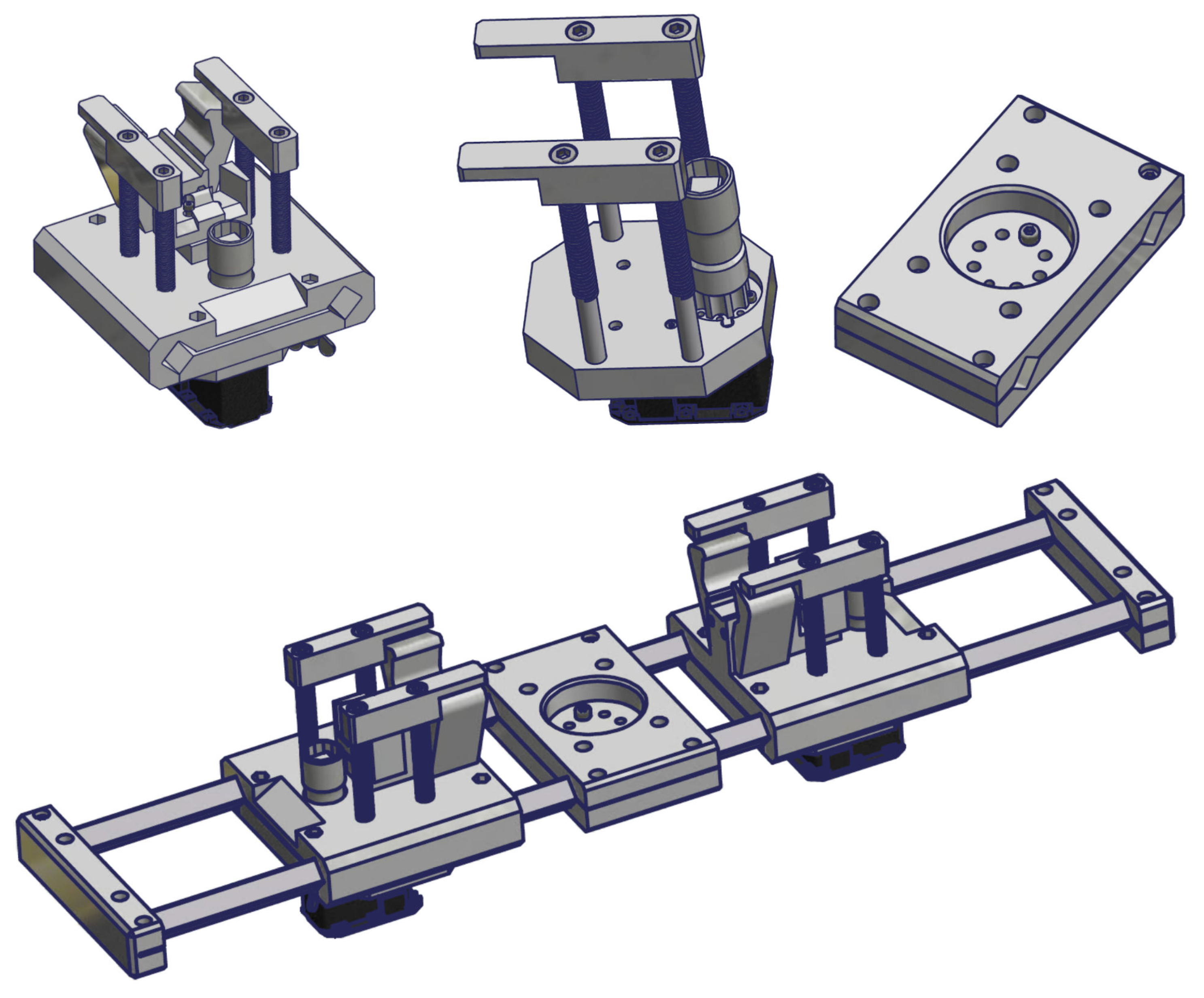
Each of these points is addressed by the design of the newly developed end effector. Its model and model components are shown in
Figure 3.
To accommodate the varying lengths of the spacer, the end effector is divided into three distinct subassemblies (see
Figure 3). Two subassemblies are identical and are designed to operate the opposite sides of the spacer, while the third subassembly of the end effector is designed to be positioned between these two identical subassemblies and is prepared for installation on the robot arm flange. All three subassemblies are designed to run on two guides that hold all three parts as a whole. Each of these subassemblies can be fixed at any point on the guides, so that the spacers of different length can be installed.
Prior to installation, the spacer jaws must be held open (see
Figure 2) to allow the spacer to enclose the conductors of the power line. This is achieved by holding the initial part of the jaws pressed with a spring (see
Figure 4).
The bolts are tightened by an electric motor mounted on the bottom of the end effector. The electric motor is mounted on the movable plate, which is connected to the rest of the end effector by a shaft holding the bolt tool and four rods with springs on the top of the end effector (see
Figure 4). These springs push the plate towards the rest of the end effector with a certain amount of force. This force ensures that the shaft with the bolt tool is pressed onto the bolt as the bolt is tightened. Since the upper part of the spacer is fixed in the end effector, the jaws start to close when the bolt is tightened, and the bolt moves towards the fixed part of the spacer.
To hold the electrical spacer in the end effector, there are two holders on each side that hold the spacer while it is transported to the installation site. The two holders on each side are connected by a spring that ensures they are closed when in an idle state. During transport, the holders are additionally locked by a lever mounted on the rods of the motor plate (see
Figure 4). In this way, they cannot be opened accidentally during the transport phase. When the spacer bolts are tightened, the rods and the lever are moved upwards, and in an instant, the lever moves above the level of the holder so that the holders can open. In this way, the holders are unlocked when the spacer is installed on the power line, and the end effector can be removed from the spacer.
The design process for such a compact, smart product in the form of a specialized end effector must be carried out in several iterative steps. In these steps, the number of actuators, the shape of the parts, and the mass of the parts are optimized. In the functional analysis, 14 functions are identified that require a force source for the movement:
Increasing/decreasing the distance between opposing operating side subassemblies;
Locking/unlocking the operating side subassembly position;
Gripping/releasing the electrical spacer;
Locking/unlock the electrical spacer;
Opening/closing the electrical spacer jaw (releasing/tightening the spacer bolt);
Moving the bolt tool on the bolt head along the bolt axis in both directions;
Keeping/releasinh the electrical spacer jaw in the open position.
Optimization was provided using the designers’ xperiences upgraded on theoretical backgrounds. The optimization focuses on the versatile use of the force sources and the shape of the subassembly parts. Some of these functions are performed manually on the ground.
2.2.1. Position of the Subassembly on the Guides
The side operating subassembly (see
Figure 5) is locked onto the guides by the frictional force caused by two screws that tighten the clamp (lower part). The hexagonal bolt in the hexagonal hole and the wing nuts allow tightening and loosening without additional tools (see
Figure 5). The clearance between the upper part and the guides allows the movement of the side operating subassembly along the guides when the screws are loosened. When the screws are tightened, the clamp pushes the guides to the upper part, and the position is fixed.
2.2.2. Holding and Locking the Spacer in the End Effector
The spring is used to create a minimal force that closes the electrical spacer holders. Opening and closing of the holder is accomplished by rotating the holder about a z-axis, as shown in
Figure 6. Gripping the electric spacer is done manually on the ground, which means that the in-air autonomous release of the electrical spacer is more critical. During the release, the electrical spacer is connected to the power lines, and the power line is used as the reaction force source, while the robot arm is used as the active force source in the vertical downward direction. This implies that the active force holding the electrical spacer in the end effector must be as small as possible. Minimizing this force is achieved by:
Taking advantage of the shape of the electric spacers;
Using two oppositely directed holders;
Optimizing the position of the axis of rotation of the holder;
Optimizing the shape of the holder.
The electric spacer holders are positioned on the hexagonal shape near the spacer jaw. When the upper force on the holder is vertical, its position leads to the opening of the holder. At this moment, the spring force is as low as possible, and the action and reaction force is also as low as possible. At the second moment, while the spring force is slowly increasing, the upper force on the holder changes its direction. At this moment, most of the normal force is absorbed by the solid body of the electric spacer, while the action and reaction force sources absorb most of the much smaller frictional force. The position of the electrical spacer must be fixed in the end effector while the robot arm is moving. While the robot arm is moving, the spacer jaws must remain open prior to installation. The electrical spacer can be unlocked from the end effector when the electrical spacer is installed on the power line. The electrical spacer is installed when the jaws are closed (the bolt is tightened and the bolt head is in the up position), and the conductor passes through the clamping jaws. The same force can be used for all functions:
The hexagonal shape of the electrical spacer and holders all around it stabilize its position. The extended tightening mechanism yoke allows the position of the spacer to be locked when the end effector is in the air and unlocked when the end effector is on the ground or the electrical spacer is installed.
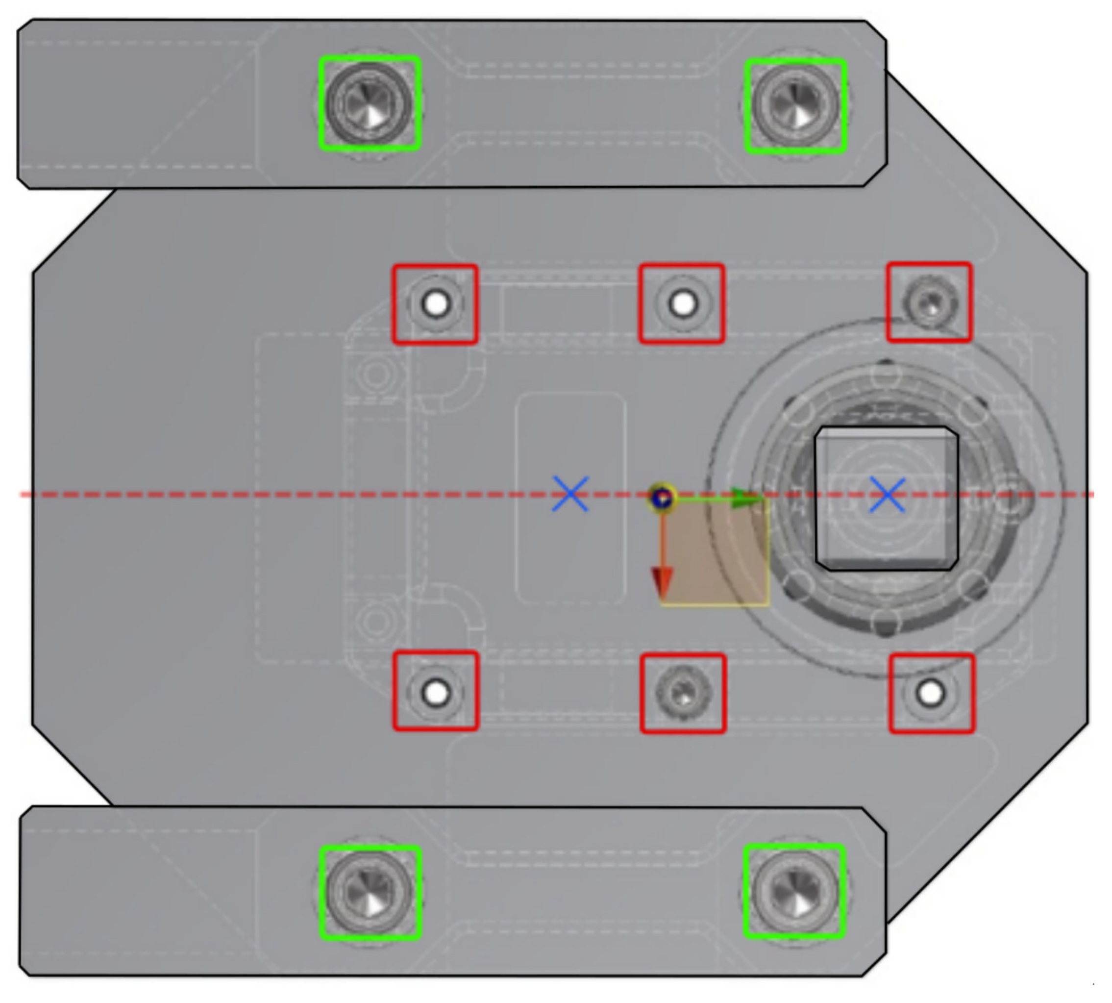
2.2.3. Closing the Electrical Spacer
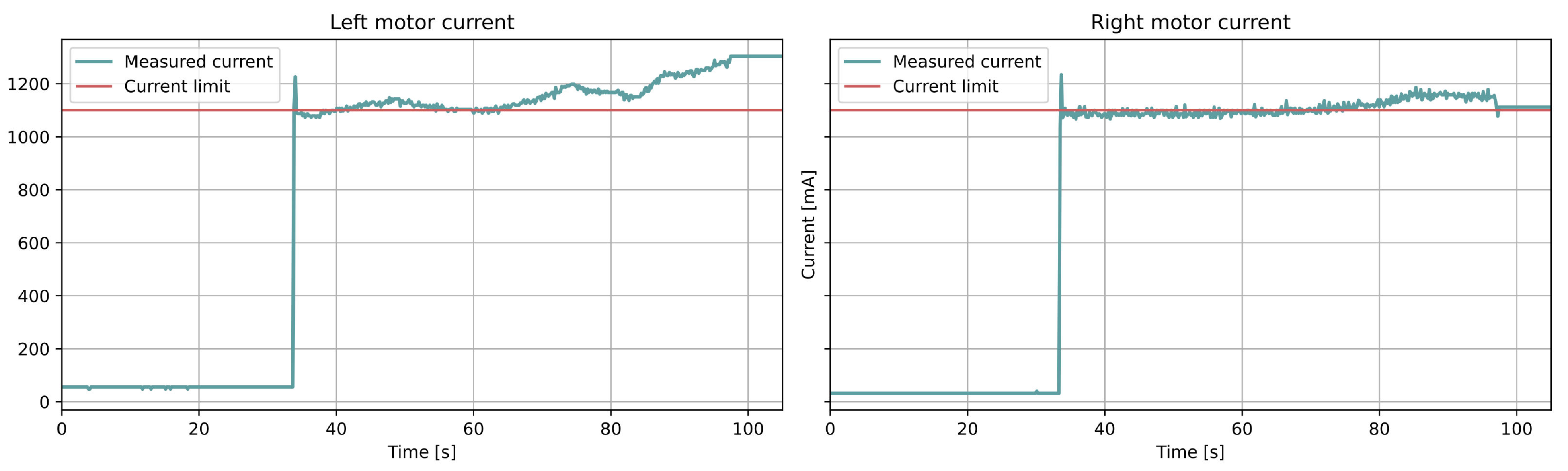
Closing the electrical spacer jaw (screw bolt) is the main function of the special end effector that has been developed. This function is performed by rotating the spacer bolt around its axis until the target torque is reached (the target torque is determined empirically by measuring the motor current and finding the current limit, which corresponds to the torque reached when the jaws are closed). The electric motor with the mounted bolt tool serves as the force source for opening and closing the jaws (tightening/releasing the spacer bolts). Tightening/releasing the spacer bolts leads to the movement of the bolt head along the bolt axis, which the bolt tool must follow. Opening the electrical spacer jaw (releasing the spacer bolt) pushes the bolt tool down. Contact between the bolt tool and the spacer bolts must be ensured when the electrical spacer jaw is closing. The movement of the electric motor and the bolt tool must be guided. Round tubes guided by holes in the main support part of the side operating subassembly are used to ensure this guidance. Four springs around those tubes supported with the main supportive part on one end and tightening mechanism yokes on the other end are used to ensure contact between the bolt tool and the spacer bolt. The tightening mechanism yokes are connected with long bolts through tubes to the support part of the electric motor. The electric motor with the bolt tool is attached to the support part with six bolts. All together, this comprises the tightening mechanism that moves along the axis of the spacer bolt axis while opening/closing the spacer jaws.
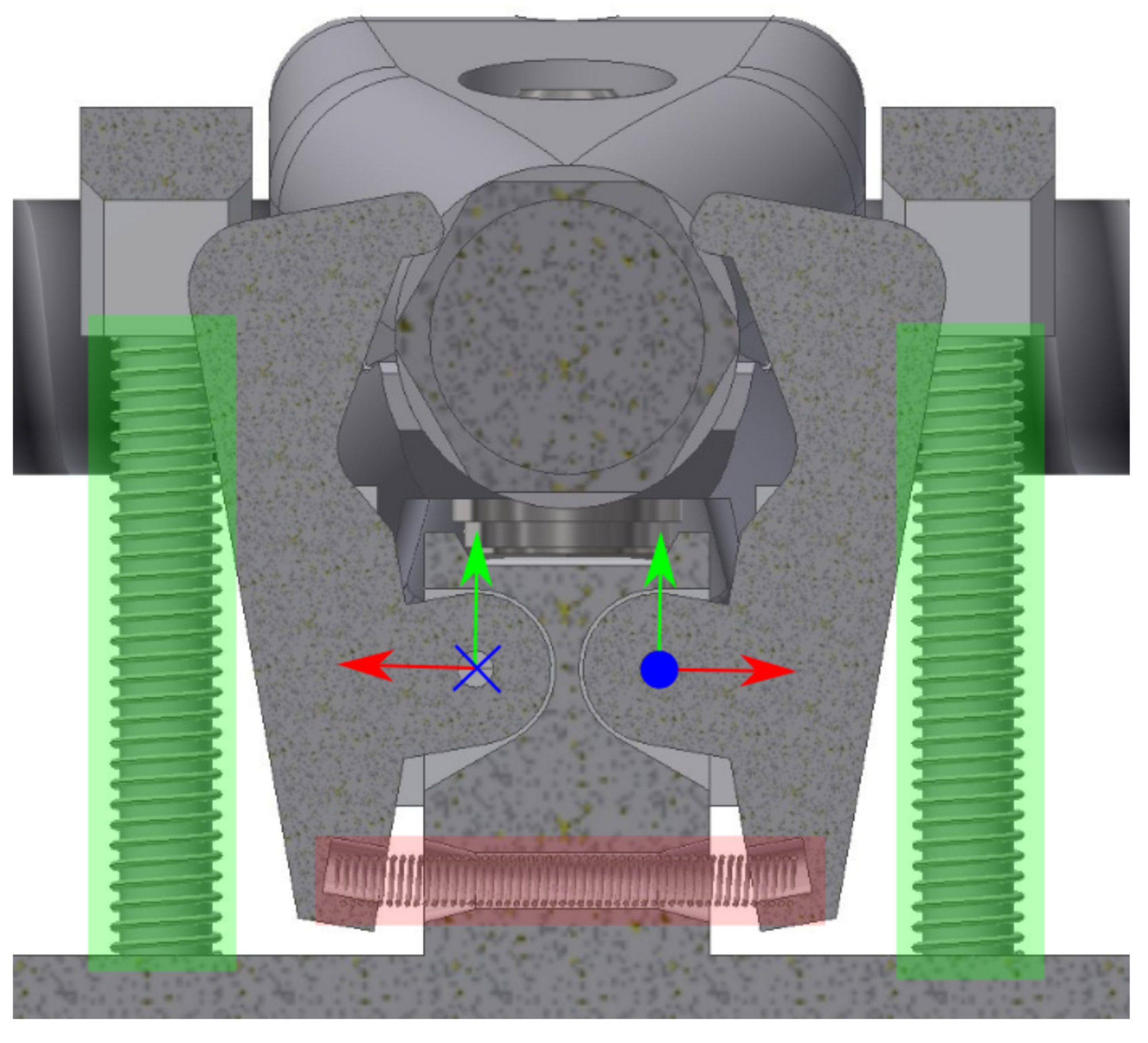
The critical point of the tightening mechanism design is the guidance. The mechanism is symmetrical with respect to the electrical spacer (red dashed line in
Figure 7), but optimization is required to minimize rotation about the perpendicular axis on the electrical spacer and increase the frictional force of the guidance.
There are three forces that must be considered: the resultant action force of the springs, the passive gravity force of the mass, and the reaction force of the spacer bolt on the bolt tool (see
Figure 7). With shape optimization, the position of the gravity force (center of mass without springs) and the position of the resultant force of the springs (corresponding to the center of mass of the springs) are approximated as much as possible. These two force components result in a minimal frictional force when guiding the bolt tool. When the electrical spacer jaw is closed (spacer bolt up), the spring force must be as small as possible. This results in minimal reaction force on the bolt tool as well as minimal friction force during its guidance. The torque of the electric motor is used to tighten the bolt. When the electrical spacer jaw is open (spacer bolts are in the lower position), the spring force slowly increases. As the spring force increases, the reaction force on the bolt tool and the frictional force for bolt tool guidance also increase. The electric motor is able to overcome the reaction and friction force, and the tightening mechanism moves and works as expected. The whole system works only if the jaws of the electrical spacer are in the open position until the electrical spacer is installed on the power lines. It is possible to evaulate the installation procedure phase (installed/not installed) based on the value of the current measurement of the electric motors used whilst tightening the bolt of the tightening mechanism.
2.2.4. Keeping Electrical Spacer Jaw in the Open Position
The electrical spacer and the spacer jaw have slots that allow the jaws to be held in the open position by the operator’s thumb during manual installation (see
Figure 8). In the special end effector described in this paper, the operator’s thumb force is replaced by the force of two springs. This force must be as small as possible so that it does not effect the tightening mechanism, the guidance, the friction force, or the spacer bolt axial force. In order to prevent an effect from an accidental lateral force on the electrical spacer jaw, the thumb replacement part has a limiter on each side and an optimized multi-purpose shape. The optimization of the spring force and interactive force position renders negative effects on the guidance of the tightening mechanism negligible.
The shapes of the multi-purpose parts and the multi-purpose force sources are achieved through multiple iterations of the optimization process. The result is our special end effector for the autonomous installation of electrical spacers that can be easily fabricated and functions properly. This approach, combined with weight requirements, makes additive technology the best choice for manufacturing most parts. Additive technology, when used in production, requires modeled mechanical component tolerances. The end effector mechanisms produced by additive technology, where different parts interact, require continuous optimization of part tolerances during product design to function properly. All these processes are successfully performed and presented in this work.
2.3. Prototype
The fabricated prototype is shown in
Figure 9. Due to its multipurpose shape and weight limit, most of its parts are 3D printed using polylactic acid (PLA) material. Its guide elements (square and round tubes) are AlMgSi0, its five springs are WNr1.1200, and its standard screws are zinc-galvanized. The actuators used for actuating the end effector are Dynamixel MX64 (basic parameters of Dynamixel MX64 are presented in
Table 1).
The whole production and assembly of the presented prototype of a specialized end effector for autonomous electrical spacer installation is carried out by additive technology (3D printing) and hand tools. The achieved weight of the prototype is approximately 2.3 kg, which is less than 2/3 of the target weight limit of 3.5 kg.
The end effector is designed to approach the power lines from below, and when it reaches the desired height, it is rotated so that the spacer surrounds the lines on both sides. The actuators tighten the bolt to close the jaws of the spacer. When the spacer closes on the conductor, the end effector is unlocked from the spacer and can be removed by pulling it downwards.
Figure 10 shows the procedure for installing the electrical spacers on power lines.
3. Robot Control Problem Statement
From a control perspective, the procedure for installing the spacer is divided into three tasks, which are carried out sequentially in three logical steps. Since the end effector must approach the wires from below, the first step is to position the end effector with the spacer in the approach pose, i.e., below the wires. The second step involves servoing based on magnetic-field-based localization towards the preinstallation pose, which is defined by the spacer being positioned between, at the same height as, and almost parallel to the wires. The third step involves rotating the spacer (end effector) so that the jaws of the spacer enclose the wires on both sides. This procedure is shown in
Figure 11. For the installation, we use a 6DOF robot arm Schunk LWA4p. A complete kinematic (forward, inverse) derivation of the robotic arm can be found in [
28].
3.1. Approach Pose
The first step consists of positioning the robot manipulator with the corresponding end effector in the approach pose, defined by:
where
,
, and
define the position of the approach pose and
,
,
, and
define the quaternion that represents the orientation of the approach pose. If we define two parallel conductors as two lines in 3D, they can be described by the following equations:
where
defines the points of a first line,
defines the points of a second line,
is one point on the first line,
is one point on the second line,
is a line direction vector common for both lines, and
and
are scalars. The origin of the approach pose is chosen based on the points on each conductor (defined as a line in Equation (
2)) closest to the robot base, i.e., the origin of the global coordinate frame
[
29]:
where
is the point on the first line closest to the origin of
and
is the point on the second line closest to the origin of
. The origin of the approach pose is calculated by:
where
o is the initial offset along the
z axis from the spacer to the wires and
is the distance along the
z axis from the last robot joint to the electrical spacer. The quaternion defined by
, and
is determined from
, taking into account the following assumptions:
This implies that the orientation of the power lines is defined only by a yaw angle:
where
is the yaw angle of the conductors. The yaw angle of the end effector is defined by:
where
is a small offset added to avoid positioning magnetometers parallel to the conductors. By simple conversion, the end effector yaw angle
can be transformed into the quaternion (
,
,
,
).
3.2. Preinstallation Pose
Starting from the approach pose, we use magnetic localization and servo control of the robot arm to position the end effector between the conductors in the preinstallation pose. The preinstallation pose is defined as follows:
where
The quaternion (, , , ) is determined from the desired yaw angle .
3.3. Installation Pose
After positioning the end effector in the preinstallation pose between the power lines, we must perform the necessary rotation of the tool to position the spacer vertically and drop the conductors between the jaws of the spacer, as shown in
Figure 10. This pose is called the installation pose, and it is defined as:
where the quaternion (
,
,
,
) is calculated from the desired yaw angle
.
Figure 11 shows, from left to right,
,
, and
in relation to the power lines.
The next step is to close the jaws of the spacer around the conductor by the actuators of the end effector. The spacer is considered closed and the actuator is stopped when its current rises above a certain threshold value for a certain amount of time:
where
is the actuator current and
is the current limit at which the spacer is considered closed.
3.4. Motion Planning and Trajectory Execution
For motion planning and trajectory execution, we use MoveIt! [
30]
https://moveit.ros.org/ (accessed on 11 February 2023), developed by:
https://picknik.ai/ (accessed on 11 February 2023), ROS
https://www.ros.org/ (accessed on 11 February 2023), and Gazebo
http://gazebosim.org/ (accessed on 11 February 2023) to safely plan a collision-free path of motion. We use OMPL [
31] as a motion planning library and Rapidly Exploring Random Trees (RRT) as part of MoveIt! for planning. We added an end effector model in URDF and power lines to the planning scene to enable the collision-free execution of the trajectory.
3.5. Robot Arm Servoing
After reaching the approach pose, the servo control of the robot arm is used to reach the preinstallation pose. The servo control of the robot arm is realized with four P-controllers and the MoveIt! servo ROS package.
The difference between the current pose of the end effector and the preinstallation pose, which is calculated based on the current estimation of the power line position, is used as an input signal for the P-controllers.Three P controllers are used to track the end effector’s position (see Equations (
11)–(
13), while one P controller is used to track the end effector’s orientation (see Equations (
14)–(
18)). The output of each P controller depends on the gains (
,
,
) and the error, which is calculated as the difference of the commanded value for each axis (
,
,
) and the measured end effector pose (
,
,
) for each axis.
while one P controller is used to control the end effector orientation. The orientation error is determined as the product between the desired orientation quaternion
and the inverse quaternion of the current end effector orientation
[
32],
The orientation error quaternion is converted into an axis
and an angle
representation. Using this angle and the P controller, the angle magnitude is computed as follows:
Using the calculated axis, we can calculate angular velocity for the end effector, as follows:
The first three P controllers are used to generate the control input to reach the desired end effector position, as shown in Equations (
11)–(
13). We assume that the magnetic estimation will be correct enough that the commanded position will not lead the system to instability; furthermore, we set
in order to slow down the continuous arm movement to the commanded position. We experimentally evaluated that adding a
or
component to the control loop for robot arm servoing leads to the degraded performance of the controller.
The fourth P controller controls the magnitude of orientation error, as shown in Equation (
15). The magnitude of the orientation angle error is used to calculate angular velocity for each end effector axis, as shown in Equations (
16)–(
18). The outputs of the four P controllers with gains
,
,
, and
determine the velocity of the end effector in the task space. Robotic arm servoing is implemented using the Jacobian pseudoinverse, as shown in [
30]. Robot arm servoing control structure can be seen in
Figure 12.
We try to exploit the fact that the magnetic field measured by the magnetometers is stronger the closer the end effector is to the power lines. Therefore, the localization becomes more accurate and precise as the error between the tracked pose and the current pose of the end effector decreases.
3.6. State Machine
We have developed a finite state machine that divides the process of installing the electrical spacer on power lines into logical states that are also the sequential tasks of the entire process. The installation process is divided into two superstates and two final states. The superstates are called the stationary arm and the moving arm.
Each superstate contains multiple states. The moving arm superstate contains states that require robot arm movement, such as trajectory execution, servoing, and rotating the tool. The stationary arm superstate contains all states in which the robot arm is stationary, such as the initial pose, the approach pose (), the preinstallation pose (), the installation () pose reached, and the install spacer. In addition to superstates, we define two final states that correspond to successful and failed spacer installation tasks. The state transition from the initial pose to trajectory execution is triggered with a command that contains the pose , a timeout parameter , and the scalar distance . The robot reaches its approach pose if the distance function between the commanded and the measured end effector pose is smaller than the distance and if the current task execution time t is smaller than the timeout .
The distance function is defined as the sum of the Euclidean norm of the pose vector position components and the quaternion distance of the pose vector orientation components. The quaternion distance is defined as
where
presents the dot product between two quaternions. The distance function for the approach pose is defined in Equation (
19).
The rest of the state transitions and conditions can be inferred from
Figure 13, which shows a Harel statechart [
33] of the system.
Yellow rectangles depict superstates, white rectangles depict states, and red and green rectangles depict final states. The transitions between states are shown with arrows. Black text above a state transition arrow describes a command sent. A blue text above a state transition describes a condition that must be met for state transition. The state machine was implemented using smach_ros
http://wiki.ros.org/smach_ros (accessed on 10 February 2023) and ROS actionlib
http://wiki.ros.org/actionlib (accessed on 10 February 2023).
4. Localization of Power Lines
This section presents the numerical method for localization based on the magnetic field strength of two parallel straight conductors carrying the same current, similar to the one presented in [
16].
4.1. Magnetic Field around the Conductor
The magnetic field strength produced by the flow of current through a long, straight conductor is:
where
B is the strength of the magnetic field,
is the vacuum permeability,
r is the distance from the conductor, and
I is the conductor current.
Equation (
20) provides the magnetic field strength at a distance
r. The direction of the field is determined by the right-hand rule with respect to the conductor. Its vector always has a direction that is circumferential with respect to the isomagnetic lines.
The vector of the magnetic field
at a point
generated by two parallel conductors (defined as 3D lines by Equation (
2)) carrying the same current
I can be calculated by:
where
, the magnetic field vector generated by one line,
k, is:
where
is the point on the conductor
k closest to the point
, which can be calculated using Equation (
2), with
calculated in the following way:
4.2. Numerical Method for Locating Two Power Lines Based on Three or More Magnetometers
At least three magnetometers at different locations are needed to locate two conductors [
15]. Several assumptions have been made to avoid ambiguity and to increase the stability of the location determination:
- A-1
The conductors are parallel and at a distance from each other;
- A-2
The distance from a magnetometer to the nearer conductor is less than ;
- A-3
The current through the conductors will be less than ;
- A-4
The conductors are parallel to the ground;
- A-5
The robot is never directly above the conductors;
- A-6
Two magnetometers must not be parallel with the conductors.
Assumption A-1 is usually satisfied if there is no strong wind. The assumptions A-2 and A-3 can always be satisfied for sufficiently large and . The assumption A-4 will not necessarily be satisfied under realistic conditions, but its angle will always be relatively small. Since the spacers are set up from below, A-5 can be assumed. If the magnetometers are placed parallel to the conductors, they will measure the same values, so A-6 must be satisfied for successful localization.
The measurements of all magnetometers is measured in their frames defined by the vector and the rotation matrix (assuming the same orientation of all magnetometers) with respect to the global frame .
Under the assumption that both conductors are parallel to the ground, the direction of the conductors in
(vector
) for the setup with 3 magnetometers can be derived from the equation:
where
is the measurement of magnetometer
i expressed in the global coordinate frame:
A special case occurs when all magnetometers are in the same plane as the conductors when (
25) is a null vector. However, this problem can be solved by the careful choice of the relative position of the magnetometers, and it is sufficient if at least one magnetometer is not in the same plane as the conductors.
For the case of three magnetometers and two conductors, the location of the conductors can be determined by minimising the criteria:
where
is the location of magnetometer
i in the global frame (see
Figure 14).
The criterion (
26) is defined with 7 variables (3 in
, 3 in
, and
I). Since it was assumed that the conductors are parallel to the ground plane and to each other at a known distance, and that
and
are arbitrary conductor points defined by (
2), the number of variables can be reduced.
Two independent variables define
, but the vector perpendicular to
needs to be determined first:
where
is a vector perpendicular to the
and
z vectors. Now,
can be represented with variables:
where
and
are two scalar variables.
can be determined by:
Given the Equations (
22), (
23), (
28), and (
29), Equation (
26) becomes:
The problem comes down to the minimization of three variable criteria. This minimization can be carried out by various methods. Due to the constraint of
and
, the optimal triplet
,
, and
for criteria (
30) will be within the range
,
, and
, respectively. One way to find the optimal solution would be to discretize these ranges with the steps
,
, and
, respectively, and go through all combinations of triplets
. After finding the triplet with the smallest criterion, further refinement around the triplet with the smallest criterion can be performed with steps
,
, and
.
4.3. Processing the Measurements of the Alternating Magnetic Field
The first step in magnetic localization is processing the raw data collected by the magnetometers. Magnetometers measure magnetic fields, which are affected by various sources, such as the earth’s magnetic field, the electric field of the power lines, noise from electric motors, etc. Since power lines generate an alternating magnetic field of known frequency (50 or 60 Hz), the first step is to estimate the amplitude and phase in the x, y, and z directions of this field, which defines the influence of the power line. This information is then used in the further course of the localization procedure to determine the location of the power lines.
The measured magnetic field can be estimated with:
where
is an alternating magnetic field,
D is a DC component,
A is the signal amplitude,
f is a frequency of the signal (usually 50 or 60 Hz),
is its phase offset, and
t is the time instance.
In our previous work [
29], the method of extracting the amplitude and phase of the measured magnetometer signal is presented. The method is based on discrete Fourier transformation and has been shown to work at a frequency of 1 Hz and with a large number of samples. To increase the frequency of the system, an improved processing system based on numerical optimization is developed. This system is computationally more demanding but requires a smaller number of samples to determine
A,
D, and
. The criterion used for optimization is [
16]:
where
is the ith of
N samples used for processing and
is the sampling time. The optimization is performed using the Nelder–Mead optimization algorithm, which is run twice for two different initial parameter sets
for optimization (see
Table 2).
The same optimization procedure is repeated for all three magnetometers used for each of the x, y, and z axes. If the phases of two axes coincide, they have the same direction, and if their phases are apart by radians, they have the opposite direction. For this purpose, all measurements must be synchronized.


