Loss Analysis of a Transonic Rotor with a Differential Approach to Entropy Generation

Abstract

The loss mechanism of transonic axial compressors is a long-standing problem that involves almost all types of entropy generation in fluid flows, such as skin friction, shock waves, shear flows, corner separation, and tip vortices. Primarily, sources need to be identified and quantitative comparisons of their contributions need to be made. For such determination, we propose herein a differential approach to entropy generation, called the “differential approach”. Two case studies are analyzed to determine the applicability of this approach: (1) laminar and turbulent incompressible flows in straight circular ducts and (2) turbulent compressible flows in convergent-and-divergent nozzles with shock waves. The results lead to the following conclusions: (a) Qualitatively, the differential approach works well, and the quantified measure is reliable if it is calculated with quality meshes and a suitable turbulence model. This means that the differential approach can be a good tool for predesign optimization. (b) When shocks occur within flow fields, the shock-induced boundary-layer separation can generate more loss than the shock loss alone. Subsequently, the differential approach is applied to complex flows in the NASA Rotor 67, which is a well-known bench-test transonic rotor. The results show that the differential approach not only determines the local losses and associates the source of losses with the flow structures but also qualitatively compares and identifies the largest contributors. These results provide a theoretical foundation for optimizing rotor design and enhancing stability.

1. Introduction

1.1. Review of Differential Entropy Generation

Entropy generation is one of the common measures of irreversibility in fluid devices. Bejan [1] proposed the blending of the first and the second laws of thermodynamics with fluid dynamics and heat transfer in an integral form to minimize entropy generation in thermal systems, such as cryogenics, a smooth tube with heated or cooled solid surface, or solar power plants, and obtained the following equation:

$$\dot{W}=-{\displaystyle \frac{d}{dt}}\left(E-T_{0}S\right)+{{\displaystyle \sum }}_{i=1}^n\left(1-{\displaystyle \frac{T_0}{T_i}}\right){\dot{Q}}_i+{{\displaystyle \sum }}_{in}\dot{m}\left(h^{\circ }-T_{0}s\right)-{{\displaystyle \sum }}_{out}\dot{m}\left(h^{\circ }-T_{0}s\right)-T_0{\dot{S}}_{gen}$$

(1)

In Equation (1), if the reversible work equates to zero entropy generation ($\dot{S_{\mathit{gen}}}$), then

$${\dot{W}}_{rev}-\dot{W}=T_0{\dot{S}}_{gen}.$$

(2)

Except for the time-dependent term, all quantities in Equations (1) and (2) are the mean values applied to or obtained from the surface of the systems under consideration.

Bejan’s idea is of strategic value and can be expanded to many areas of thermal engineering, some of which are reviewed in Ref. [1]. To directly integrate fluid dynamics into Equation (2), the solutions are naturally sought directly from the governing equations of fluid flow, which are the equations of mass, momentum, and energy conservation laws. The second law of thermodynamics is also derived from these conservation laws, so entropy generation needs to be calculated by post-processing after the fluid flow and heat transfer are determined by applying these conservation laws.

About 20 years ago, Herwig et al. [2,3,4,5,6] studied extensively a differential entropy-generation approach. Although this idea was not new [7], they extensively studied the associated computation in conjunction with turbulence models in a computational fluid dynamics (CFD) environment. A brief review [5] is given below for convenience. The three conservation laws are

$$\frac{\partial \rho }{\partial t}+\frac{\partial \left(\rho u_i\right)}{\partial x_i}=0,$$

(3)

$$\frac{\partial \left(\rho u_i\right)}{\partial t}+\frac{\partial \left(\rho u_j{u}_i\right)}{\partial x_j}=-\frac{\partial p}{\partial x_i}+\frac{\partial {\tau }_{ji}}{\partial x_j}+\rho f_i,$$

(4)

$$\frac{\partial \left(\rho e_t\right)}{\partial t}+\frac{\partial \left(\rho u_i{h}_t\right)}{\partial x_i}=\frac{\partial }{\partial x_i}\left(\lambda \frac{\partial \theta }{\partial x_i}\right)+\frac{\partial }{\partial x_j}\left({\tau }_{ji}\cdot u_i\right),$$

(5)

where subscript t denotes the total quantity, i.e.,

$$e_t=e+\frac{1}{2}\left(u_i{}^2-v_i{}^2\right); h_t=e+\frac{p}{\rho }+\frac{1}{2}\left(u_i{}^2-v_i{}^2\right),$$

(6)

Multiplying Equation (4) by $u_i$ yields the transport equation of kinetic energy that, after substitution into Equation (5), becomes the following transport equation of static enthalpy:

$$\frac{\partial \left(\rho h\right)}{\partial t}+\frac{\partial \left(\rho u_{i}h\right)}{\partial x_i}=\frac{dp}{dt}+\frac{\partial }{\partial x_i}\left(\lambda \frac{\partial \theta }{\partial x_i}\right)+{\tau }_{ji}\frac{\partial u_i}{\partial x_j},$$

(7)

The transport equation of entropy may be obtained by applying the thermodynamic relation of properties $Tds=dh-\frac{1}{\rho }dp$, which gives

$$\rho \frac{ds}{dt}=\frac{\partial \left(\rho s\right)}{\partial t}+\frac{\partial \left(\rho u_{i}s\right)}{\partial x_i}=\frac{\partial }{\partial x_i}\left(\frac{\lambda }{\theta }\frac{\partial \theta }{\partial x_i}\right)+\frac{\lambda }{{\theta }^2}\frac{\partial \theta }{\partial x_i}\frac{\partial \theta }{\partial x_i}+\frac{2\mu {\epsilon }_{ij}{s}_{ij}}{T},$$

(8)

The last two terms in Equation (8) are always positive and are called the thermal entropy generation rate (EGR) ${\dot{S}}_C^{‴}\equiv \frac{\lambda }{{\theta }^2}\frac{\partial \theta }{\partial x_i}\frac{\partial \theta }{\partial x_i}$, which stems from the finite temperature gradient, and viscous EGR ${\dot{S}}_D^{‴}\equiv \frac{2\mu {\epsilon }_{ij}{\epsilon }_{ij}}{T}$, which stems from the friction caused by viscosity. Entropy generation due to heat transfer can be identified by using

$$\frac{1}{\theta }\frac{\partial }{\partial x_i}\left(\lambda \frac{\partial \theta }{\partial x_i}\right)=\frac{\partial }{\partial x_i}\left(\frac{\lambda }{\theta }\frac{\partial \theta }{\partial x_i}\right)+\frac{\lambda }{{\theta }^2}\frac{\partial \theta }{\partial x_i}\frac{\partial \theta }{\partial x_i},$$

(9)

The above equations are exact when applied to direct Navier–Stokes simulations. When conducting Reynolds-averaged Navier–Stokes (RANS) simulations, the flow is divided into the mean flow plus its fluctuation counterpart, so entropy generation takes the forms:

$${\dot{S}}_D^{‴}=\frac{2\mu {\overline{\epsilon }}_{ij}{\overline{\epsilon }}_{ij}}{\overline{\theta }}+\frac{2\mu \overline{\epsilon {\prime }_{ij}\epsilon {\prime }_{ij}}}{\overline{\theta }},$$

(10)

$${\dot{S}}_C^{‴}=\frac{\lambda }{{\overline{\theta }}^2}\frac{\partial \overline{\theta }}{\partial x_i}\frac{\partial \overline{\theta }}{\partial x_i}+\frac{\lambda }{{\overline{\theta }}^2}\overline{\frac{\partial \theta \prime }{\partial x_i}\frac{\partial \theta \prime }{\partial x_i}},$$

(11)

For incompressible and compressible flows in a Cartesian coordinate system, the equations take the form

$${\dot{S}}_{irr,\overline{D}}^{‴}=\frac{\mu }{T}\left(2\left[{\left(\frac{\partial \overline{u}}{\partial x}\right)}^2+{\left(\frac{\partial \overline{v}}{\partial y}\right)}^2+{\left(\frac{\partial \overline{w}}{\partial z}\right)}^2\right]+{\left(\frac{\partial \overline{u}}{\partial y}+\frac{\partial \overline{v}}{\partial x}\right)}^2+{\left(\frac{\partial \overline{u}}{\partial z}+\frac{\partial \overline{w}}{\partial x}\right)}^2+{\left(\frac{\partial \overline{v}}{\partial z}+\frac{\partial \overline{w}}{\partial y}\right)}^2\right),$$

(12)

$${\dot{S}}_{irr,D\prime }^{‴}=\frac{\mu }{T}\left(2\left[\overline{{\left(\frac{\partial u^{\prime }}{\partial x}\right)}^2}+\overline{{\left(\frac{\partial v^{\prime }}{\partial y}\right)}^2}+\overline{{\left(\frac{\partial w^{\prime }}{\partial z}\right)}^2}\right]+\overline{{\left(\frac{\partial u^{\prime }}{\partial y}+\frac{\partial v^{\prime }}{\partial x}\right)}^2}+\overline{{\left(\frac{\partial u^{\prime }}{\partial z}+\frac{\partial w^{\prime }}{\partial x}\right)}^2}+\overline{{\left(\frac{\partial v^{\prime }}{\partial z}+\frac{\partial w^{\prime }}{\partial y}\right)}^2}\right),$$

(13)

$${\dot{S}}_{PRO,\overline{C}}=\left(\frac{{\overline{\Phi }}_{\theta }}{T^2}\right)=\frac{\lambda }{{\overline{T}}^2}\left[{\left(\frac{\partial \overline{T}}{\partial x}\right)}^2+{\left(\frac{\partial \overline{T}}{\partial y}\right)}^2+{\left(\frac{\partial \overline{T}}{\partial z}\right)}^2\right],$$

(14)

$${\dot{S}}_{PRO,C\prime }=\frac{{\alpha }_t}{\alpha }\frac{\lambda }{{\overline{T}}^2}\left[{\left(\frac{\partial \overline{T}}{\partial x}\right)}^2+{\left(\frac{\partial \overline{T}}{\partial y}\right)}^2+{\left(\frac{\partial \overline{T}}{\partial z}\right)}^2\right],$$

(15)

Although in early trials Kock and Herwig [2] proposed a specially designed wall function to incorporate in the k–ε turbulence model, Herwig et al. [3] later argued that the k–ω shear stress transport model is a better choice with a proper grid density in the flow field. They recommend the following equation:

$$S_{irr,D\prime }^{‴}={\beta }^{*}\frac{\rho \omega k}{T_m},$$

(16)

where ${\beta }^{*}=0.09$, $\omega$ is the characteristic frequency, and k is the kinetic energy of the turbulent fluctuations. The special wall function is no longer required.

1.2. Research into Loss in Turbomachinery

The common parameters used as loss indicators include entropy and total pressure ratio, both of which are indirectly related to entropy generation. Entropy is a state property, which by definition cannot be used as a loss indicator. However, the entropy change across a control volume in an adiabatic process equals the entropy generation within the control volume, which can be used to measure loss. Therefore, the entropy contours are sometimes regarded to show the “loss distribution” because the more entropy generated through the adiabatic process, the more entropy accumulates at the outlet. However, this interpretation of entropy contours may be misleading and should be applied with caution.

The total pressure loss coefficient is an integrated approach for obtaining the loss indicator. It is the ratio of total outlet pressure to the total inlet pressure for the control volume under study. It is related to entropy generation based on the following thermodynamic relation:

$$\mathsf{∆}s=C_{p}ln\left({\displaystyle \frac{T_{t2}}{T_{t1}}}\right)-Rln\left({\displaystyle \frac{P_{t2}}{P_{t1}}}\right).$$

When the process is adiabatic, the total temperature is constant. Thus, the total pressure ratio equals the entropy change, which consequently is the entropy generation for the adiabatic process.

The above approaches both use the integral format because they rely on the adiabatic process within the control volume, so the details within the control volumes are averaged. The differential approach (i.e., Equations (10) and (11)) is used to identify loss sources. In its early days, the differential approach served mainly to analyze the loss during heat transfer [6] and to optimize the design of pipeline structures [3,4]. Recently, its application has been extended to turbomachinery [8,9,10,11,12,13,14,15].

References [8,9,10] apply the differential approach to study the loss mechanism in turbines. Denton and Pullan [8] studied a cascade and a low-speed turbine and RANS numerical simulation method was used. Although they used the differential approach, they presented their results in an integrated form by breaking down the entire computation domain into 12 subregions and listing the percent contributions to entropy generation from each subregion. Metodi et al. [9] used the differential approach to study the loss mechanism of hub and shroud sealing flows with RANS. They focused on the loss due to the purge flow–passage vortex interaction in the presence of passage secondary flow and tip clearance flow. Lin et al. [10] used a turbine cascade VKI LS89, which is the guide vane cascade of a generic transonic high-pressure turbine. With more than 20 M cells, the high-fidelity simulation (the Delayed Detached Eddy Simulation, or DDES) produces impressive contours of local entropy generation, with the contribution of wake vortices and shock waves clearly visible. Cascades are an ideal scenario for applying the differential approach [5,12,13]. Loss sources are the interaction in the corner between the blade suction surface and the hub, corner separation, and corner vortex in addition to the interaction between the corner and wake flows. Without localized entropy generation, the contribution of each loss source cannot be identified. Li et al. [13] used a hybrid RANS + Large Eddy Simulation (LES) model, called a shear stress transport detached eddy simulation, for the corner flow simulation, while Wang et al. [12] used a delayed detached eddy simulation. Both investigated the same cascade that was tested in Ecole Centrale Lyon [15]. The Mach number of the incoming flow in both studies was 0.117, so no shock waves were generated in the flow field.

A few studies have also reported the application of the differential approach to rotors. Zhang et al. [11] simulated the entropy generation under stall conditions in a centrifugal fan. They reported that entropy generation increases after stalling. Zhang et al. [14] analyzed the entropy generation of a mixed-flow compressor with casing treatment and investigated the flow structure of the tip leakage flow and flow separations near the rotor leading edge. Furthermore, they analyzed the loss mechanisms for cases with and without casing treatment and quantified integral losses in several regions. Although the design speed for this compressor was as high as 60,125 rpm, at which the flow at the tip of the compressor would be supersonic, the speed under study was only 30,000 rpm because the need for stall margin improvement was in this speed range. No shock waves occurred at this partial rotor speed.

1.3. Motivation for Present Research

The present study strives to identify the sources of loss within a transonic compressor rotor. Two research questions are posed: (1) Which turbulence model should be chosen? and (2) Can the chosen model handle the complexity of flow structures involving shocks and shock-induced separation?

The scope of this study is limited to RANS to avoid the significant computational cost of LES and its variants [16,17,18]. The literature shows that RANS can be used for flows in many fluid machines, including turbomachinery [19,20,21,22,23,24,25,26,27,28,29,30,31,32,33]. However, to explore the applicability of the differential approach with commercial CFD code, two cases are carefully selected and tested before extending the differential approach to a transonic rotor. First, a straight duct with smooth wall boundaries and various Reynolds numbers is chosen as a reference for its simple geometry and abundant features in fluid dynamics. When the Reynolds number is small and the flow is laminar, analytical solutions for the pressure drop can be obtained with isothermal boundary conditions. When the Reynolds number is large enough to ensure fully developed turbulent flow within the pipe, the ability to predict the pipe loss using the differential approach can be analyzed by applying the well-known Moody chart, which comprises the experimental data of the friction coefficient and has been widely used since 1944.

Second, a convergent-divergent nozzle named the “Laval nozzle” is designed to study the effect on losses of simple fluid compressibility. In particular, this approach focuses on the shock wave and its interaction with the boundary layer. The distinguishing feature of shock waves in the real world is that they are extremely thin, with thicknesses of the order of the mean free path of gas molecules [7]. With RANS, the shock wave thickness far exceeds a molecule’s mean free path. However, the results show that RANS can match the ratios of flow properties, such as Mach number and the static pressure ratio, across the shock wave via the one-dimensional (1D) shock wave theory. Surprisingly, the loss in the Laval nozzle is dominated by the shock-induced boundary-layer separation, which is much greater than the loss in the shock itself.

A high-speed axial compressor rotor is chosen to illustrate how the differential approach functions in complicated realistic engineering cases. The distribution of the volumetric EGR is plotted as colorized contours, similar to the state properties of fluids (e.g., pressure and temperature). However, precautions are taken in assigning physical meaning to such contours because entropy generation is a path-dependent quantity, whereas the fluid properties are path-independent. When the grid is drawn evenly and reasonably, the EGR distribution is consistent with that of entropy generation, which reflects the local loss, so it can be applied to various fluid structures or flow fields.

1.4. Structure of This Paper

This study uses ANSYS ICEM to generate structured meshes for three cases and ANSYS CFX for numerical simulation. This paper is organized as follows: Section 2 presents two case studies, both of which contain their descriptions of numerical models, followed by the presentation of the flow fields. The aim of case one is to obtain the total entropy generation related to the commonly used friction coefficient of straight pipes, which enables a direct comparison with the analytical solution and the experimental results (i.e., the Moody chart). Case two presents the flow fields in such a way that the Laval nozzle is simulated to investigate the application of the differential approach to a compressible flow field and the results of this approach to treating shock waves. Section 3 simulates the NASA Rotor 67 (R67), which is a well-known bench-test transonic rotor, with the RANS model. The differential approach is analyzed for complex flow structures such as tip vortex, leakage streamline, corner vortex flow, and wake, as well as interactions between these flow structures. Finally, Section 4 summarizes and concludes.

2. Case Studies

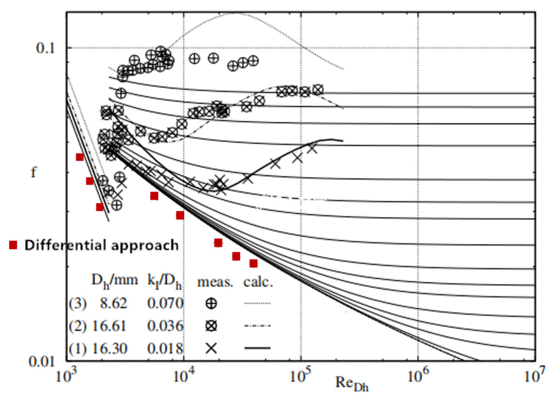
2.1. Case One: Laminar and Turbulent Incompressible Flows in Straight Circular Ducts

A small yet long circular duct with isothermal wall boundaries is chosen as the first test case. The fluid is water; so, the flow is incompressible. The exit pressure is fixed at 0.1013 MPa, and the inlet pressure is varied to obtain different types of flows inside the duct. For laminar flows, the length-to-diameter ratio is set to a very large number of 25,000 (500 m long and 0.02 m diameter) to ensure sufficient mass flow rate and pressure difference through the pipe so that the CFD solver can work properly and produce reliable results. The analytical solutions of fully developed laminar flow in such a duct are provided in many undergraduate textbooks, such as Ref. [34], which is reproduced here for convenience:

$$f=\frac{64}{R{e}_{D_h}}.$$

(17)

where the friction coefficient f is defined as

$$f\triangleq \frac{\mathsf{∆}P}{\frac{1}{2}\rho u_m^2},$$

(18)

When using the differential approach, the friction coefficient f and the relation [3] between f and ${\dot{S}}_{irr,D}$ are

$$K=\frac{T}{\frac{\rho }{2}{u}_m^{3}A}{\dot{S}}_{irr,D},$$

(19)

$$f=K{D}_h/L,$$

(20)

where f is the friction factor, K is the head loss coefficient, L is the length of the pipe or channel, D_h is the hydraulic diameter, ∆p is the pressure drop in a component, and u_m is the cross-section-averaged velocity. The results of these analytical equations and those of the differential approach are compared in the upper left corner of the Moody chart (Figure 1). The background of Figure 1 is taken from Ref. [3], where Herwig and Schmandt [3] show their measured and calculated data with different roughness values. The results of this study are placed on the same chart in the form of red squares and are slightly less than the results of Equation (17), whereas the results of Herwig and Schmandt [3] are slightly greater.

Figure 1 also shows the results of the friction factor f in turbulent incompressible flows as red dots. A pipe with a length-to-diameter ratio of 50 (2 m long and 0.04 m diameter) is used as the test case for turbulent flows. Structured grids are generated. The grid meets the grid independence verification at about 570,000. The fluid is water. The exit pressure is fixed at 0.1013 MPa, and the inlet pressure is varied to produce different Reynolds numbers inside the duct. A smooth and adiabatic wall is imposed in the numerical simulation. The k–ε turbulence model is used. The y+ < 300. The resultant friction factors are slightly below the curve for the smooth wall on the Moody chart. The results of Herwig and Schmandt [3] are also shown in the same figure for comparison. Even for flows in the simplest geometry, the differential approach only qualitatively matches the experimental results. Because the numerical results rely heavily on the turbulence model, grids, and other sensitive numerical parametrization, the differential approach produces more qualitative than quantitative values. In other words, only within the same flow field of the same CFD simulation can the comparison of volumetric entropy generation be reliable.

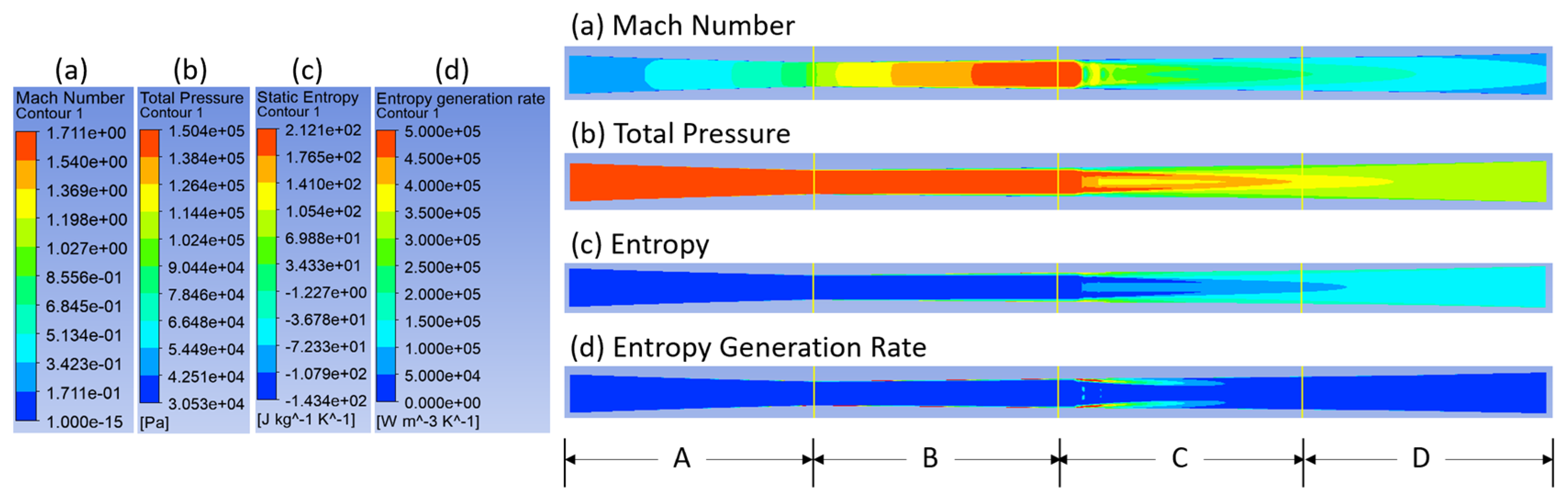
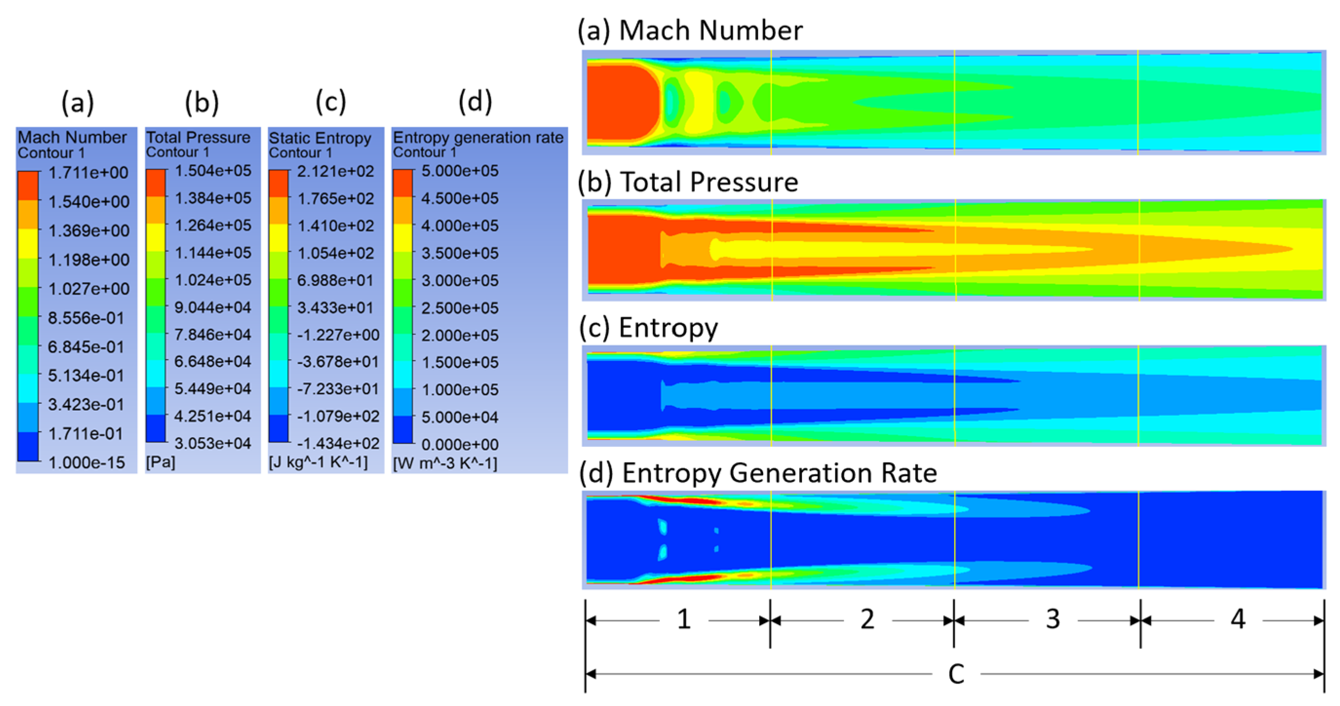
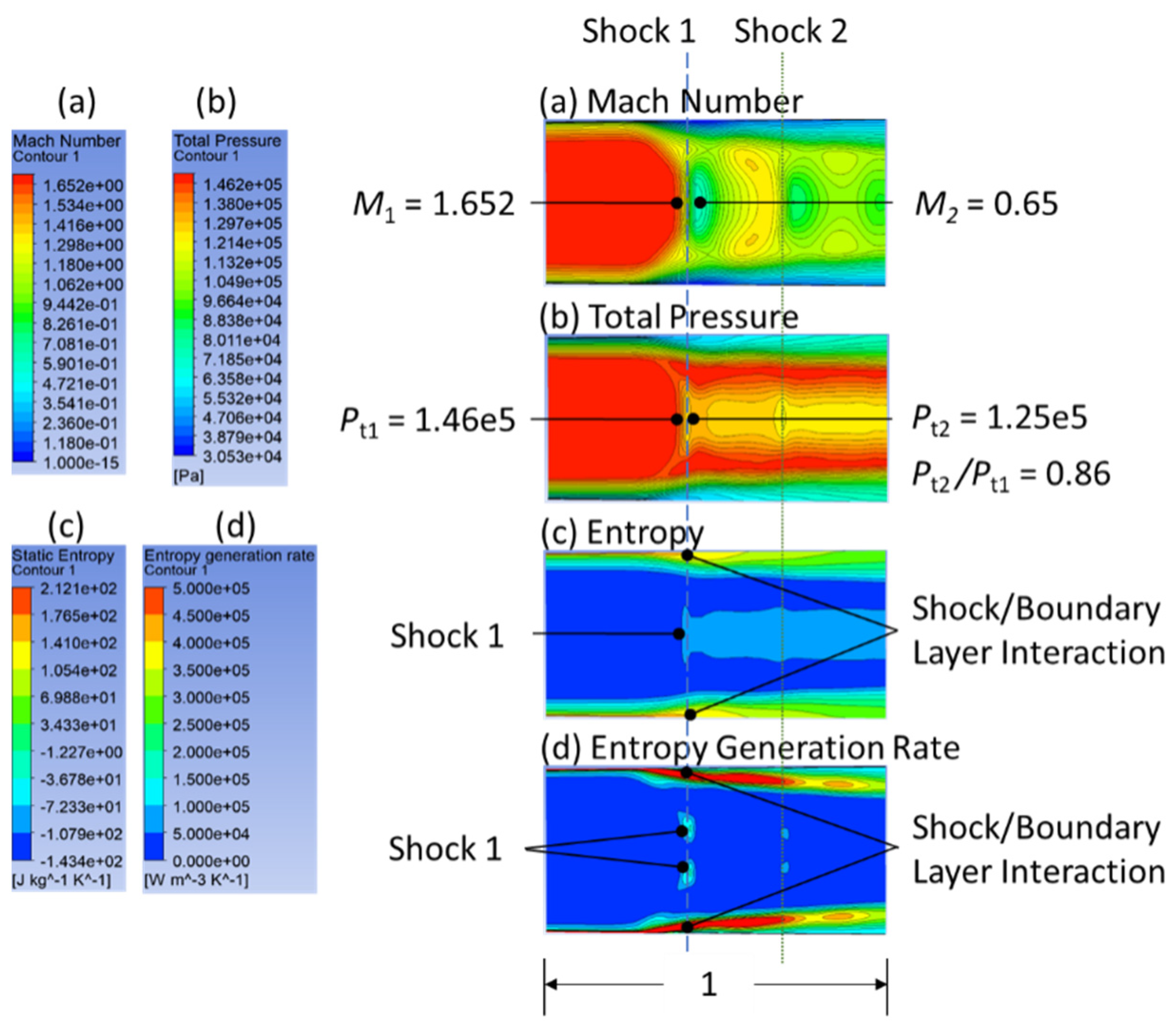
2.2. Case Two: Turbulent Compressible Flows in a Convergent-and-Divergent Nozzle (Laval Nozzle)

This section investigates compressible flows with shock waves. According to Greitzer and Tan [7], the entropy generation mechanism in 1D shocks was studied as early as 1957 by Liepmann and Roshko [35] and numerically investigated by Teeple in 1995 [7]. Although the entropy generation mechanisms inside a shock wave are very complicated because rapid pressure and temperature changes occur within a thin layer that is only about five times the mean free path of air molecules, Teeple argues that the continuity assumption of gas dynamics still applies and states that the governing equations can be numerically integrated directly and that the results are reliable. Teeple concludes that, with an incoming Mach number M₁ = 1.5, the viscous dissipation and the heat transfer are responsible for about 60% and 40% of the total entropy generation across the shock, respectively, and this all occurs within five times the mean free path of molecules.

Given the impracticality of applying a direct Navier–Stokes simulation like what Teeple did to real-life machines such as axial compressors, we investigate the applicability of the differential approach to shocks when using commonly available CFD tools and turbulence models. The applicability of the differential approach is judged based on two criteria: (1) whether the grid independence is based on the integrated entropy generation across the control volume under concern and (2) whether the Mach number and the total pressure ratio across the shock are consistent with the 1D theory. Two details are ignored: (i) The contributions of viscous dissipation and heat transfer are not separated, and (ii) the length scale of the shock wave is in the length of a few grids rather than a multiple of the mean free path of molecules. For practical purposes, the contributions of viscous dissipation and heat transfer within the shock waves do not need to be distinguished. Instead, identifying the sources of loss by distinguishing the contribution of a shock as a whole from the others is essential.

A Laval nozzle with an adiabatic wall boundary is the second test case. The y+ < 300. The flow residual is set as 1.0 × 10⁻⁵. The inlet and outlet diameters are 0.04 m, and the throat diameter is 0.02 m. The length of the convergent section before the throat is 0.3 m, and the length of the divergent section after the throat is 0.7 m. A 0.7-m-long straight pipe is placed in front of the Laval nozzle to accommodate the entrance effect, while a 0.7-m-long straight pipe is placed behind the Laval nozzle to prevent reflective waves from the exit. Thus, the entire pipe is naturally divided into three sections (I, II, and III), as shown in Figure 2. Section I is the entrance section, section II is the Laval nozzle, and section III is the exit section. To display the simulation results later, the Laval nozzle is further divided into four sections (Figure 2). If the throat position is defined as x = 0, section A is between $-0.2$ to 0 m, section B is between 0 and 0.2 m, section C is between 0.2 to 0.4 m, and section D is between 0.4 and 0.6 m.

In this test case, the fluid is air and the flow is supersonic. To ensure that a shock is present inside the nozzle, an exit static pressure at 0.1013 MPa and an inlet total pressure of 0.15 MPa are chosen to create a shock inside the nozzle. The inlet’s total temperature is 288.15 K. In the CFD algorithm, the k–ε turbulence model is chosen. Structural grids are generated, wherein two O-type grid divisions are used in the circular cross usection to ensure good mesh quality. Grid independence is verified with respect to the overall entropy generation inside the entire computational domain. Two million grids are verified to suffice with respect to other flow parameters, such as the total pressure ratio. However, the grid density does not suffice for independence with respect to the entropy generation until the total number of grids is 9.3 million. Figure 3 shows the process for verifying grid independence, where the ordinate is the overall entropy generation, which is the integral of the volumetric EGR over the entire computational domain. The grid density first increases in the cross section of the pipe and then gets increasingly dense in the axial direction. The figure also shows the EGR contours (per unit volume). The variations in these contours with increasing grid numbers are also shown. The label of the color maps is the same as that in Figure 4, Figure 5 and Figure 6. Subsequently, the total grid number of 9.3 million is chosen for further study. If independence is desired with respect to other flow parameters, such as mass flow rate, 2 million grids suffice, which is much less than for EGR.

According to 1D inviscid aerodynamics, two critical back pressures exist: P_c and P_h. When the actual back pressure P_b is greater than or equal to P_c, the flow in the nozzle is subsonic; when P_b ≤ P_h, the flow is supersonic, and when P_c < P_b < P_h, a standing shock occurs in the divergent section. In our test case, P_c = 0.148 MPa and P_h = 0.004355 MPa, which is predicted by the 1D inviscid theory. Thus, shocks occur when the actual back pressure is between P_c and P_h. The numerical results indicate that this is the case for the given boundary conditions (Figure 4). The shock appears clearly in the Mach number and total pressure contours. However, the numerical results reveal two shock waves, the second of which stems from the shock-boundary-layer interactions. Such interactions induce boundary-layer separation behind the shock, which blocks part of the flow channel such that the local flow experiences a new convergent-divergent section. The second shock is the consequence of the new convergent-divergent section.

Figure 4c,d show the contours of entropy and EGR calculated with the differential approach. We analyze in particular the behavior of the EGRs around the shocks. Section C, where the shocks are located, is magnified, and the contours for this section are shown in Figure 5. The results show that both the largest entropy and the largest EGR occur around the shocks along the solid boundary, and they gradually grow toward the pipe center. The shocks themselves do not produce the sharpest variations in entropy, which means that the EGRs of the shocks are not the largest in this flow field.

Surprisingly, a strong normal shock itself does not produce the largest EGR, which seems counterintuitive. This is verified by checking the normal shock against the 1D theory. Although the flows in the Laval nozzle in this simulation are three-dimensional, the shock at the axisymmetric center line should closely follow the relation of a 1D normal shock. Thus, the CFD results are initially verified by matching the Mach number and total pressure ratio with the 1D theory. To demonstrate unambiguously the flow structures around the shocks, section C is further divided into four subsections, where the shocks all occur within subsection 1. According to the 1D theory, when the Mach number M₁ = 1.65 before a normal shock, the Mach number immediately after the shock should be M₂ = 0.65, and the total pressure ratio should be 0.86, as observed in Figure 6, which shows a magnified view of subsection 1 of Figure 5. This means that our numerical results correctly capture the shock. Thus, the solutions for the pressure and Mach number and other flow properties are reliable.

Entropy contours help understand the loss sources in the Laval nozzle. Since entropy is a state property of the fluid, it depends only on the local fluid properties such as pressure and temperature. As stated above, the solutions for pressure, temperature, and other parameters of our numerical simulations are correct. Therefore, the entropy results are reliable. Figure 5c and Figure 6c show that the local entropy most rapidly increases on and near the solid boundary, followed by the location of Shock 1. According to thermodynamics, in an adiabatic flow, the entropy gradient over a spatial distance is the EGR, which is exactly the case shown in Figure 5d and Figure 6d. Thus, the results of the differential approach for the EGRs are accurate, provided that the grids are sufficiently dense to capture the shocks and the shock–boundary-layer interaction.

3. Identification of Loss Sources in an Axial Compressor Rotor

The flow fields of R67, a typical transonic rotor, contain rich flow structures, such as leading tip flow, leakage flow, wake flow, limiting streamline, corner vortex, shock waves, and shock–boundary-layer interactions. Therefore, R67 is an ideal test case for demonstrating how the loss sources can be identified with the differential approach when considering flow fields as complicated as those of R67. The losses inside axial compressors have always been an important research topic. Nevertheless, due to the lack of direct measurements, compressor losses can only be calculated as a whole, such as compressor efficiency, or displayed with the color contours of entropy. The differential approach thus provides a new alternative for determining the loss sources within axial compressors. In this section, the flows of R67 near peak efficiency are chosen and interesting flow features are discovered, some of which cannot be visualized without using the differential approach.

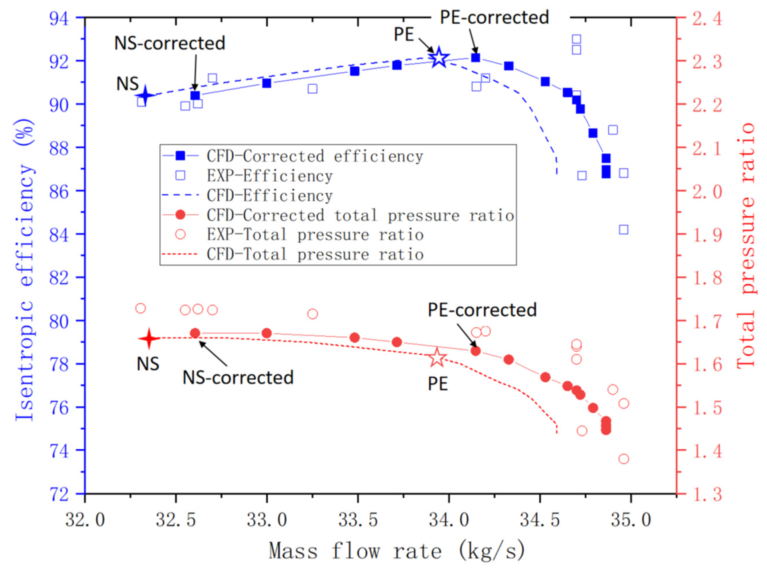
3.1. Validation of Numerical Simulation

The model of R67 is shown in Figure 7. R67 is designed to rotate at 16,043 rpm, and the number of blades is 22. R67 is simulated and validated with experimental data. The boundary is set up as follows: The total inlet pressure is fixed at 0.1013 MPa and the total temperature is 288.15 K. The outlet pressure can be varied to obtain different compressor conditions. The shear stress transport turbulence model is chosen, and grid independence is first verified. Like the previous sections, grid independence is based on the overall entropy generation. Entropy generation vs. mesh number is plotted in the upper-right corner of Figure 8, and the data are listed in

Table 1. Compressor characteristics for different mesh numbers.

Mesh Number (Million)	Mass Flow (kg/s)	Efficiency (%)	Total Pressure Ratio	Entropy Generation of Rotor Passage (W/K)	Percentage of Entropy Generation Variance (%)
4.76	34.31	90.6	1.54	17.5	−5.3
8.98	34.39	90.6	1.54	18.16	−1.73
11.11	34.38	90.6	1.54	18.48	base
15.76	34.38	90.6	1.54	18.55	0.38

. The back pressure is set at 0.1100 MPa. Grid independence in terms of the regular criteria, such as total pressure ratio and/or efficiency, is attained at a mesh number of 4.76 million. However, if entropy generation is the criterion, grid independence is attained at 11.11 million meshes. Figure 8 displays the EGR distributions along the axial chord for four different mesh numbers. As the grid is refined, the curves first converge upstream of the tip’s trailing edge, whereas the curves are most difficult to converge downstream of the trailing edge.

Figure 9 plots the rotor characteristics. The experimental data were taken from NASA’s original 1991 report [36], and the rotor speed is corrected from 16,043 to 16,169 rpm. The CFD results are also corrected for comparison with the experimental results. The correction is carried out based on the following compressor similarity rules:

$$Q=\frac{n}{n_0}{Q}_0,$$

(21)

$$\pi ={\left[1+{\left(\frac{n}{n_0}\right)}^2\left({\pi }_0{}^{\frac{n-1}{n}}-1\right)\right]}^{\frac{n}{n-1}},$$

(22)

where Q and π refer to the mass flow and total pressure ratio, respectively, and the rotation speed is 16,169 rpm. The subscript 0 identifies the parameter of the 16,043 rpm rotation speed.

Although the validation with the experimental data was performed with the corrected rotor speed, the flow analysis in the next section is carried out at the design speed at which the CFD is conducted. In Figure 9, the points PE (peak efficiency), PE-corrected, NS (near stall), and NS-corrected are both marked on their respective curves. The overall simulated total pressure ratio and efficiency are close to the experimental data. In this paper, we choose PE as the case to analyze the flow field in the next section.

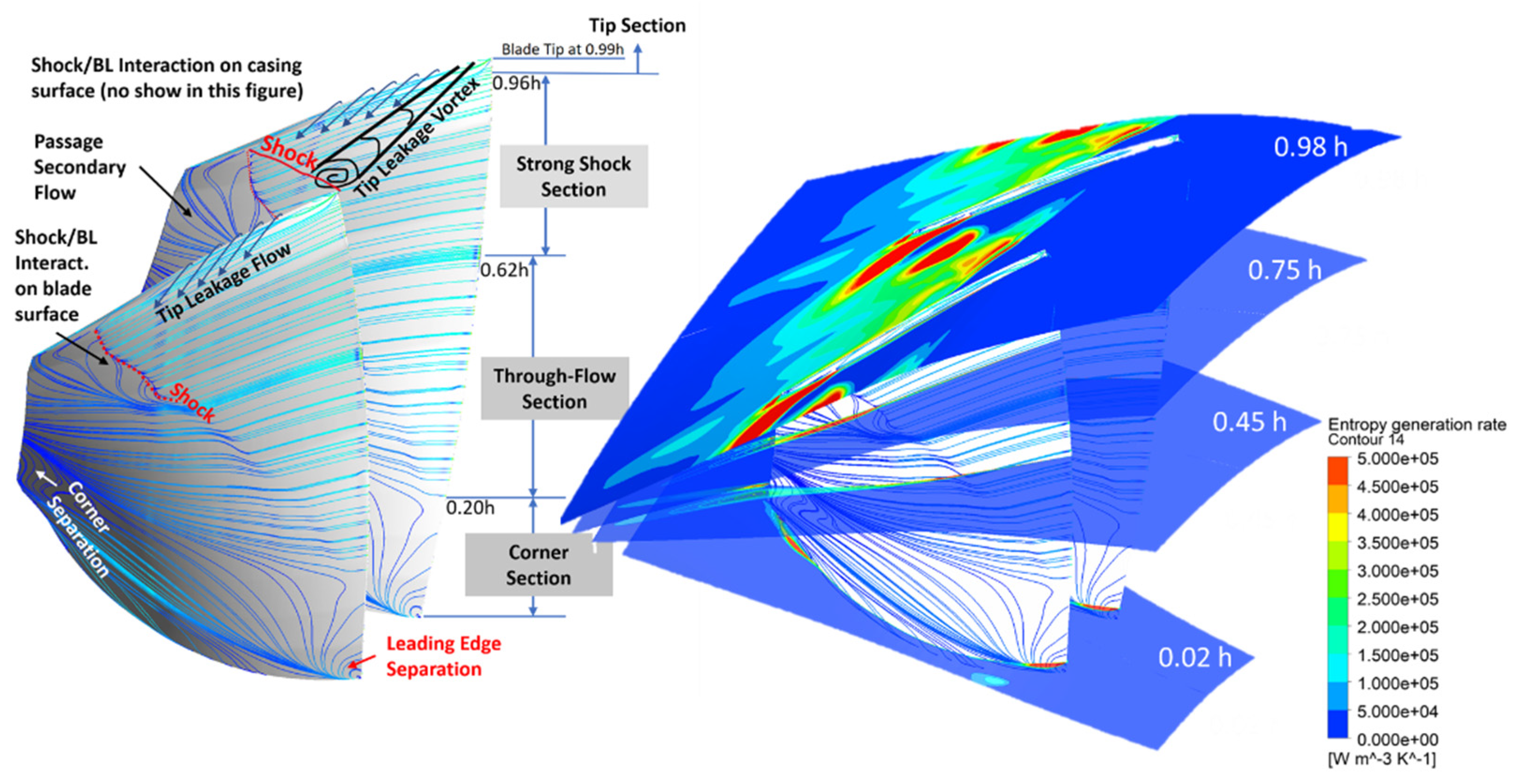
3.2. Flow Structures and Loss Sources

Figure 10 divides the flow field into four sections from the tip to the hub along the leading edge of the blade span: (1) tip section (0.96h–1.00h); (2) strong shock section (0.62h–0.96h); (3) through-flow section (0.20h–0.62h); and (4) corner section (0.00h–0.20h). Here, h is the span at the leading edge with the hub at 0.00h and the casing at 1.00h. Such divisions are not strict but derive only from the observation of the limiting streamline patterns on the suction surface of the blade. Thus, the divisions are only for the convenience of the qualitative description of the flow structures. The patterns of the limiting streamlines are commonly used as a measure to observe the flow structures. The left-hand side of Figure 10 shows that the following flow structures are present in each section:

(1)

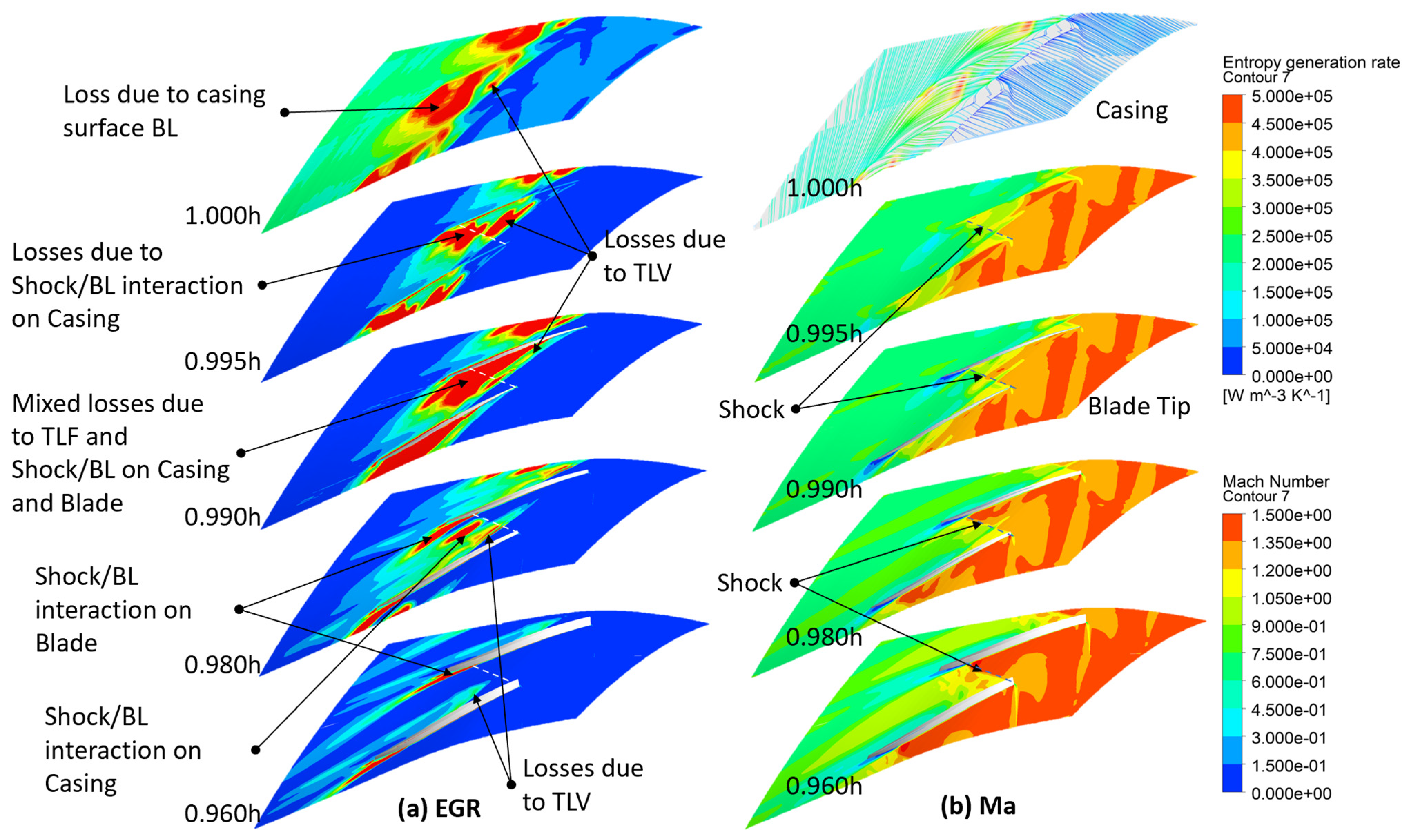
Tip section: Tip leakage flow, wherein a tip leakage vortex is initiated near the leading edge [19,20,21,22,23]; shock, and shock–boundary-layer interaction on the casing surface and on the blade’s suction surface. Some of the aforementioned flow structures cannot be directly observed from the limiting streamlines on the blade surface. However, they have been demonstrated in many studies because R67 has been widely studied worldwide ever since its data were made accessible to the public over 30 years ago.

(2)

Strong shock section: shock and shock–boundary-layer interaction on the suction surface; passage secondary flow near the trailing edge [29,30,31].

(3)

Through-flow section: most simple and clean flow with only a weak shock.

(4)

Corner section: leading-edge separation; corner separation near the trailing edge [26,28].

Figure 10. Flow structures in R67 at PE and the typical contours of EGRs.

Figure 10. Flow structures in R67 at PE and the typical contours of EGRs.

In addition to the above flow structures, wakes are always present along the trailing edge and are thus not listed repeatedly in each section. Figure 10 shows the four streamwise surfaces (S1 surfaces) on the right side, one for each section, on which the EGR contours are plotted. The contours are a convenient method to display the flow structures and their contributions to the losses.

Table 2. Comparison of entropy generation for the sections.

Section	Entropy Generation (W/K)	Percentage
Tip (0.631.00h)	4.71	27%
Strong Shock (0.62–0.96h)	6.26	36%
Through-Flow (0.20–0.62h)	4.3	24%
Corner (0.00–0.20h)	2.34	13%
TOTAL	17.61	100%

lists the entropy generation for each section. The largest entropy generation stems from the strong shock section, whereas the second largest stems from the tip section, followed by the through-flow section and the corner section. Since the tip section occupies the least volume, the EGR in this section is the most intensive, followed by the strong shock section. The flow structures within the through-flow section and the corner section are important because these two sections together generate 37% of the entropy. However, due to page limitations, they are not analyzed in detail herein.

3.2.1. Details in the Tip Section

Among the four contours in Figure 10, the flow structures on 0.98h are the most noticeable, indicating that the flows in the tip section are the most complicated and the EGRs are the most intensive. Thus, Figure 11 shows the details of the tip section. Five surfaces are plotted: 1.000h = the casing surface (also called the shroud surface); 0.995h = the mid-span of the tip gap; 0.990h = the blade tip; 0.980h = a surface within the tip section, and 0.960h = the bottom surface of the tip section. All contours are plotted on three-dimensional curvy surfaces with the same viewing angle as Figure 10. The left column displays the EGR (Figure 11a) while the right column displays the Mach number (Figure 11b). However, one exception exists: since there is no absolute velocity on the casing, the contour of the Mach number on the casing is replaced by the limiting streamlines.

Figure 11 is quite busy because the flow structures within this narrow region are complicated. The surface of the blade tip (0.990h) divides the tip section into two parts. The upper part comprises the flow within the tip gap, whereas the lower part comprises the flows influenced by the tip leakage flow and tip leakage vortex. The EGR contours on the casing surface are mostly due to the skin friction on the turbulence boundary layer, which is usually very strong. On the surface within the tip gap (0.995h), a shock appears from the Mach number contour. A black dotted line marks the shock, which is copied and shifted parallel to the left, marking the same shock location on the EGR contour. Inside the tip gap, the influence of the casing boundary layer is very strong and the loss due to the tip leakage vortex is distinguishable.

As illustrated in Figure 10, the flow structures in the tip section include the tip leakage flow, tip leakage vortex, shock, and shock–boundary-layer interactions with the casing and the blade’s suction surface. On the tip surface (0.990h), all these losses are mixed and barely distinguishable. However, on the surface at 0.980h, they are separated because the flows are within the blade passage. Here, the influence of the casing boundary layer weakens and the blade boundary layer starts to dominate. The tip leakage flow and tip leakage vortex also gradually weaken. Farther along the surface of 0.960h, the casing influence cannot be traced, and the tip leakage vortex is almost wiped out, whereas the shock–boundary-layer interaction on the blade surface becomes dominant.

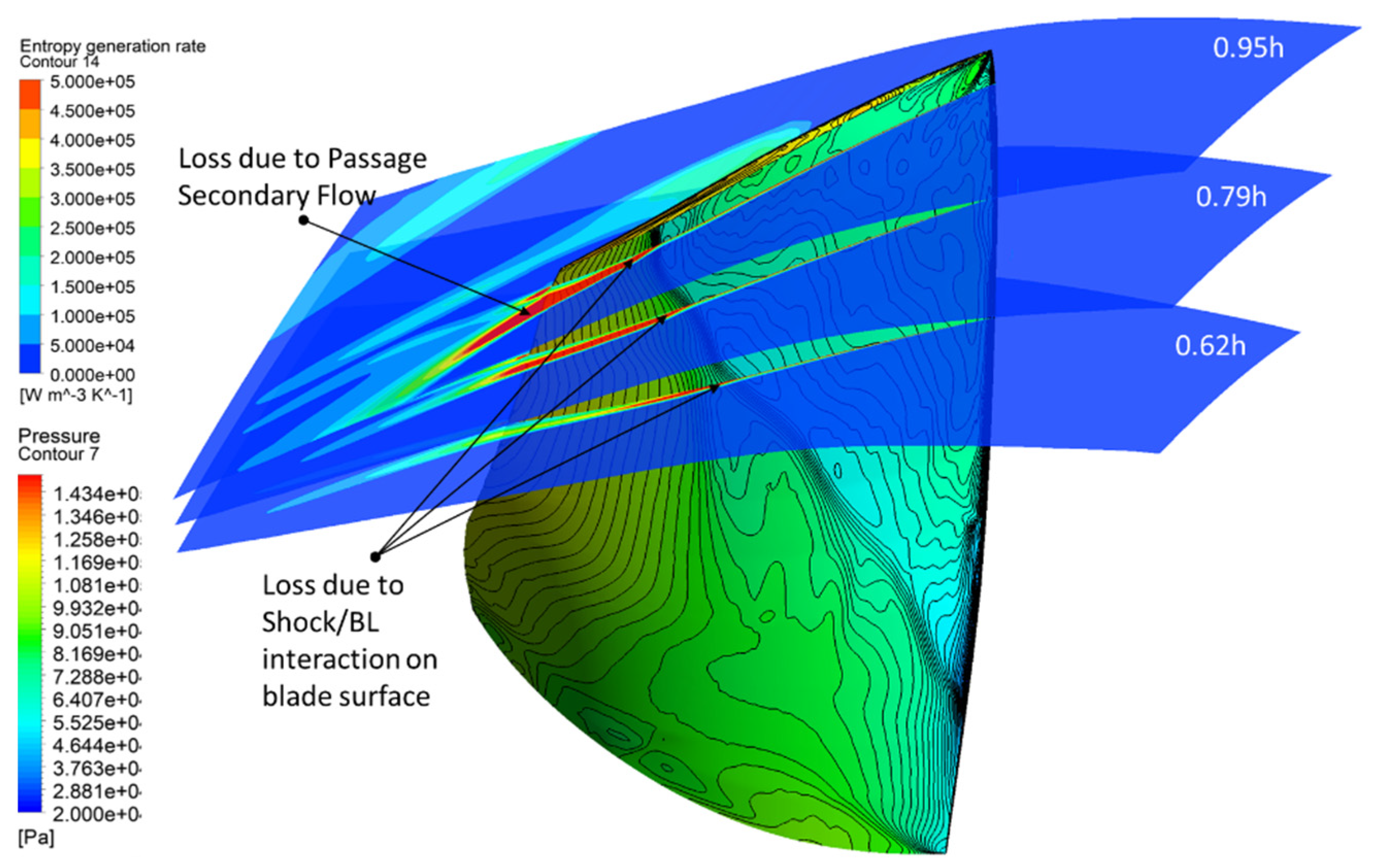
3.2.2. Details in the Strong-Shock Section

Figure 12 depicts the shock–boundary-layer interaction in the strong-shock section. The blade’s suction surface is covered with contours of static pressure through which the location of the shock across the blade span appears clearly. Figure 12 plots with EGR contours three streamwise surfaces within this section. The shock triggers boundary layer separation right after the shock wave, which leads to strong turbulent mixing downstream. The strength of the shock along the blade span is not uniform. The farther away from the tip, the weaker the shock. The EGR contours demonstrate this trend.

In the region behind the shock, the limiting streamlines on the blade’s suction surface show that a secondary flow exists and it causes the streamlines to move upward (Figure 13). In Figure 13, the radial planes (S3 surfaces) are added, and the EGR contours are plotted on these planes. This secondary flow is believed to be caused by the passage vortex.

This secondary flow contributes significantly to the overall loss.

To visually compare these radial EGR contours with the streamwise EGR contours due to the shock–boundary-layer interaction, Figure 14 plots a magnified view of these two EGR surfaces. Figure 14 shows how the two loss mechanisms merge near the blade surface. The combined turbulent flow turns toward the center of the passage due to the passage vortex, making the strong EGR contours turn 90° and overlap with the casing boundary layer.

4. Summary and Conclusions

This study carefully analyzes the differential approach of entropy generation. After considering two test cases, the differential approach is applied to R67, a transonic rotor. In the first test case, the differential approach was applied to laminar and turbulent flows in straight ducts. In the second test case, a convergent-divergent nozzle was studied. Finally, the differential approach was applied to a transonic rotor with shock waves. The results of the study lead to the following main conclusions:

(1)

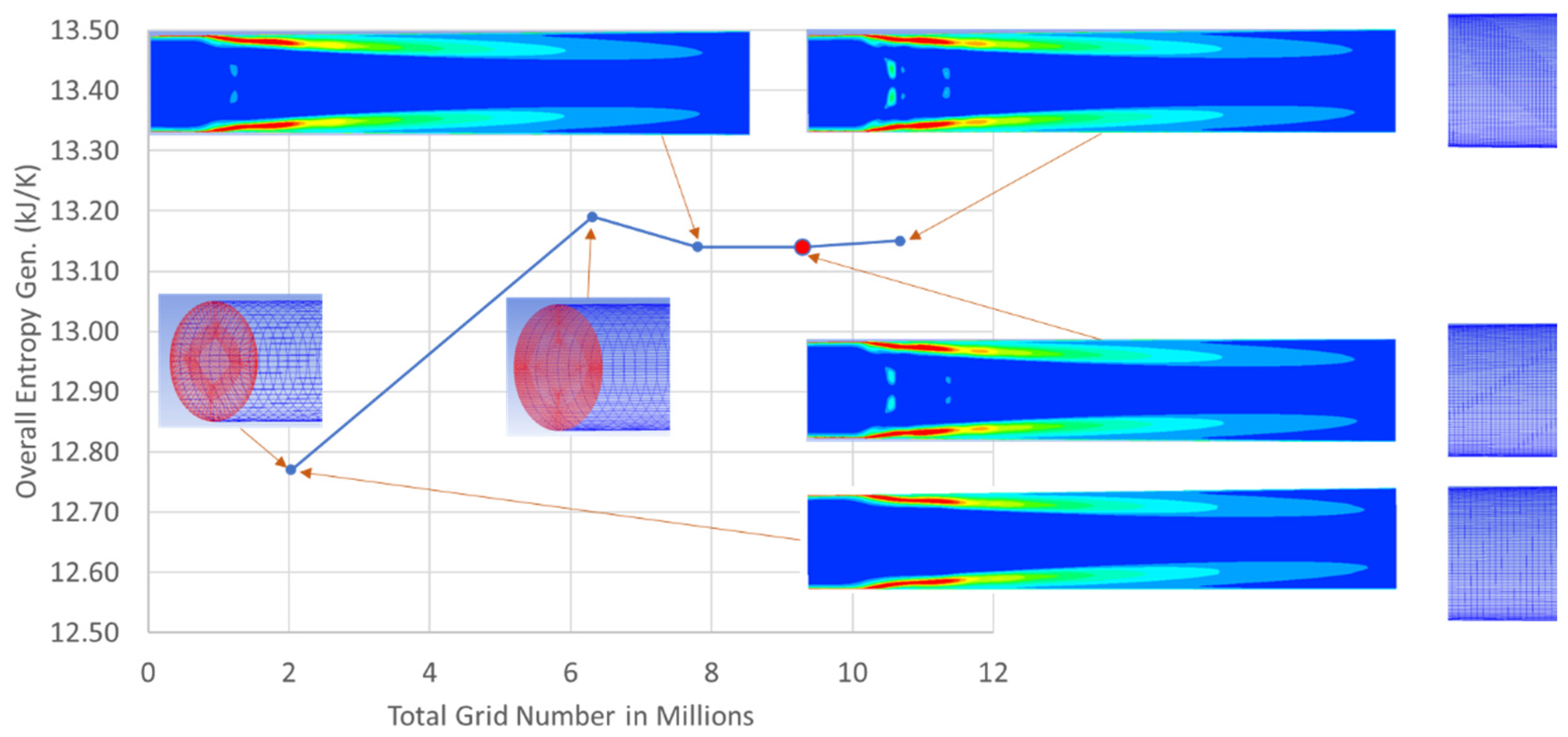
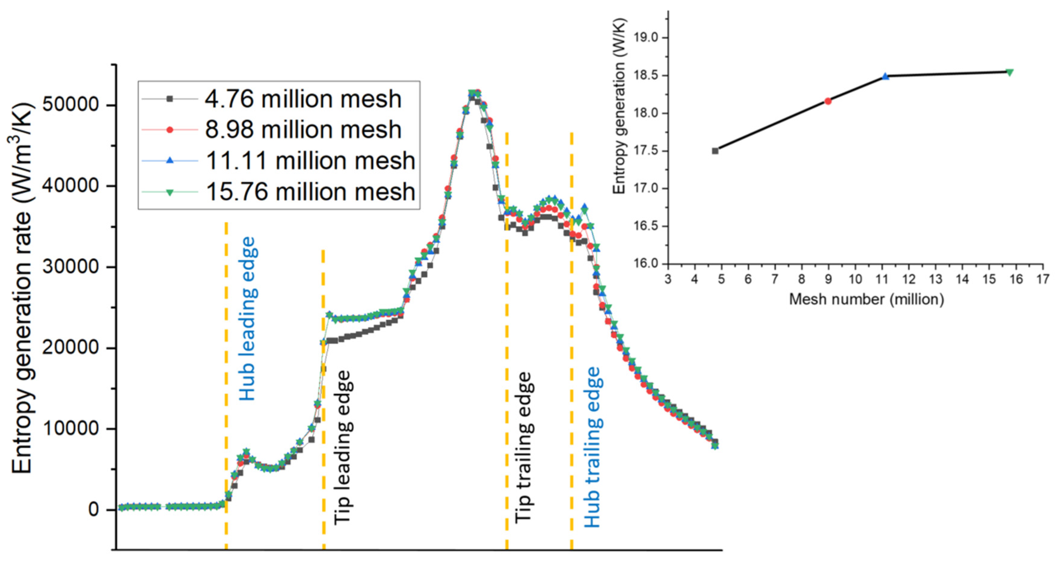
Grid Independence. Grid independence should not only be based on the common indicators but additionally on the overall entropy generation. The required number of grids (and the quality of the grids) is far greater than the normal number.

(2)

Test Case 1—Straight Ducts. The results of straight ducts show that the differential approach results are qualitatively consistent with the experimental data (the Moody chart) for both laminar and turbulent flows (only with a smooth wall). Therefore, the differential approach should be used as a tool for qualitative comparison rather than for quantitative design.

(3)

Test Case 2—Laval nozzle. The EGR due to the shock itself is much lower than that of the separation induced by the shock–boundary-layer interaction. In other words, the turbulence caused by the separation produces far more loss than the irreversibility across the shock waves. This is a key feature for identifying the loss sources within the transonic rotor R67.

(4)

R67 at near Peak Efficiency.

a.

About 63% of the total loss stems from the upper 0.38h of the blade span (0.62h–1.00h), which is mainly due to the shock–boundary-layer interaction on the casing and on the blade’s suction surface, tip leakage flow, tip leakage vortex, and passage secondary flow. The remaining 37% loss is produced by the main blade span (0.2h–0.62h). The corner section (0h–0.2h), which includes the corner separation, accounts for only 13% of the loss, which is surprising because this is quite different from the results of the cascade research. Therefore, the above loss-source identification indicates that the casing boundary layer makes an important contribution to the overall entropy generation. Loss-source identification indicates that the casing boundary layer makes an important contribution to the overall entropy generation. It interacts with the shock, the tip leakage flow, and the tip leakage vortex, all of which are major sources of loss.

b.

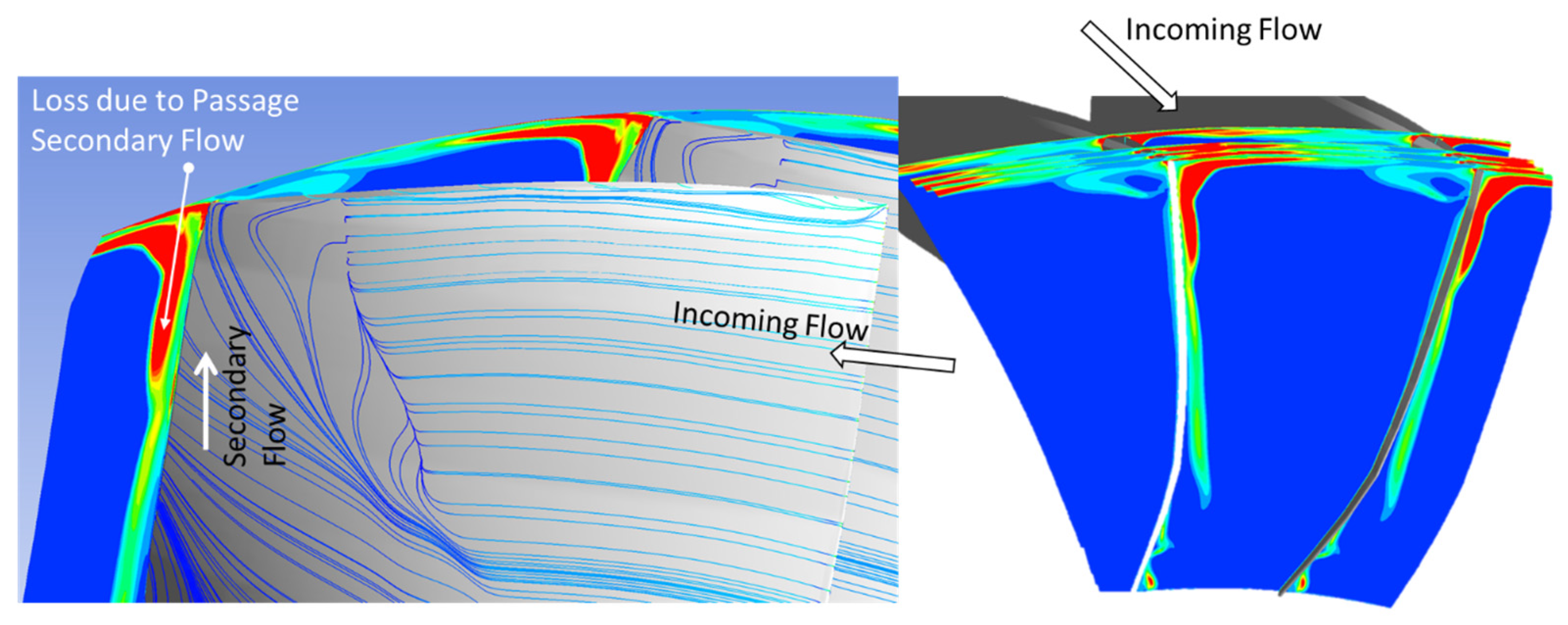
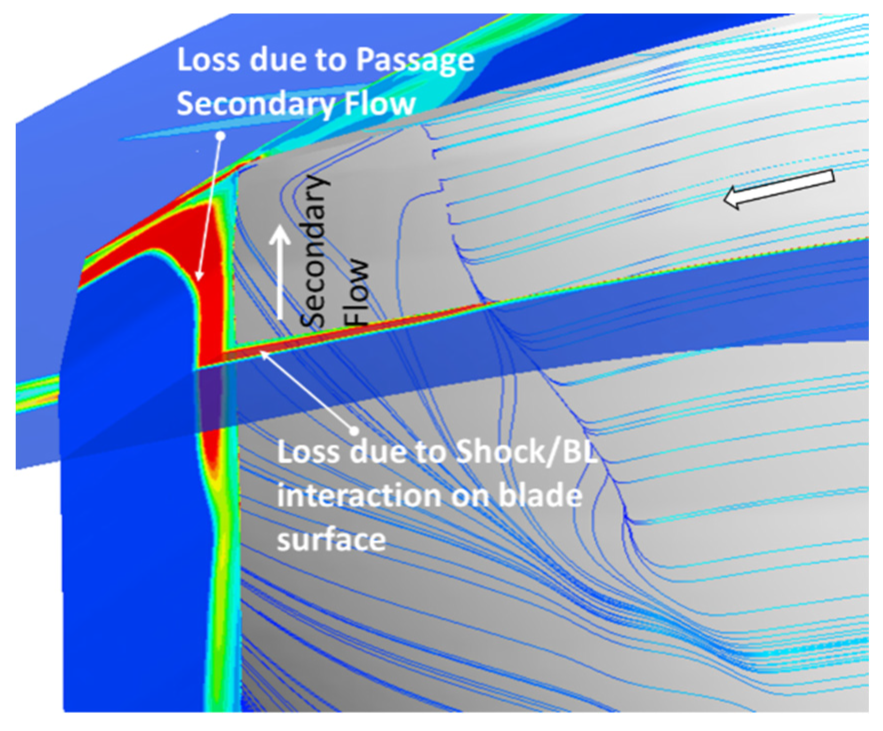
Passage secondary flow is a very important contributor to the total loss. Its loss is generated in the portion of the blade close to the trailing edge, which smoothly merges with the shock/boundary layer on the blade suction surface. Therefore, these two loss sources are barely separable. However, with the help of the differential approach, both these loss sources are determined to be equally important. This recalls a debate in 1991, where Li and Cumpsty [37] presented their measurements and argued that the circumferential mixing due to passage secondary vortex contributes the most loss in a large low-speed compressor stage. In contrast, Leylek and Wisler [38] demonstrated that both secondary flows and turbulent diffusion play important roles in the mixing process and contribute to both spanwise and cross-passage mixing. The relative importance of each of these two mechanisms depends on configuration and loading. Using the current CFD tool, the details of flow can be visualized and EGR contours can be plotted, providing a means to resolve the debate, as shown in this study.

References

1. Bejan, A. Entropy generation minimization: The new thermodynamics of finite size devices and finite time processes. J. Appl. Phys. 1996, 79, 1191–1218. [Google Scholar] [CrossRef] [Green Version]
2. Kock, F.; Herwig, H. Local entropy production in turbulent shear flows: A high-Reynolds number model with wall functions. Int. J. Heat Mass Transf. 2004, 47, 2205–2215. [Google Scholar] [CrossRef]
3. Herwig, H.; Schmandt, B. How to determine losses in a flow field: A paradigm shift towards the second law analysis. Entropy 2014, 16, 2959–2989. [Google Scholar] [CrossRef] [Green Version]
4. Schmandt, B.; Herwig, H. Losses due to conduit components: An optimization strategy and its application. J. Fluid Mech. 2016, 138, 031204. [Google Scholar] [CrossRef]
5. Jin, Y.; Du, J.; Li, Z.Y.; Zhang, H.W. Second-law analysis of irreversible losses in gas turbines. Entropy 2017, 19, 470. [Google Scholar] [CrossRef]
6. Geng, L.P.; Jin, Y.; Herwig, H. Can pulsation unsteadiness increase the convective heat transfer in a pipe flow? A systematic study. Numer. Heat Transf. Part B Fundam. 2020, 78, 160–174. [Google Scholar] [CrossRef]
7. Greitzer, E.M.; Tan, C.S.; Graf, M.B. Internal Flow; Cambridge University Press: New York, NY, USA, 2004. [Google Scholar]
8. Denton, J.; Pullan, G. A numerical investigation into the sources of endwall loss in axial flow turbines. In Proceedings of the ASME Turbo Expo 2012, Copenhagen, Denmark, 11–15 June 2012. [Google Scholar] [CrossRef]
9. Zlatinov, M.B.; Tan, C.S.; Montgomery, M.; Islam, T.; Harris, M. Turbine hub and shroud sealing flow loss mechanisms. J. Turbomach. 2012, 134, 061027. [Google Scholar] [CrossRef]
10. Lin, D.; Yuan, X.; Su, X.R. Local entropy generation in compressible flow through a high pressure turbine with delayed detached eddy simulation. Entropy 2017, 19, 29. [Google Scholar] [CrossRef] [Green Version]
11. Zhang, L.; Lang, J.H.; Jiang, K.; Wang, S.L. Simulation of entropy generation under stall conditions in a centrifugal fan. Entropy 2014, 16, 3573–3589. [Google Scholar] [CrossRef] [Green Version]
12. Wang, H.; Lin, D.; Su, X.R.; Yuan, X. Entropy analysis of the interaction between the corner separation and wakes in a compressor cascade. Entropy 2017, 19, 324. [Google Scholar] [CrossRef] [Green Version]
13. Li, Z.Y.; Du, J.; Jemcov, A.; Ottavy, X.; Lin, F. A study of loss mechanism in a linear compressor cascade at the corner stall condition. In Proceedings of the ASME Turbo Expo 2017: Turbine Technical Conference and Exposition, Charlotte, NC, USA, 26–30 June 2017. [Google Scholar] [CrossRef]
14. Zhang, Q.F.; Du, J.; Li, Z.H.; Li, J.C.; Zhang, H.W. Entropy generation analysis in a mixed-flow compressor with casing treatment. J. Therm. Sci. 2019, 28, 915–928. [Google Scholar] [CrossRef]
15. Ma, W.; Ottavy, X.; Lu, L.P.; Leboeuf, F.; Gao, F. Experimental investigations of corner stall in a linear compressor cascade. In Proceedings of the ASME 2011 Turbo Expo: Turbine Technical Conference and Exposition, Vancouver, BC, Canada, 6–10 June 2011. [Google Scholar] [CrossRef]
16. You, D.; Wang, M.; Moin, P.; Mittal, R. Large-eddy simulation analysis of mechanisms for viscous losses in a turbomachinery tip-clearance flow. J. Fluid Mech. 2007, 586, 177–204. [Google Scholar] [CrossRef] [Green Version]
17. Katiyar, S.; Sarkar, S. Flow transition on the suction surface of a controlled-diffusion compressor blade using a large-eddy simulation. Phys. Fluids 2022, 34, 094108. [Google Scholar] [CrossRef]
18. Zhu, H.L.; Zhou, L.; Meng, T.T.; Ji, L.C. Corner stall control in linear compressor cascade by blended blade and endwall technique based on large eddy simulation. Phys. Fluids 2021, 33, 115124. [Google Scholar] [CrossRef]
19. Du, H.; Yu, X.; Zhang, Z.; Liu, B. Relationship between the flow blockage of TLV and its evolutionary procedures inside the rotor passage of a subsonic axial compressor. J. Therm. Sci. 2013, 22, 522–531. [Google Scholar] [CrossRef]
20. Gao, Y.; Liu, Y.; Zhong, L.; Hou, J.; Lu, L. Study of the standard k-ε model for tip leakage flow in an axial compressor rotor. Int. J. Turbo Jet-Engines 2016, 33, 353–360. [Google Scholar] [CrossRef]
21. Smith, M.H.; Pullan, G.; Grimshaw, S.D.; Greitzer, E.M.; Spakovszky, Z.S. The role of tip leakage flow in spike-type rotating stall inception. J. Turbomach. 2019, 141, 061010. [Google Scholar] [CrossRef] [Green Version]
22. Zhang, B.T.; Liu, B.; Mao, X.C.; Wang, H.J.; Yang, Z.H.; Li, Z.Y. Interaction mechanism between the tip leakage flow and inlet boundary layer in a highly loaded compressor cascade based on scale-adaptive simulation. Phys. Fluids 2022, 34, 116112. [Google Scholar] [CrossRef]
23. Ventosa-Molina, J.; Lange, M.; Mailach, R.; Fröhlich, J. Study of relative endwall motion effects in a compressor cascade through direct numerical simulations. J. Turbomach. 2021, 143, 011005. [Google Scholar] [CrossRef]
24. Niu, H.; Chen, J.; Xiang, H.; Du, G. Investigation of incoming boundary layer effects on the flow field of transonic compressor rotor. J. Eng. Therm. Energy Power 2021, 36, 60–68. [Google Scholar]
25. Hou, J.X.; Liu, Y.W.; Zhong, L.Y.; Zhong, W.B.; Tang, Y.M. Effect of vorticity transport on flow structure in the tip region of axial compressors. Phys. Fluids 2022, 34, 055102. [Google Scholar] [CrossRef]
26. Liu, Y.; Yan, H.; Liu, Y.; Lu, L.; Li, Q. Numerical study of corner separation in a linear compressor cascade using various turbulence models. Chin. J. Aeronaut. 2016, 29, 639–652. [Google Scholar] [CrossRef] [Green Version]
27. Wang, Z.; Geng, S.; Zhang, H. Effects of inlet boundary layer on corner flow in a linear compressor cascade. J. Propul. Technol. 2017, 38, 54–60. [Google Scholar]
28. Meng, T.; Li, X.; Zhou, L.; Zhu, H.; Li, J.; Ji, L. Large eddy simulation and combined control of corner separation in a compressor cascade. Phys. Fluids 2022, 34, 075113. [Google Scholar] [CrossRef]
29. Hou, J.; Zhou, C. Loss mechanism of low-pressure turbine secondary flows due to different incoming boundary layers. J. Eng. Gas Turbines Power 2020, 142, 101004. [Google Scholar] [CrossRef]
30. Gmelin, C.; Thiele, F.; Liesner, K.; Meyer, R. Investigations of Secondary Flow Suction in a High Speed Compressor Cascade. In Proceedings of the ASME 2011 Turbo Expo: Turbine Technical Conference and Exposition, Vancouver, BC, Canada, 6–10 June 2011; pp. 405–415. [Google Scholar]
31. Liesner, K.; Meyer, R.; Lemke, M.; Gmelin, C.; Thiele, F. On the efficiency of secondary flow suction in a compressor cascade. In Proceedings of the ASME Turbo Expo 2010: Power for Land, Sea, and Air, Glasgow, UK, 14–18 June 2010; pp. 151–160. [Google Scholar]
32. Krug, A.; Busse, P.; Vogeler, K. Experimental investigation into the effects of the steady wake-tip clearance vortex interaction in a compressor cascade. J. Turbomach. 2015, 137, 061006. [Google Scholar] [CrossRef]
33. Babu, S.; Chatterjee, P.; Pradeep, A.M. Transient nature of secondary vortices in an axial compressor stage with a tandem rotor. Phys. Fluids 2022, 34, 065125. [Google Scholar] [CrossRef]
34. White, F.M. Fluid Mechanics, 6th ed.; McGraw-Hill College: New York, NY, USA, 2006. [Google Scholar]
35. Liepmann, H.W.; Roshko, A. Elements of Gas Dynamics; John Wiley & Sons: New York, NY, USA, 1957. [Google Scholar]
36. Strazisar, A.J.; Wood, J.R.; Hathaway, M.D.; Suder, K.L. Laser Anemometer Measurements in a Transonic Axial-Flow Fan Rotor; NASA Technical Paper; NASA: Washington, DC, USA, 1989; p. 2879. [Google Scholar]
37. Li, Y.S.; Cumpsty, N.A. Mixing in axial flow compressors: Part I-test facilities and measurements in a four-stage compressor. J. Turbomach. 1991, 113, 161–165. [Google Scholar] [CrossRef]
38. Leylek, J.H.; Wisler, D.C. Mixing in axial-flow compressors: Conclusions drawn from three-dimensional Navier-Stokes analyses and experiments. J. Turbomach. 1991, 113, 139–143. [Google Scholar] [CrossRef]
Figure 1. Moody chart comparing the results of differential approach with data from [3] and with experimental results.
Machines 11 00472 g001
Figure 2. Coordinate system for Laval nozzle.
Machines 11 00472 g002
Figure 3. Grid independence with respect to overall entropy generation.
Machines 11 00472 g003
Figure 4. Distribution of Mach number, total pressure, entropy, and EGR within sections of the Laval nozzle.
Machines 11 00472 g004
Figure 5. Contours of Mach number, static pressure, static entropy, and EGR within section C of Figure 4.
Machines 11 00472 g005
Figure 6. Contours of Mach number, static pressure, static entropy, and EGR within subsection 1 of Figure 5.
Machines 11 00472 g006
Figure 7. R67 model.
Machines 11 00472 g007
Figure 8. Curve showing grid independence in terms of overall EGR and the selected grid.
Machines 11 00472 g008
Figure 9. Compressor characteristics validated with experimental data.
Machines 11 00472 g009
Figure 11. Contours of (a) entropy generation rate (EGR) and (b) Mach number (Ma). Some of the abbreviations are TLF = tip leakage flow, TLV = tip leakage vortex, and BL = boundary layer.
Machines 11 00472 g011
Figure 12. EGR contours in the strong-shock section.
Machines 11 00472 g012
Figure 13. Loss due to the passage secondary flow.
Machines 11 00472 g013
Figure 14. Magnified view of EGR contours on the two intersecting surfaces.
Machines 11 00472 g014