
Experimental and Numerical Analysis of Triply Coupled Vibration of Thin-Walled Beam with Arbitrary Closed Cross-Section
Abstract
:1. Introduction
2. Basics of the Theoretical and Mathematical Model
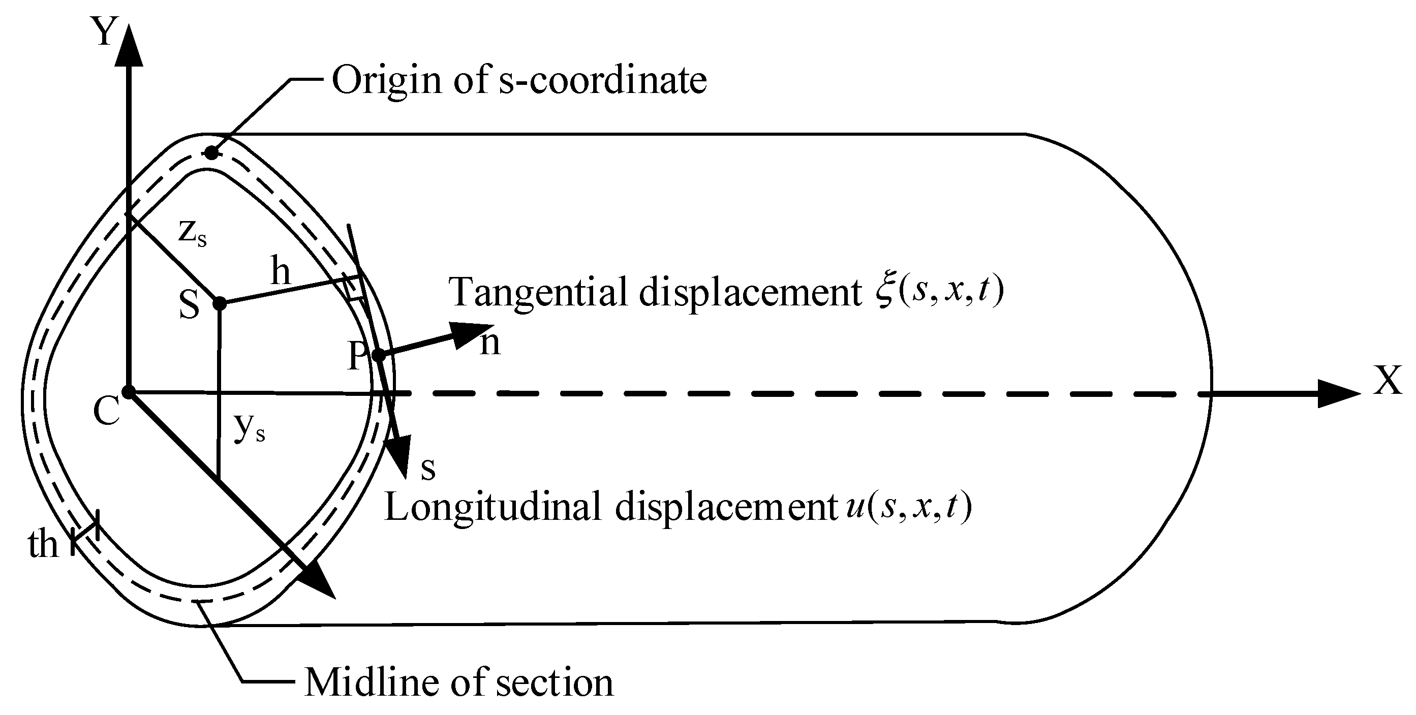
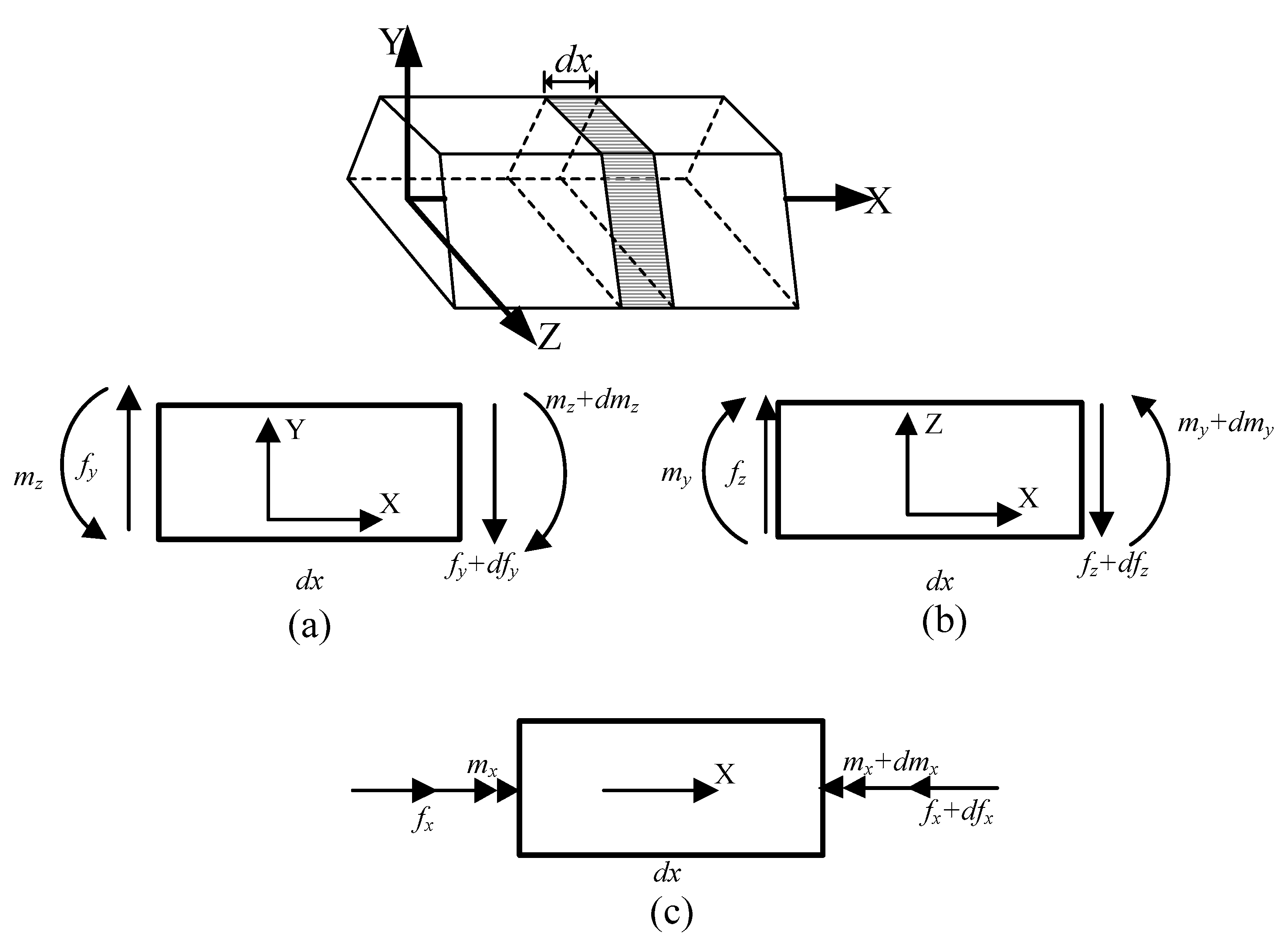
2.1. Equations of Motion
2.2. Free Vibration
2.3. Axial Vibration
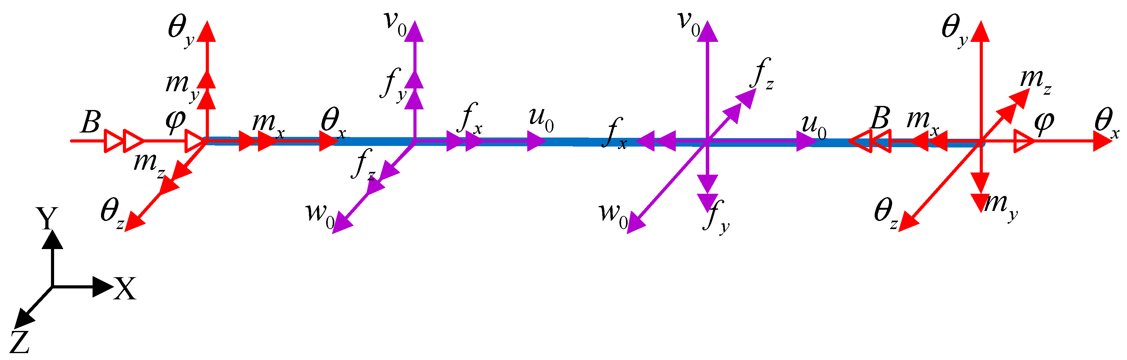
2.4. Dynamic Transfer Matrix Formulation
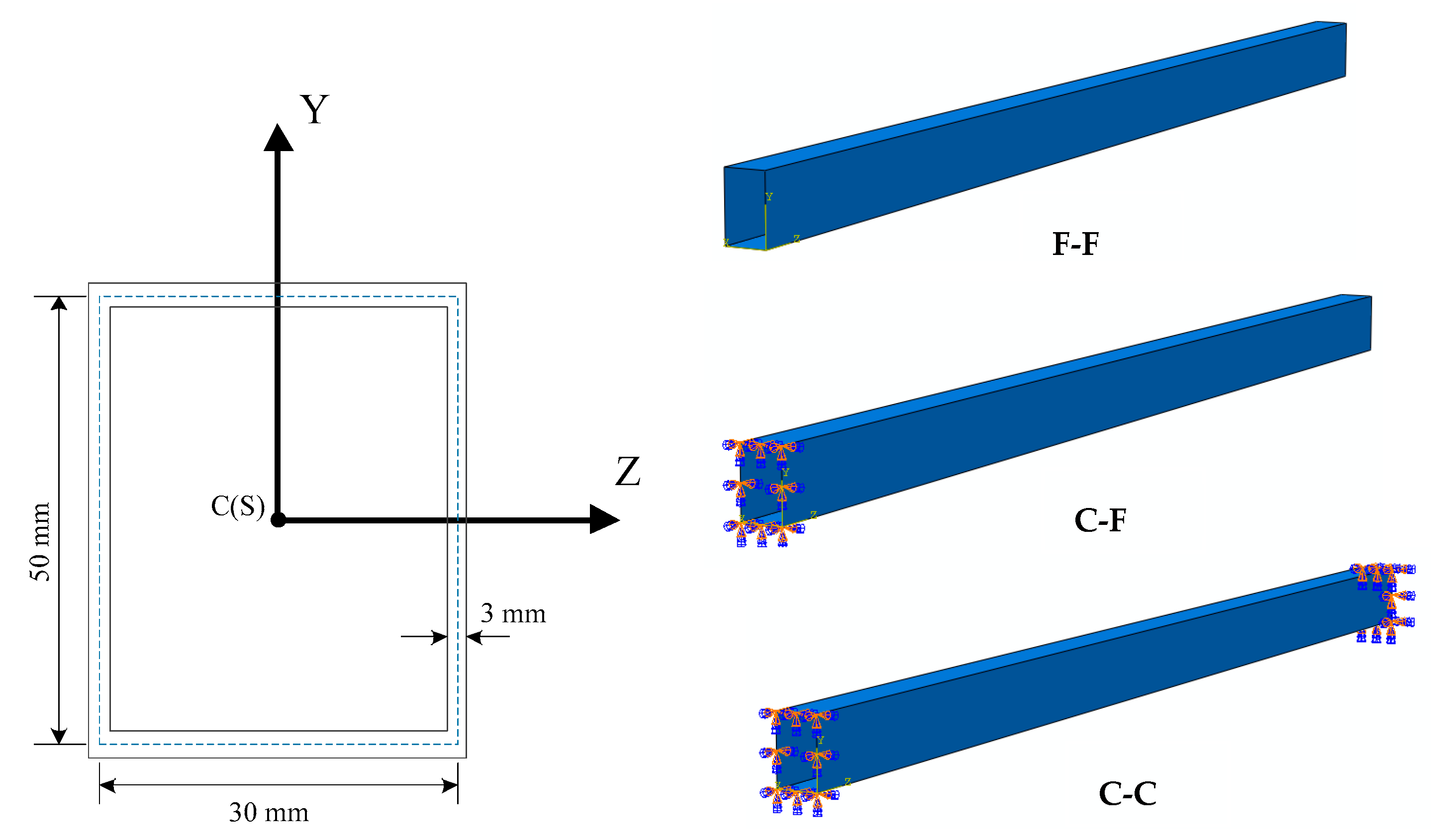
3. Boundary Conditions
4. Accuracy Verification and Numerical Examples
4.1. Example 1
4.2. Example 2
5. Experimental Model
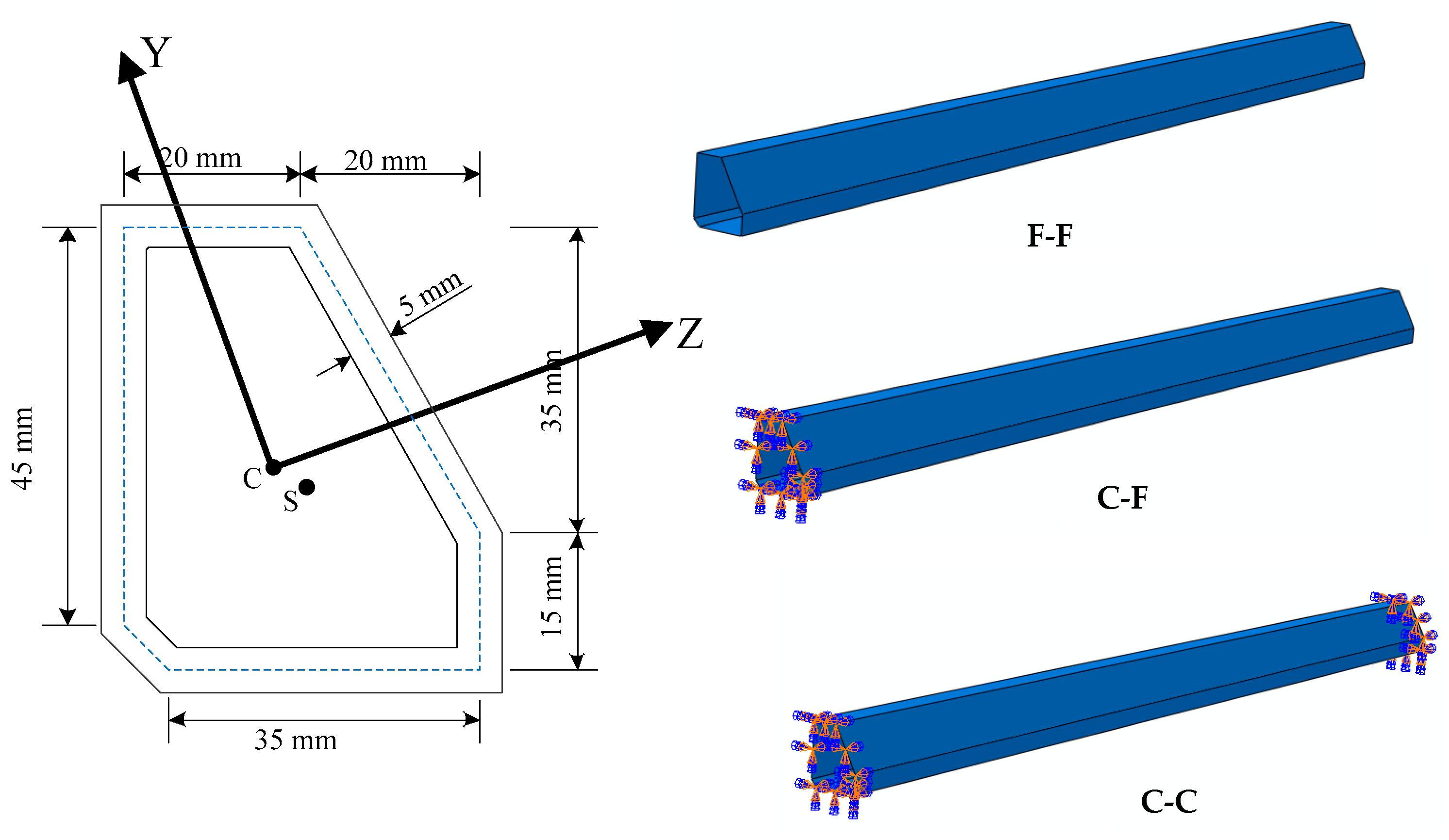
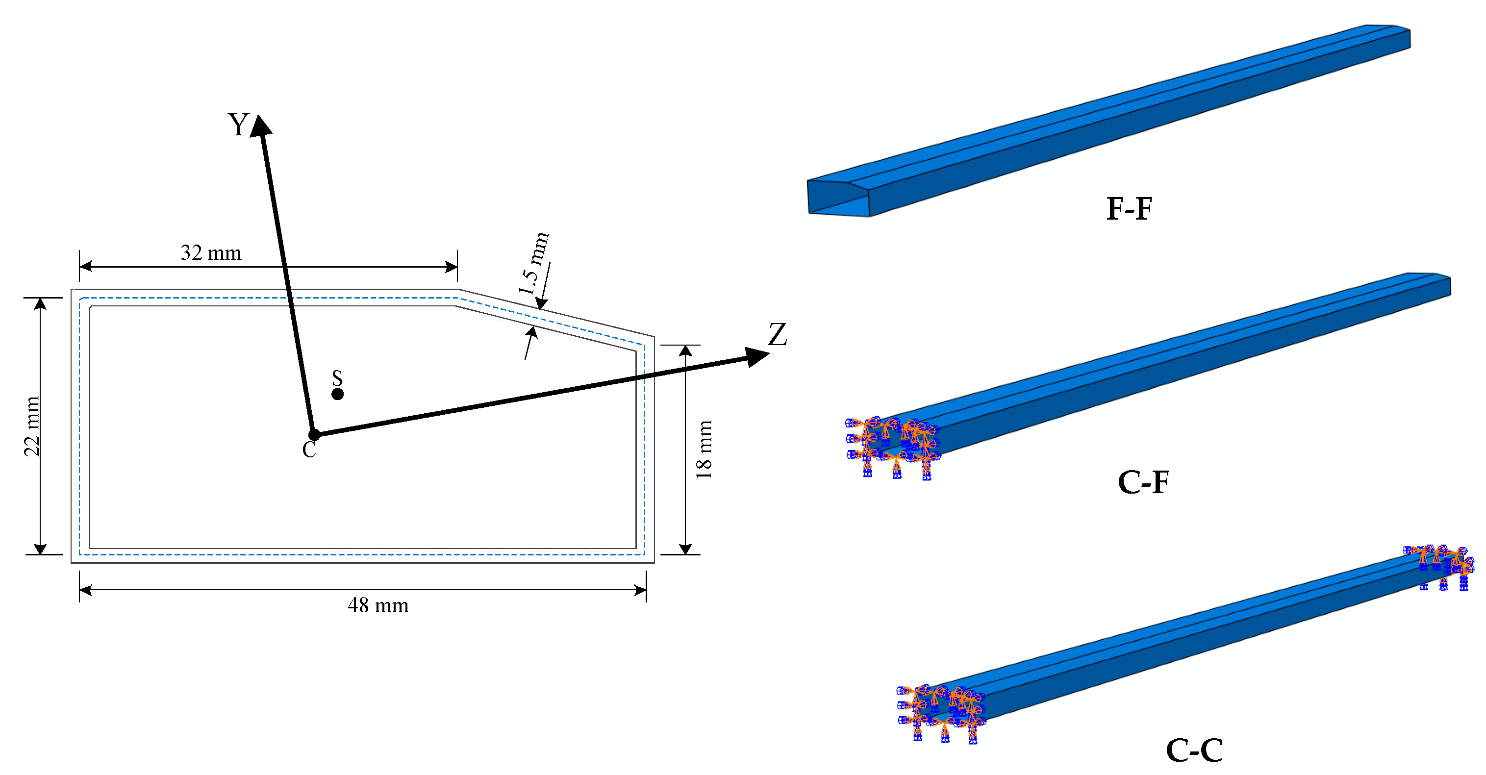
5.1. Case Study
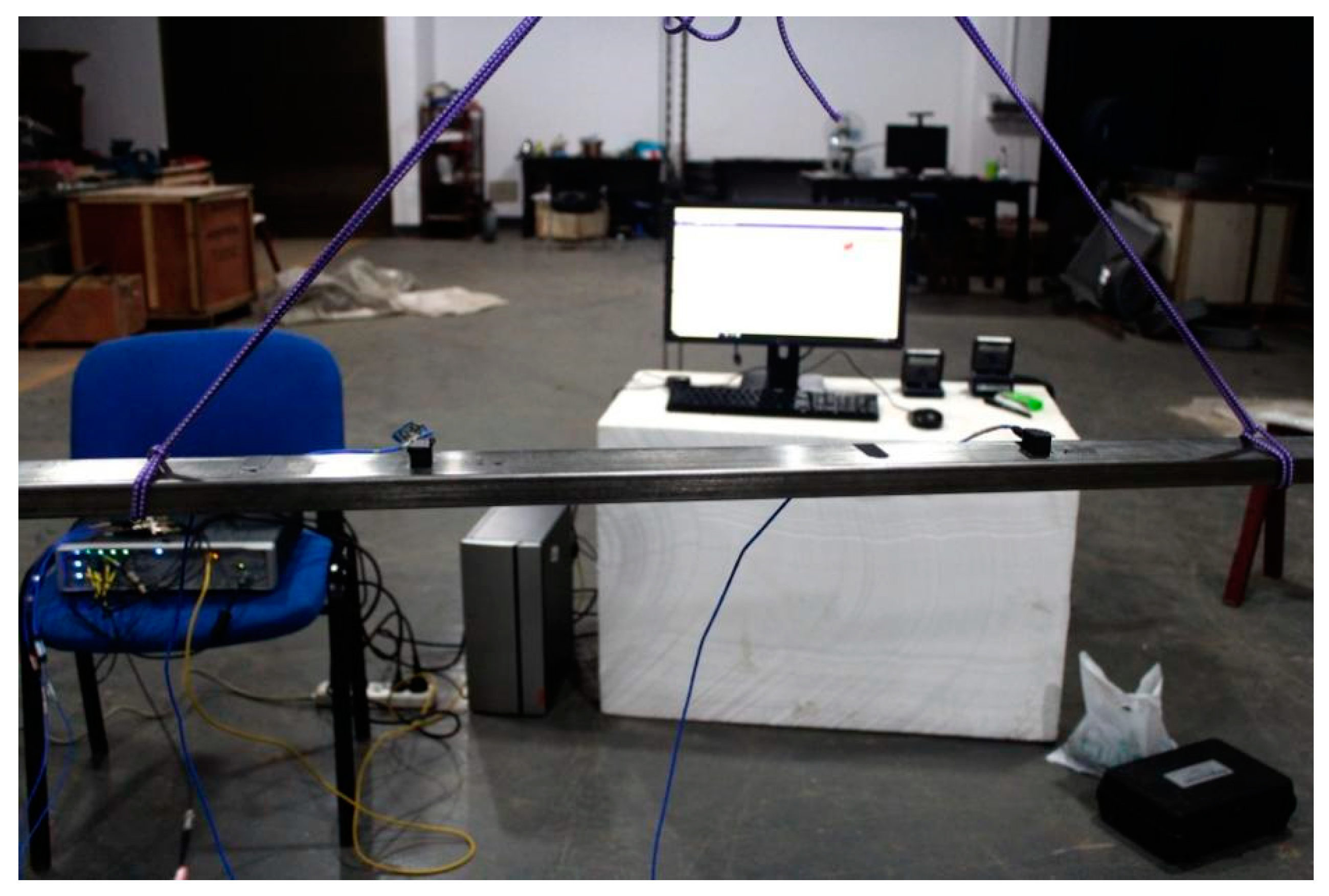
5.2. Experimental Setup and Instrumentation
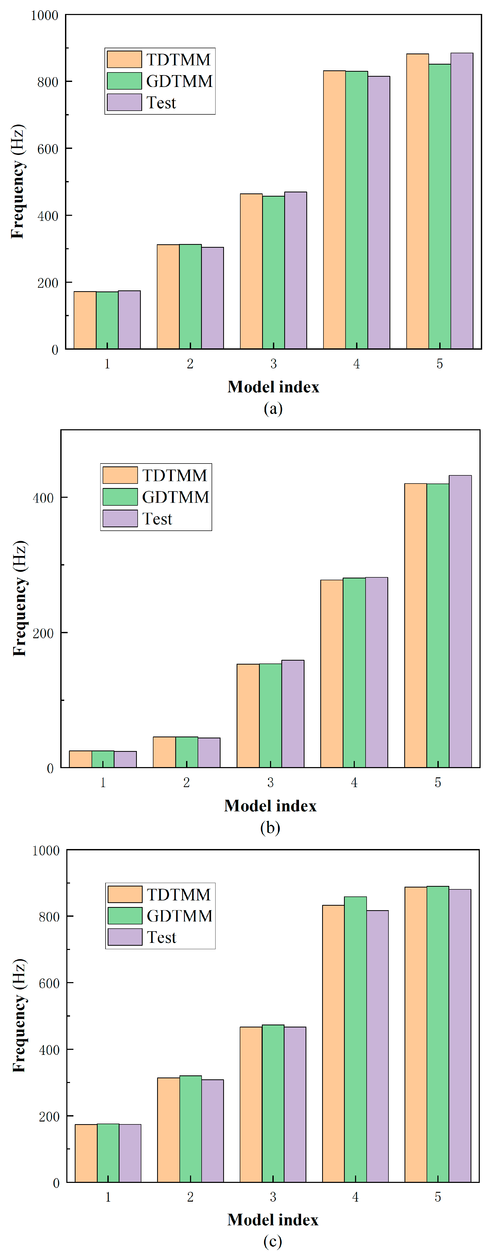
5.3. Dynamic Response
6. Conclusions
Author Contributions
Funding
Institutional Review Board Statement
Informed Consent Statement
Data Availability Statement
Conflicts of Interest
Appendix A
Appendix B
References
- Vlasov, V.Z. Thin-walled elastic beams. PST Cat. 1959, 428. [Google Scholar]
- Timoshenko, S.P. Theory of bending, torsion and buckling of thin-walled members of open cross section. J. Frankl. Inst. 1945, 239, 343–361. [Google Scholar] [CrossRef]
- Kim, Y.Y.; Kim, J.H. Thin-walled closed box beam element for static and dynamic analysis. Int. J. Numer. Methods Eng. 1999, 45, 473–490. [Google Scholar] [CrossRef]
- Song, O.; Librescu, L. Free vibration of anisotropic composite thin-walled beams of closed cross-section contour. J. Sound Vib. 1993, 167, 129–147. [Google Scholar] [CrossRef]
- Maalawi, K.Y. Dynamic Optimization of Functionally Graded Thin-Walled Box Beams. Int. J. Struct. Stab. Dyn. 2017, 17, 1750109. [Google Scholar] [CrossRef]
- Qin, H.; Liu, Z.; Liu, Y.; Zhong, H. An object-oriented MATLAB toolbox for automotive body conceptual design using distributed parallel optimization. Adv. Eng. Softw. 2017, 106, 19–32. [Google Scholar] [CrossRef]
- Yadav, A.; Panda, S.K.; Dey, T. Non-linear dynamic instability analysis of thin-walled stiffener beam subjected to uniform harmonic in-plane loading. J. Sound Vib. 2017, 408, 383–399. [Google Scholar] [CrossRef]
- Wu, Q.; Gao, H.; Zhang, Y.; Chen, L. Dynamical analysis of a thin-walled rectangular plate with preload force. J. Vibroengineering 2017, 19, 5735–5745. [Google Scholar] [CrossRef]
- Wang, B.; Zhou, Y.; Li, Y.; Hao, P.; Zhao, Y.; Wang, B. Free Vibration Analysis of Beam-Type Structures Based on Novel Reduced-Order Model. AIAA J. 2017, 55, 3143–3152. [Google Scholar] [CrossRef]
- Dokumaci, E. An exact solution for coupled bending and torsion vibrations of uniform beams having single cross-sectional symmetry. J. Sound Vib. 1987, 119, 443–449. [Google Scholar] [CrossRef]
- Bishop, R.; Cannon, S.; Miao, S. On coupled bending and torsional vibration of uniform beams. J. Sound Vib. 1989, 131, 457–464. [Google Scholar] [CrossRef]
- Laakso, A.; Romanoff, J.; Niemelä, A.; Remes, H.; Avi, E. Free vibration by length-scale separation and inertia-induced interaction–application to large thin-walled structures. Mech. Adv. Mater. Struct. 2022, 1–15. [Google Scholar] [CrossRef]
- Bebiano, R.; Eisenberger, M.; Camotim, D.; Gonçalves, R. GBT-Based Vibration Analysis Using the Exact Element Method. Int. J. Struct. Stab. Dyn. 2018, 18, 1850068. [Google Scholar] [CrossRef]
- Yaman, Y. Vibrations of open-section channels: A coupled flexural and torsional wave analysis. J. Sound Vib. 1997, 204, 131–158. [Google Scholar] [CrossRef]
- Arpaci, A.; Bozdag, S.; Sunbuloglu, E. Triply coupled vibrations of thin-walled open cross-section beams including rotary inertia effects. J. Sound Vib. 2003, 260, 889–900. [Google Scholar] [CrossRef]
- Ambrosini, D. On free vibration of nonsymmetrical thin-walled beams. Thin-Walled Struct. 2009, 47, 629–636. [Google Scholar] [CrossRef]
- Zhou, J.; Wen, S.; Li, F.; Zhu, Y. Coupled bending and torsional vibrations of non-uniform thin-walled beams by the transfer differential transform method and experiments. Thin-Walled Struct. 2018, 127, 373–388. [Google Scholar] [CrossRef]
- Kim, N.-I.; Fu, C.C.; Kim, M.-Y. Stiffness matrices for flexural–torsional/lateral buckling and vibration analysis of thin-walled beam. J. Sound Vib. 2007, 299, 739–756. [Google Scholar] [CrossRef]
- De Borbon, F.; Mirasso, A.; Ambrosini, D. A beam element for coupled torsional-flexural vibration of doubly unsymmetrical thin walled beams axially loaded. Comput. Struct. 2011, 89, 1406–1416. [Google Scholar] [CrossRef]
- Prokić, A.; Mandić, R.; Vojnić-Purčar, M. An improved analysis of free torsional vibration of axially loaded thin-walled beams with point-symmetric open cross-section. Appl. Math. Model. 2016, 40, 10199–10209. [Google Scholar] [CrossRef]
- Massonnet, C. A new approach (including shear lag) to elementary mechanics of materials. Int. J. Solids Struct. 1983, 19, 33–54. [Google Scholar] [CrossRef]
- Armanios, E.A.; Badir, A.M. Free vibration analysis of anisotropic thin-walled closed-section beams. AIAA J. 1995, 33, 1905–1910. [Google Scholar] [CrossRef]
- Kim, N.-I.; Lee, J. Improved formulation for spatial free vibration of thin-walled Al/Al2O3 FG sandwich beams with non-symmetric open, single- and double-cell sections. Compos. Struct. 2017, 178, 162–185. [Google Scholar] [CrossRef]
- Bastawrous, M.V.; El-Badawy, A.A. A Study on Coupled Bending and Torsional Vibrations of Wind Turbine Blades. Adv. Mater. Res. 2012, 622–623, 1236–1242. [Google Scholar]
- Tesar, A. The effect of diaphragms on distortion vibration of thin-walled box beams. Comput. Struct. 1998, 66, 499–507. [Google Scholar] [CrossRef]
- Kim, Y.Y.; Kim, Y. A one-dimensional theory of thin-walled curved rectangular box beams under torsion and out-of-plane bending. Int. J. Numer. Methods Eng. 2002, 53, 1675–1693. [Google Scholar] [CrossRef]
- Kenny, S.; Pegg, N.; Taheri, F. Dynamic elastic buckling of a slender beam with geometric imperfections subject to an axial impulse. Finite Elem. Anal. Des. 2000, 35, 227–246. [Google Scholar] [CrossRef]
- Li, J.; Shen, R.; Hua, H.; Jin, X. Coupled bending and torsional vibration of axially loaded thin-walled Timoshenko beams. Int. J. Mech. Sci. 2004, 46, 299–320. [Google Scholar] [CrossRef]
- Zhong, H.; Liu, Z.; Qin, H.; Liu, Y. Static analysis of thin-walled space frame structures with arbitrary closed cross-sections using transfer matrix method. Thin-Walled Struct. 2018, 123, 255–269. [Google Scholar] [CrossRef]
- Kollbrunner, C.F.; Hajdin, N. Stäbe Mit Undeformierbaren Querschnitten; Springer: Berlin/Heidelberg, Germany; New York, NY, USA, 2013. [Google Scholar] [CrossRef]
- Ewins, D.J. Modal Testing: Theory, Practice and Application; John Wiley & Sons: New York, NY, USA, 2009. [Google Scholar]
- Zhong, H.; Xu, T.; Yang, J.; Sun, M.; Gao, F. Optimization Design of Automotive Body Stiffness Using a Boundary Hybrid Genetic Algorithm. Machines 2022, 10, 1171. [Google Scholar] [CrossRef]


| Boundary Conditions | Completely Free | Fully Restrained | Partially Restrained |
|---|---|---|---|
| B | 0 | - | 0 |
| Ψ | - | 0 | - |
| Property | Example 1 |
|---|---|
| A (mm2) | 811.912 |
| Asy (mm2) | 527.428 |
| Asz (mm2) | 284.484 |
| Asyz (mm2) | −14.777 |
| Ssy (mm3) | 211.788 |
| Ssz (mm3) | −146.718 |
| IP (mm4) | 343,162.173 |
| IB (mm4) | 330,258.324 |
| Iw (mm6) | 1,550,049.125 |
| Is (mm4) | 6765.932 |
| Iy (mm4) | 155,654.904 |
| Iz (mm4) | 311,349.828 |
| ys (mm) | −0.249 |
| zs (mm) | 0.130 |
| ρ (kg/m3) | 7850 |
| Frequency Order | C-C | C-F | F-F | ||||||
|---|---|---|---|---|---|---|---|---|---|
| TDTMM | GDTMM | S-FEM | TDTMM | GDTMM | S-FEM | TDTMM | GDTMM | S-FEM | |
| 1 | 241.8 | 233.0 | 245.230 | 39.790 | 37.7688 | 39.838 | 245.5 | 210.2 | 250.675 |
| 2 | 340.1 | 376.3 | 345.6 | 56.2197 | 59.2963 | 56.289 | 344.8 | 423.1 | 352.747 |
| 3 | 650.4 | 688.1 | 646.102 | 241.7619 | 233.0407 | 243.847 | 648.4 | 637.1 | 669.766 |
| 4 | 910.0 | 993.9 | 907.428 | 340.0758 | 376.3319 | 343.314 | 904.8 | 1047.7 | 937.967 |
| 5 | 1212.6 | 1293.7 | 1195.276 | 650.4239 | 688.1152 | 657.997 | 1208.9 | 1336.8 | 1251.518 |
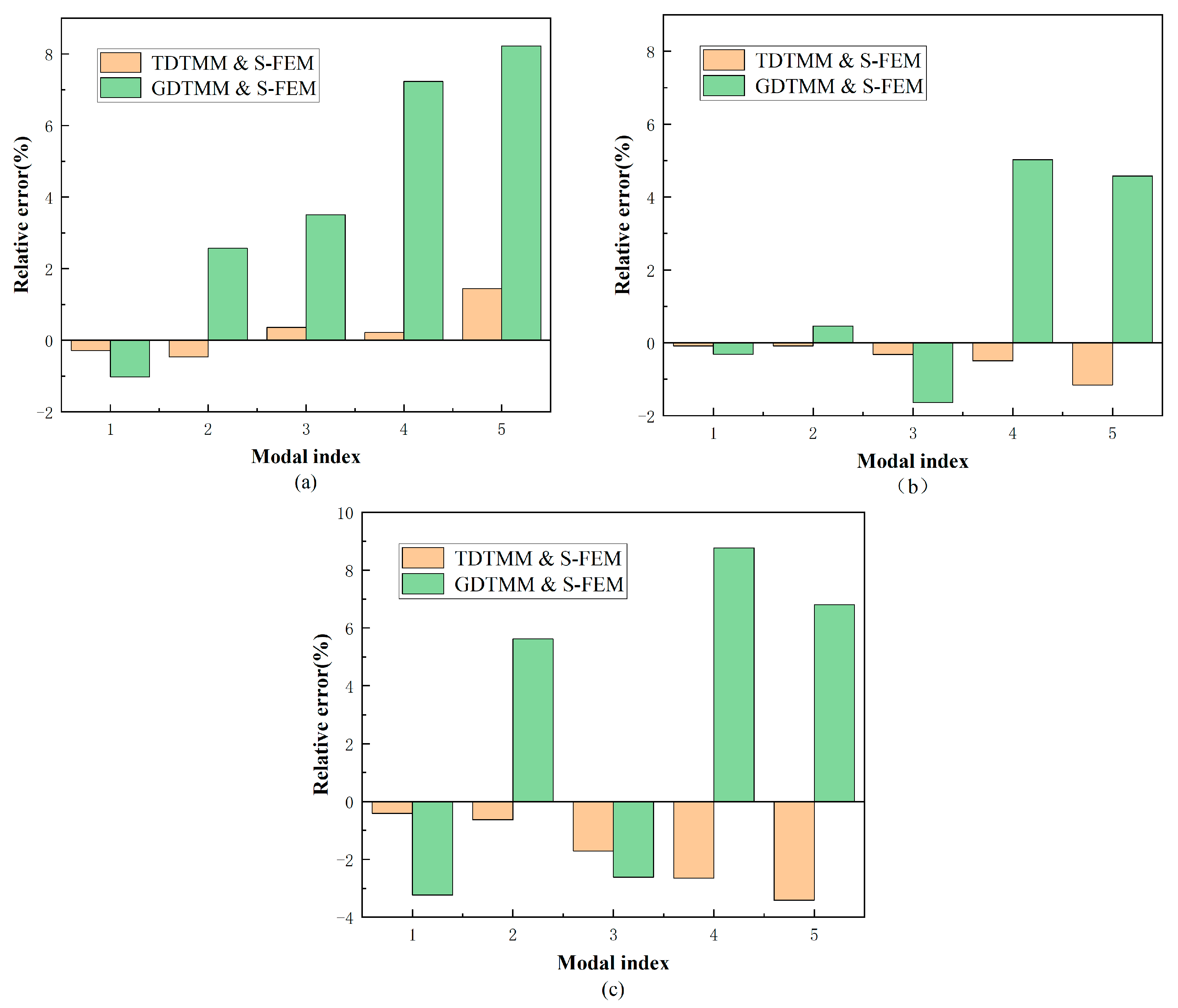
| Frequency Order | C-C (%) | C-F (%) | F-F (%) | |||
|---|---|---|---|---|---|---|
| TDTMM and FEM | GDTMM and FEM | TDTMM and FEM | GDTMM and FEM | TDTMM and FEM | GDTMM and FEM | |
| 1 | −0.29 | −1.02 | −0.01 | −0.31 | −0.41 | −3.23 |
| 2 | −0.46 | 2.57 | −0.01 | 0.46 | −0.63 | 5.62 |
| 3 | 0.36 | 3.51 | −0.32 | −1.64 | −1.71 | −2.61 |
| 4 | 0.22 | 7.23 | −0.49 | 5.02 | −2.65 | 8.77 |
| 5 | 1.45 | 8.23 | −1.15 | 4.58 | −3.41 | 6.81 |
| Property | Example 2 |
|---|---|
| A (mm2) | 480 |
| Asy (mm2) | 300 |
| Asz (mm2) | 180 |
| Asyz (mm2) | 0 |
| Ssy (mm3) | 0 |
| Ssz (mm3) | 0 |
| IP (mm4) | 180,000 |
| IB (mm4) | 168,750 |
| Iw (mm6) | 1,406,250 |
| Is (mm4) | 1440 |
| Iy (mm4) | 81,225 |
| Iz (mm4) | 175,135 |
| ys (mm) | 0 |
| zs (mm) | 0 |
| ρ (kg/m3) | 7850 |
| Frequency Order | C-C | C-F | F-F | ||||||
|---|---|---|---|---|---|---|---|---|---|
| TDTMM | GDTMM | S-FEM | TDTMM | GDTMM | S-FEM | TDTMM | GDTMM | S-FEM | |
| 1 | 231.1 | 233.7777 | 231.4303 | 37.5526 | 37.6162 | 37.5499 | 237.0261 | 234.3 | 236.4648 |
| 2 | 336.5 | 339.5076 | 338.3460 | 55.0734 | 55.1457 | 55.0781 | 345.7355 | 346.9 | 345.3933 |
| 3 | 629.4 | 646.0637 | 610.7315 | 231.0992 | 233.777 | 230.0915 | 638.2321 | 631.7 | 632.6028 |
| 4 | 907.6 | 802.3214 | 889.4257 | 336.5472 | 339.5076 | 336.1434 | 921.8177 | 932.6 | 919.5201 |
| 5 | 1187.7 | 1243.0 | 1131.682 | 629.3608 | 646.0637 | 621.7753 | 1210.4 | 1206.8 | 1183.521 |
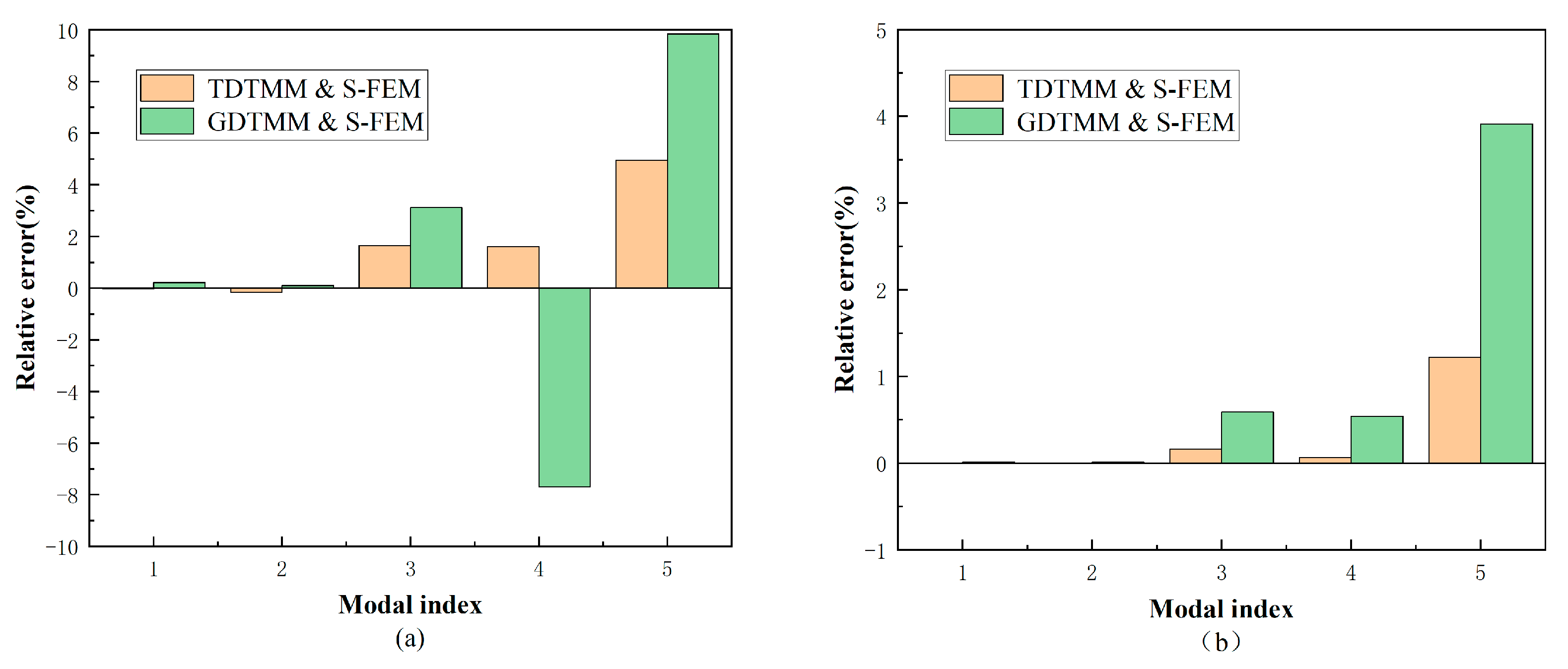
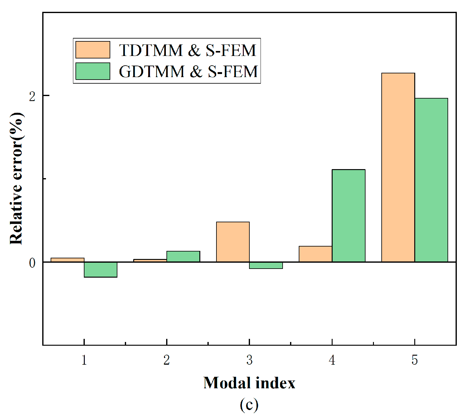
| Frequency Order | C-C (%) | C-F (%) | F-F (%) | |||
|---|---|---|---|---|---|---|
| TDTMM and S-FEM | GDTMM and S-FEM | TDTMM and S-FEM | GDTMM and S-FEM | TDTMM and S-FEM | GDTMM and S-FEM | |
| 1 | −0.03 | 0.21 | 0.0043 | 0.01 | 0.05 | −0.18 |
| 2 | −0.16 | 0.10 | −0.0076 | 0.01 | 0.03 | 0.13 |
| 3 | 1.65 | 3.12 | 0.16 | 0.59 | 0.48 | −0.08 |
| 4 | 1.61 | −7.7 | 0.06 | 0.54 | 0.19 | 1.11 |
| 5 | 4.95 | 9.84 | 1.22 | 3.91 | 2.27 | 1.97 |
| Property | Example 2 |
|---|---|
| A (mm2) | 204.739 |
| Asy (mm2) | 61.082 |
| Asz (mm2) | 143.657 |
| Asyz (mm2) | −1.780 |
| Ssy (mm3) | 41.304 |
| Ssz (mm3) | 40.761 |
| IP (mm4) | 52,964.834 |
| IB (mm4) | 46,093.812 |
| Iw (mm6) | 567,980.166 |
| Is (mm4) | 153.554 |
| Iy (mm4) | 62,444.724 |
| Iz (mm4) | 18,601.580 |
| ys (mm) | 0.465 |
| zs (mm) | 0.151 |
| ρ (kg/m3) | 7850 |
| Frequency Order | C-C | C-F | F-F | ||||||
|---|---|---|---|---|---|---|---|---|---|
| TDTMM | GDTMM | Test | TDTMM | GDTMM | Test | TDTMM | GDTMM | Test | |
| 1 | 172.19 | 171.27 | 173.96 | 24.85 | 24.89 | 24.20 | 173.62 | 175.73 | 174.50 |
| 2 | 312.23 | 312.43 | 304.40 | 45.43 | 45.56 | 44.13 | 313.97 | 320.16 | 308.24 |
| 3 | 463.60 | 456.44 | 469.14 | 153.29 | 153.77 | 159.12 | 466.86 | 473.28 | 467.05 |
| 4 | 831.56 | 830.19 | 814.93 | 277.92 | 280.35 | 281.56 | 832.80 | 858.59 | 816.79 |
| 5 | 882.49 | 851.94 | 885.07 | 420.30 | 420.06 | 432.56 | 887.73 | 889.98 | 880.48 |
| Frequency Order | C-C (%) | C-F (%) | F-F (%) | |||
|---|---|---|---|---|---|---|
| TDTMM and Test | S-FEM T- and Test | TDTMM and Test | S-FEM T- and Test | TDTMM and Test | S-FEM T- and Test | |
| 1 | −1.01 | −1.55 | −2.69 | 2.85 | −0.50 | 0.70 |
| 2 | 2.57 | 2.64 | 2.95 | 3.24 | 1.86 | 3.87 |
| 3 | −1.18 | −2.71 | −3.66 | −3.36 | −0.04 | 1.33 |
| 4 | 2.04 | 1.87 | −1.29 | −0.43 | −1.96 | 5.12 |
| 5 | −0.29 | −3.74 | −2.83 | −2.89 | 0.82 | 1.08 |
Disclaimer/Publisher’s Note: The statements, opinions and data contained in all publications are solely those of the individual author(s) and contributor(s) and not of MDPI and/or the editor(s). MDPI and/or the editor(s) disclaim responsibility for any injury to people or property resulting from any ideas, methods, instructions or products referred to in the content. |
© 2023 by the authors. Licensee MDPI, Basel, Switzerland. This article is an open access article distributed under the terms and conditions of the Creative Commons Attribution (CC BY) license (https://creativecommons.org/licenses/by/4.0/).
Share and Cite
Yang, J.; Xu, T.; Zhong, H.; Sun, M.; Gao, F. Experimental and Numerical Analysis of Triply Coupled Vibration of Thin-Walled Beam with Arbitrary Closed Cross-Section. Machines 2023, 11, 251. https://doi.org/10.3390/machines11020251
Yang J, Xu T, Zhong H, Sun M, Gao F. Experimental and Numerical Analysis of Triply Coupled Vibration of Thin-Walled Beam with Arbitrary Closed Cross-Section. Machines. 2023; 11(2):251. https://doi.org/10.3390/machines11020251
Chicago/Turabian StyleYang, Jianglin, Ting Xu, Haolong Zhong, Meng Sun, and Fei Gao. 2023. "Experimental and Numerical Analysis of Triply Coupled Vibration of Thin-Walled Beam with Arbitrary Closed Cross-Section" Machines 11, no. 2: 251. https://doi.org/10.3390/machines11020251