Article

Intelligent Road-Adaptive Semi-Active Suspension and Integrated Cruise Control †

1
Department of Control for Transportation and Vehicle Systems, Budapest University of Technology and Economics, Muegyetem rkp. 3, H-1111 Budapest, Hungary
2
Systems and Control Laboratory, Institute for Computer Science and Control (SZTAKI), Eötvös Loránd Research Network (ELKH), 13–17 Kende Street, H-1111 Budapest, Hungary
3
GIPSA-Lab, INPG, Université Grenoble Alpes, 11 Rue des Mathématiques, 38000 Grenoble, France
*
Author to whom correspondence should be addressed.
This paper is an extended version of our paper published in Basargan, H., Mihály, A., Gáspár, P., & Sename, O. (2022, June). Integrated adaptive velocity and semi-active suspension control for different road profiles. In 2022 30th Mediterranean Conference on Control and Automation (MED) (pp. 933–938). IEEE.
Machines 2023, 11(2), 204; https://doi.org/10.3390/machines11020204
Submission received: 14 December 2022 / Revised: 27 January 2023 / Accepted: 28 January 2023 / Published: 1 February 2023

Abstract

:
The availability of road and vehicle data enables the control of road vehicles to adapt for different road irregularities. Vision-based or stored road data inform the vehicle regarding the road ahead and surface conditions. Due to these abilities, the vehicle can be controlled efficiently to deal with different road irregularities in order to improve driving comfort and stability performances. The present paper proposes an integration method for an intelligent, road-adaptive, semi-active suspension control and cruise control system. The road-adaptive, semi-active suspension controller is designed through the linear parameter-varying (LPV) method, and road adaptation is performed with a road adaptivity algorithm that considers road irregularities and vehicle velocity. The road adaptivity algorithm calculates a dedicated scheduling variable that modifies the operating mode of the LPV controller. This modification of operation mode provides a trade-off between driving comfort and vehicle stability performances. Regarding the cruise control, the velocity design of the vehicle is based on the ISO 2631-1 standard, the created database, and the look-ahead road information. For each road irregularity, the velocity of the vehicle is designed according to previous measurements and the table of ISO 2631-1 standard. The comfort level must be selected in order to calculate dedicated velocity for road irregularity. The designed velocity is tracked by the velocity-tracking controller evaluated with the LPV control framework. The designed controllers are integrated, and the operation of the integrated method is validated in a TruckSim simulation environment.

1. Introduction

The chassis control of road vehicles is a hot topic in both industry and academia. There are several important criteria for vehicles, including driving comfort, vehicle safety, and stability. For this reason, vertical dynamics control has an important role in vehicle technology, where vertical control is performed by controlling the vehicle’s suspension system. The fundamental of a vehicle suspension system is to isolate the vehicle from road irregularities in order to improve road holding and driving comfort characteristics [1]. It consists of three main elements, which are an elastic element, the damping element, and several mechanical elements. The elastic element delivers a force to the suspension while it carries the whole static load. This element is typically a coil spring. The damping element is usually a shock absorber that delivers a dissipative force to the elongation speed. The mechanical element group links the sprung body to the unsprung mass [2].
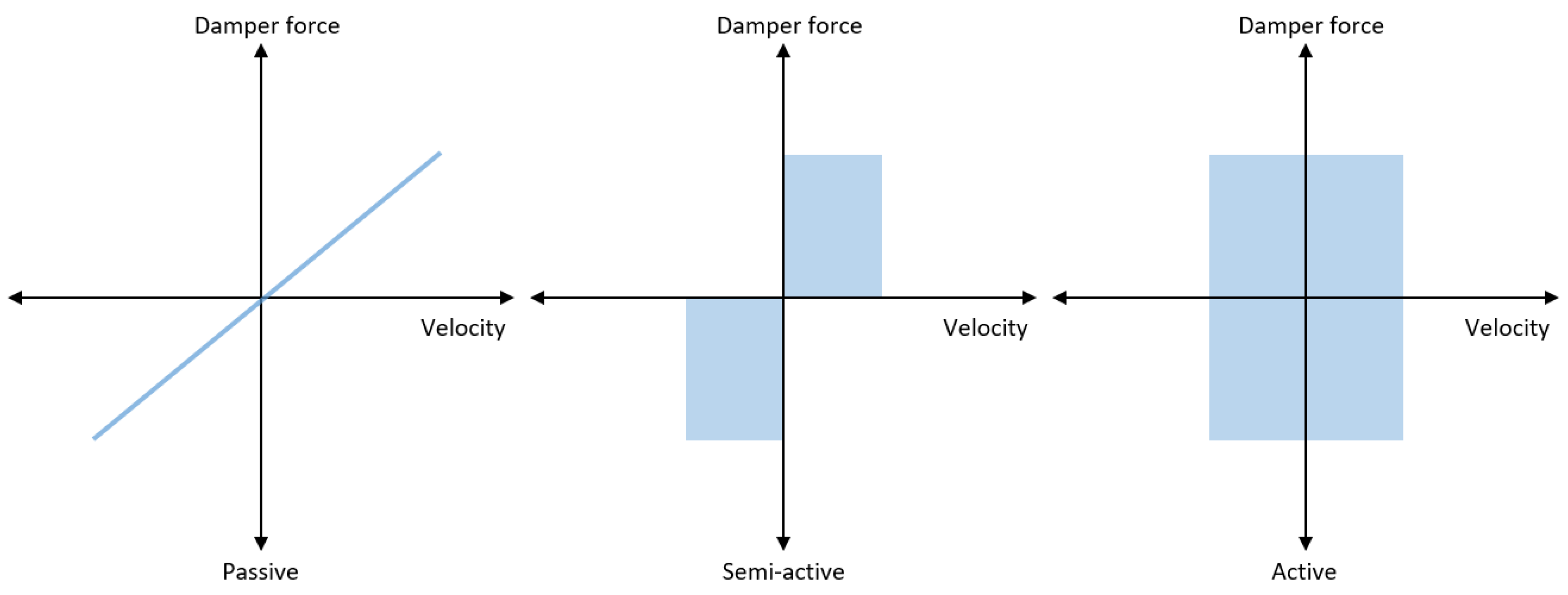
The suspension systems can be classified into three main categories: passive, active, and semi-active suspension. This classification depends on the damper force vs. damper velocity diagram, which is shown in Figure 1. Semi-active suspension has great potential in the automotive market due to its advantages compared to active and passive suspensions, such as negligible power demand, improvement in vehicle performance, safety features, and low weight and costs [2,3]. Thus, semi-active suspension is studied in this paper. The limitation of passive suspensions to improve the driving comfort and road holding together has motivated the development of controlled suspension systems, both active and semi-activeControlled suspension systems are developed due to the lack of improvement in both driving comfort and road holding together [4].
The primary problem of the vehicle suspension design is to deal with conflicting demands, such as high driving comfort, good road-holding features, and low suspension working space [4]. In order to ensure good driving quality, the vehicle must be isolated from road disturbances and irregularities. The vertical acceleration of the vehicle quantifies the driving quality. Furthermore, ensuring road-holding performance is realized by considering the tire loads [1]. Moreover, optimal driving comfort and road-holding performance should be ensured while considering the allowable suspension working space of the vehicle [5].
Due to the high availability of measurement data of vehicles, the performances of future vehicles can be improved. There are several different road conditions and irregularities which need to be considered during the design. Thus, the vehicle must be adaptive to different road conditions and irregularities, in addition to altering velocities, in order to ensure vertical and longitudinal comfort and road holding. For this reason, vertical control is a key point in order to achieve road-holding performance with different road irregularities, and the integration of the longitudinal dynamics of the vehicle into the vertical control can also ensure driving comfort. The longitudinal dynamics of the vehicle affect the vertical dynamics significantly, which can be observed by analyzing several data and simulations where it was shown that the velocity of the vehicle changes the vertical dynamics dramatically. Therefore, an online, reconfigurable, adaptive, semi-active suspension controller must be designed in order to ensure the road adaptivity of the vehicle. At the same time, the cruise controller must also be designed and integrated into the semi-active suspension control to ensure driving comfort and road-holding performance of the vehicle.
There are several control methods that deal with semi-active suspension control in the literature, such as Skyhook [6,7], linear-quadratic control [8,9], model predictive control [10,11], and H control [12,13]. However, the real-time configuration is not possible with the mentioned control methods. Due to the LPV framework, the controller can be reconfigured online by changing a scheduling variable [14,15]. Thus, the LPV framework has been used in this study.
Most of the adaptive preview control methods found in the literature, and in industry practice as well, rely on camera-based road assessment, as detailed in [16]. In that paper, adaptive Skyhook suspension was presented to adjust the vertical damping force of the suspension in real time using machine-vision-based road data, showing great improvement over speed bumps. In order to avoid the additional cost of a camera-based system and to gain information of various road distortions, some recent studies focused on exploiting the possibilities using novel vehicle–cloud–vehicle (V2C2V) communication. For instance, in [17], a method was proposed that uses cloud computing techniques to improve the ride quality of the vehicle by selecting different damping modes for the semi-active suspension based on the forthcoming road profile. A comprehensive analysis of preview-based techniques for vehicle suspension control has been performed; see [18].
The method in this paper has an advantage over previous methods by integrating cruise control in the semi-active control process. Thanks to the LPV framework, the controller can be reconfigured online by changing a scheduling variable [14,15]. For this reason, the LPV framework was used in this study. Although some previous research [19] has already aimed at integrating the longitudinal and vertical dynamics control in an LPV framework, the present paper deals with different types of road irregularities, focusing on more challenging road bumps and sine-sweep distortions.
A detailed literature review showed that the earlier proposed systems do not focus on the online reconfigurable road adaptivity by considering the cruise control and vehicle velocity for different road irregularities. Due to this research gap and problem, the new online, reconfigurable, adaptive, semi-active suspension controller must be integrated into the look-ahead cruise control, where the road adaptivity is ensured with the adaptivity method.
This paper is an extended version of the Mediterranean Conference on Control and Automation (MED) 2022 article [20]. The novelties of the paper are the integration of velocity designer and tracing control as a cruise controller and the performed extended simulation of the proposed method. The database design is also introduced in this paper, which was not in the previous paper, and an introduction section is provided.
This paper proposes a cruise control system. The design is based on the ISO 2631-1 standard, and the velocity is tracked with the proposed velocity-tracking controller that was designed through an LPV framework. The adaptive semi-active suspension controller was designed through the LPV method, where the scheduling variable enables one to perform a trade-off between vehicle performances, which are vehicle stability and driving comfort. Integration of these controllers makes the system intelligent and road-adaptive. The integration was performed with a sensitive adaptivity algorithm that is based on the designed database.
The article is organized as follows: Section 2 presents the modeling of the quarter-car suspension and LPV control synthesis of the adaptive semi-active suspension control. Section 3 introduces the cruise control system, where Section 3.1 presents the velocity design based on the ISO 2631-1 standard and Section 3.2 proposes a velocity-tracking controller through the LPV method. The road adaptivity algorithm, database design, and system integration are shown in Section 4. The operation of the proposed method is demonstrated and validated in Section 5, which was achieved in a TruckSim environment by integrating real road data. Finally, concluding remarks are presented in Section 7.

2. Semi-Active Suspension Controller Design

In this section, the design of a semi-active suspension controller is introduced. This design has already been proposed in [
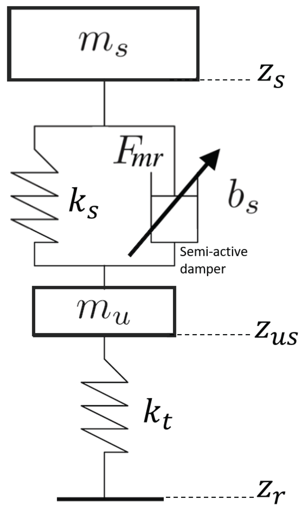
20], which is the basis of the design in this study. The widely used control-oriented quarter-car model is applied in this study; the model is shown in Figure 2. The dynamics of the actuator and semi-active suspension are described in Equations (1) and (2).
m s z s ¨ + b s ( z s ˙ z u s ˙ ) + k s ( z s z u s ) + F m r = 0 m u z u s ¨ + b s ( z u s ˙ z s ˙ ) + k s ( z u s z r ) + k s ( z u s z s ) F m r = 0
F ˙ m r = 1 τ F m r + 1 τ u
Here, sprung mass and unsprung mass are expressed by m s and m u , and the tire and spring vertical stiffness are described as k t and k s . The time constant and shock absorber damping rate are represented as τ and b s , respectively. Vertical displacements of unsprung mass and sprung mass are expressed by z u s and z s ; the road disturbance derived from road irregularities is represented as z r . The control input u is F, and the damper force generated by the actuator is F m r . The relationship between the damper force generated by the actuator and control input is presented in (2). Table 1 shows the parameters of the suspension model.
Figure 2. Control-oriented quarter-car model.
Machines 11 00204 g002
The components of the state vector x = x 1 x 2 x 3 x 4 x 5 T are shown in The state vector x is selected as x = x 1 x 2 x 3 x 4 x 5 T ; see Equation (3).
x 1 = z s x 2 = z u s x 3 = z s ˙ x 4 = z u s ˙ x 5 = F m r
Next, the state-space representation form must be written from the system given with Equation (1) as follows:
x ˙ = A x + B 1 w + B 2 u
z = C 1 x + D 11 w + D 12 u
y = C 2 x + D 21 w + D 22 u
Equation (1) is arranged to find matrices according to the measured signal, performance vector components, and state-vector components. Depending on Equation (Section 2), the results are arranged, and the coefficients of the x , w , u are computed. The computed coefficients give the matrices for the control design.
The unmodelled dynamics Δ ( Δ < 1 ) are presented as follows: Δ ( ω 1 ) = 0.25 at low frequencies and Δ ( ω 2 ) = 1 at high frequencies.
The performance specifications are defined to achieve a trade-off between vehicle stability and driving control, and damper force must also be minimized. The first goal is enhancing the driving comfort by defining the following performance criterion: z 1 = z s ¨ 0 . Here, the vertical acceleration of the sprung mass is minimized. The second goal is ensuring roll and pitch stability of the vehicle by minimizing the suspension deflection, z 1 = z s ¨ 0 . The third goal is the minimization of tire deformation by the following criterion: z 3 = ( z u s w ) 0 . This goal enhances the road holding of the vehicle. The last goal is minimizing the damper force, z 4 = F 0 . All the goals are put in a performance vector z = z 1 z 2 z 3 z 4 T .
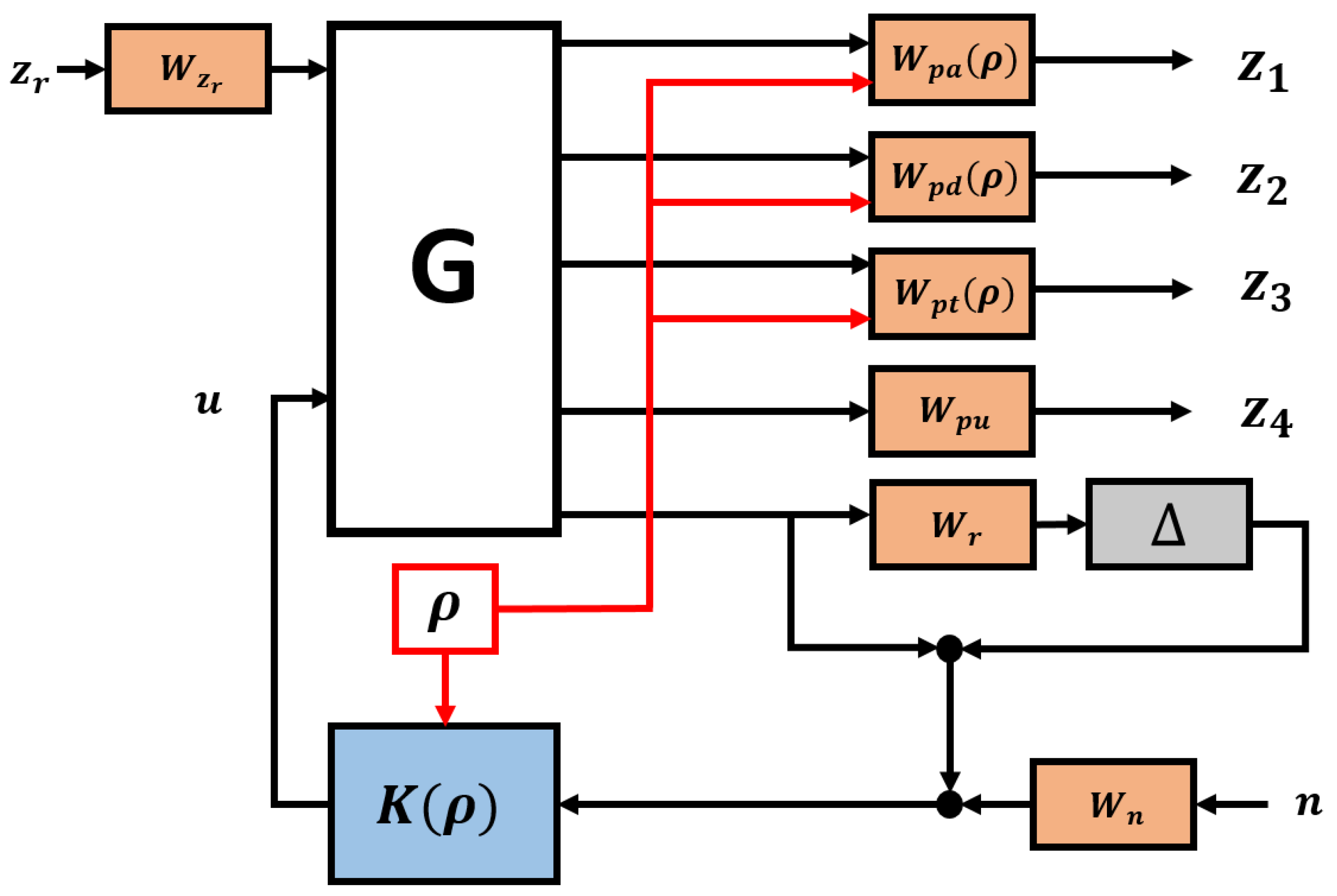
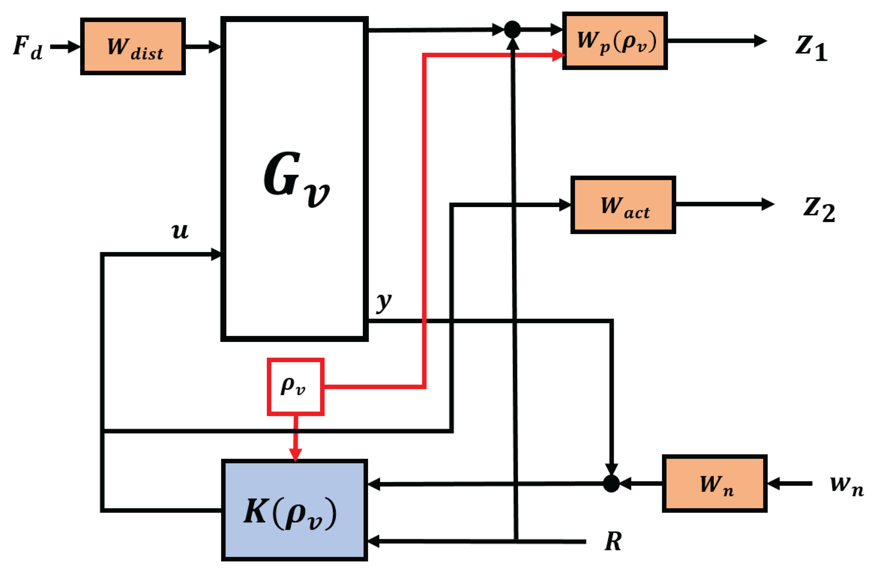
Figure 3 shows a closed-loop architecture with a weighting strategy, where G is quarter-car, K is a designed semi-active suspension controller that is characterized by scheduling variable ρ , z r is road disturbance, and y = q 1 q 2 is measured output.
The uncertainties of the vehicle model are considered by Δ and the W r weighting function. Road disturbances and vehicle performances are represented by weighting functions W z r and W p .
Performance weighting functions aim to keep the tire deflection ( W p t ), suspension deflection ( W p d ), control input ( W p u ), and sprung mass acceleration ( W p a ) small over the required frequency range. The driving comfort is expressed by W p a , and the road holding and safety performance of the vehicle are represented by W p d and W p t .
The performance weighting functions are designed by ensuring the trade-off between performances. The scheduling variable ρ   [ 0.01 , 0.99 ] is characterized the weighting functions W p t , W p a , and W p d in order to specify the significance of one of the performances for the incoming road conditions. The weighting functions are given as follows:
W p a = ρ α 1 s + 1 T 1 s + 1
W p d = ( 1 ρ ) α 2 s + 1 T 2 s + 1
W p t = ( 1 ρ ) α 3 s + 1 T 3 s + 1
where T 1 , 2 , 3 and α 1 , 2 , 3 are designed parameters. The other weighting functions do not contain scheduling variables, and they are of a linear form.
An LPV controller has been designed in a manner such that closed-loop quadratic stability is ensured, while at the same time the induced L 2 norm from the disturbance ω to the performance vector z is smaller than the value γ ; see [21]. Hence, the disturbance attenuation problem is formalized as follows:
inf K sup ϱ F P sup w 2 0 , w L 2 z 2 w 2 γ
The solution of the parameter-varying control design problem is governed by the set of infinite-dimensional LMIs which is satisfied for all ρ F P ; thus, the problem is convex. The LPV problem is arranged by gridding the parameter space, then solving the set of linear matrix inequalities that hold for the subset of F P , as detailed in [22]. The controller that settles the LPV γ -performance problem can be specified as the feasibility of a set of the linear matrix inequalities that can be solved numerically. The closed-loop system is exponentially stable, if there is an X ( ρ ) > 0 satisfying the following LMIs for all ρ , where x T X ( ρ ) x is a parameter-dependent Lyapunov function for the closed-loop system; see [23].
A c l T X + X A c l T + d / d t ( X ) X C c l γ 1 C T B c l T X I γ 1 D c l T γ 1 C c l γ 1 D c l I .
In the designed reconfigurable LPV controller, ρ = 0.01 stands, where the road holding and stability performance of the vehicle are preferred, whereas the driving comfort is considered by ρ = 0.99 . The combination of performance is ensured if the scheduling variable is between the edge values.

3. Integrated Cruise Control Design

This section describes the integrated cruise control, where the velocity design is based on the ISO 2631-1 standard and the tracking controller was designed through the LPV method.

3.1. Velocity Design

Velocity design is a key objective for improving driving comfort and road-holding performances for vehicles. In order to improve vehicle performance, the velocity of the vehicle must differ for different road irregularities. Vehicles should not be operated at high velocities over challenging road irregularities, as they can cause physical harm to the vehicle chassis and affects passenger comfort. For this reason, the velocity must be designed based on the road information in order to increase vehicle performance.
In this study, four road irregularities were used in order to validate the proposed method. These road irregularities are called road profiles in this study. These road irregularities are shown in Figure 4. The road profiles are listed below:
  • Road I: Sine-sweep road irregularity.
  • Road II: 10 cm bumps irregularity.
  • Road III: Several bumps.
  • Road IV: 5 cm bump.
Figure 4. Road irregularities.
Machines 11 00204 g004
The database was designed with several simulations, where different road profiles and vehicle velocities were simulated. The scheduling variable ρ was selected to be 0.01 due to considering the worst-case scenario to ensure vehicle stability. Please note that ρ = 0.01 stands for road holding or vehicle stability performance. Part of the simulation results are listed in Table 2 and Figure 5, whose data were interpolated into the database. The root mean square (RMS) value of each velocity was stored in the database. Please note that these data are different from the data that were used in order to design the scheduling variable that ensures road adaptivity.
The filter (7) was applied to the sprung mass acceleration in order to characterize human comfort [24].
W I S O ( s ) = 81.89 s 3 + 796.6 s 2 + 1937 s + 0.1446 s 4 + 80 s 3 + 2264 s 2 + 7172 s + 21196
The comfort-oriented driving analysis can be performed with the ISO 2631-1 standard for different road profiles and velocities. Table 3 shows frequency-weighted vibration magnitude (FWVM) and its likely changes in public transportation. The FWVM value is calculated by Equation (13). Acceptable values of vibration magnitude for comfort depend on many factors, which vary with each application. These FWVM values give approximate indications of likely reactions to various magnitudes of overall vibration total values in transport. The reactions depend on a passengers’ expectations regarding the duration of the trip, the types of activities expected to be accomplished by passengers, etc. [25].
In Table 2, the comfort level was selected to be below “uncomfortable” for public transport. For this reason, the comfort limit was 1.6 m/s 2 , and below this limit, the velocity for dedicated road irregularity was calculated according to the database. The velocity and vertical acceleration RMS values were stored in the database under the selected comfort limit, and the maximum interpolated velocity was selected as a designed velocity.
The vehicle velocity must be feasible, which means that if the speed limit of the road is 70 km/h, then the vehicle cannot decelerate instantly to 20 km/h. Thus, this feasibility must also be considered in the design of velocity and selection of the comfort limit. The designed velocities are listed in Table 4. Please note that the calculated velocity was 76.42 km/h for road IV, but due to the 70 km/h speed limit, a dedicated velocity was selected as the velocity limit value.

3.2. Velocity Controller Design

The longitudinal dynamics of the vehicle are introduced and the design of the velocity-tracking controller is explained in this section.
First, the longitudinal dynamics of the vehicle are formulated for designing the velocity-tracking controller:
m ξ ¨ = F l F d
where the mass of the vehicle is expressed as m, and ξ is the displacement. Longitudinal force is presented as F l , and disturbance force is presented as F d .
The definition of disturbance force is the sum of the drag disturbance, rolling disturbance, and road slope disturbance: F d = F d 1 + F d 2 + F d 3 . The drag disturbances depend on the frontal area of the vehicle A F , drag coefficient C d , wind velocity w, velocity ξ ˙ , and air density ϱ . The wind velocity is negative for a tailwind and positive for a headwind.
F d 1 = 0.5 C d ϱ A F ( ξ ˙ + w ) 2
A rolling resistance is the function of road surface coefficient f, vehicle mass, and road slope angle α :
F d 2 = m g f c o s ( α )
The disturbance hailing from the road slope:
F d 3 = m g s i n ( α )
For the next step, the longitudinal motion equation of vehicle (8) must be transformed into the state-space representation form that is shown in (12).
x ˙ = 0 1 0 0 x + 0 1 m w + 0 1 m u y = 0 1 x
The state vector x = [ ξ , ξ ˙ ] T contains the longitudinal velocity and displacement. The control input of the system is longitudinal force u = F l , and the measured output of the system is the velocity of vehicle y = ξ ˙ . The disturbance of the system is w = F d .
Following the reference velocity is the first task of the vehicle. This criterion is formalized as follows: z 1 = [ ξ ˙ r e f ξ ˙ ] , where the optimization criterion: z 1 0 . Moreover, actuator saturation must also be avoided. The maximal forces of the braking and driveline systems are determined by their physical construction limits. The consideration of these limits is also necessary with the following formulation: z 2 = F l .
Figure 6 shows the velocity-tracking controller that is founded on a weighting strategy formulated through a closed-loop architecture. Here, the longitudinal vehicle model is expressed as G v , and K is the designed LPV controller characterized with ρ v e l , which is responsible for control reconfiguration. The measurement noise, performance output, and control input of the actuator are represented as n, z, and u, respectively. The role of the scheduling variable in this controller aims to configure the sensitivity of velocity tracking, and it is used as the constant ρ v = 1 in this study. The weighting function of disturbance and sensor noises are expressed by W d i s t and W n , respectively. The weighting function for the actuator is W a c t , and performance criteria are represented with W p .

4. Road Adaptivity and System Integration

In this section, the road adaptability algorithm is proposed with the integration of the system. First, database design is introduced briefly, and then scheduling variable design is explained. Finally, system integration is proposed with all controllers and adaptivity methods.

4.1. Database Design

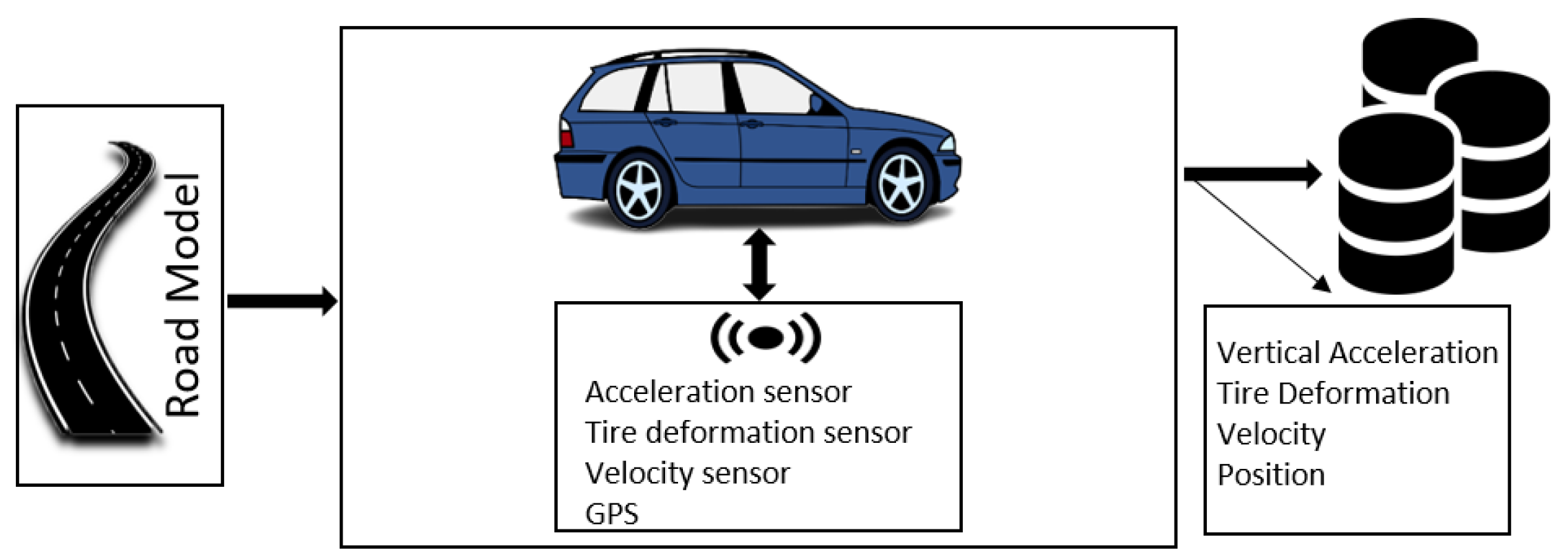
The previous measurements or available data related to vehicle dynamics and road conditions have a significant role in the study in order to propose the adaptivity method for the integration of velocity and adaptive semi-active suspension control. These measurements or available data must be stored in a database to use at a dedicated time. For this reason, the database has been designed to use with the adaptivity method. In this study, the detection or estimation of road model and irregularity is not in the focus; thus, the position information of road irregularities is stored in the database. The data collection architecture is shown in Figure 7.
The data are collected by the onboard unit of the vehicle with multiple sensors (GPS, acceleration, tire deformation, velocity). The collected data are listed below, and these collected data are gathered and stored in a database:
  • Vertical acceleration;
  • Tire deformation;
  • Velocity;
  • Position.
Several sensors are used for measurement: acceleration sensor, tire deformation sensor, velocity sensor, and GPS. A tire deformation sensor is not common or easily accessible, and there are several methods and studies to design the sensor that measures the tire deformation [26,27].
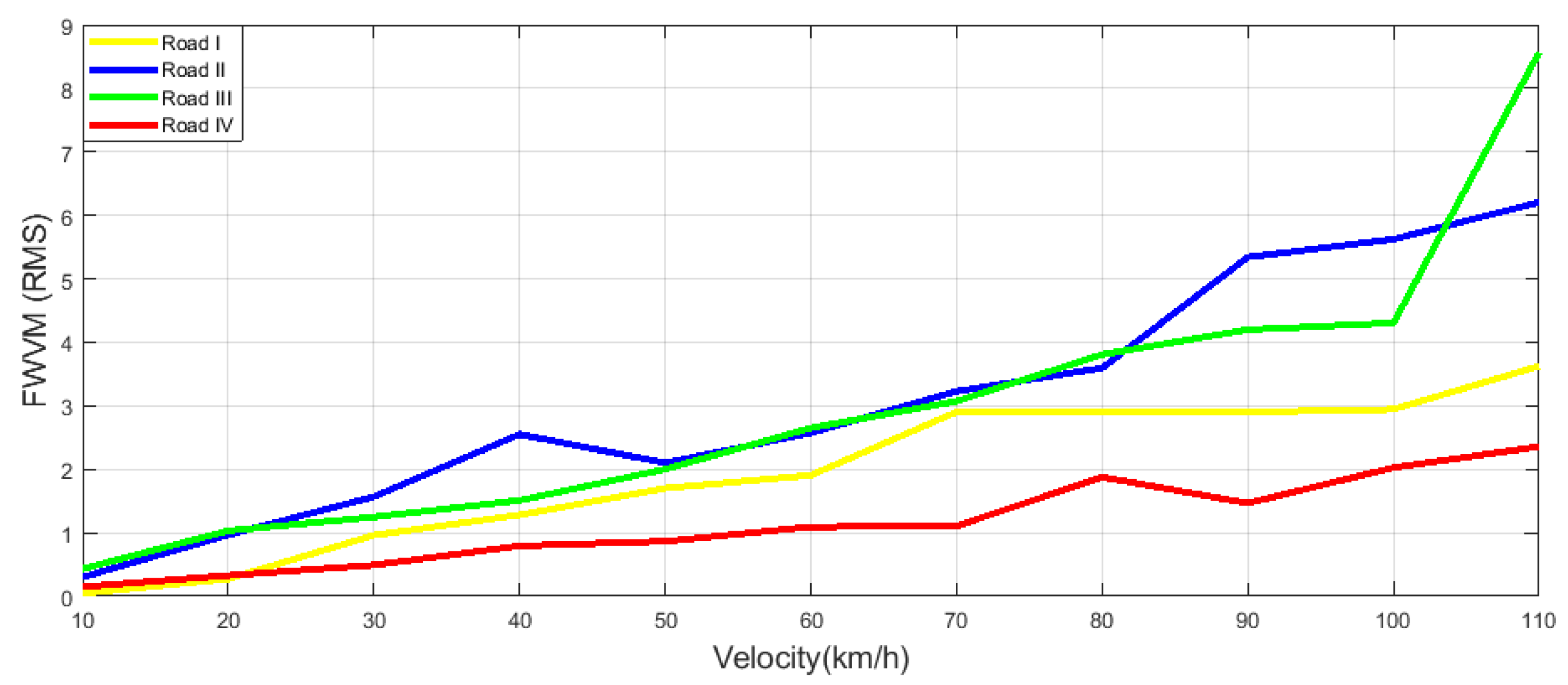
The calculations of the root mean square (RMS) values of performances are found below:
P v a = 1 T a 0 T a a 2 ( t ) d t P t d = 1 T t 0 T t t d 2 ( t ) d t
where a ( t ) and t d ( t ) are time-weighted acceleration and tire deformation, respectively; and T t and T a are the numbers of tire deformation and acceleration values.
The normalized vertical acceleration and tire deformation values are calculated as follows:
ζ i , j k = P i , j k P m a x k
where ζ is the normalized value; the RMS of the performance is P ; k [ v a , t d ] , where t d is the tire deformation and v a is the vertical acceleration performance; i is the road type; j is the velocity of the vehicle.

4.2. Scheduling Variable Design

The scheduling variable can be changed in real time, and thanks to the LPV method, the controller’s behavior can be modified by changing this variable. The road adaptivity is performed by designing the scheduling variable for each velocity and road irregularity.
The scheduling variable is designed in two steps. In the first step, performance index Υ is found. The second step contains the calculation of a shifting index κ depending on κ and Υ ; a scheduling variable ρ is found.
In the first step, it is necessary to compare performance results in the road profile and the corresponding velocity in the database. For this reason, the normalized value of RMS values of vertical acceleration and tire deformation was calculated and stored in a database.
The comparison of these normalized values gives importance to one of these performances. In the case of the normalized value of tire deformation, ζ t d is greater than the normalized value of vertical acceleration ζ v a , the focus should be tire deformation, and this performance must be minimized by choosing Υ = 0 . In the case of the normalized value of vertical acceleration ζ v a being greater than the normalized value of tire deformation ζ t d , the focus should be vertical acceleration, and this performance must be minimized by choosing Υ = 1 . If the normalized values are equal each other, then Υ is selected as 0.5. The selection procedure of the performance index is shown in (15).
Υ = 0 , if ζ t d > ζ v a 1 , if ζ t d < ζ v a 0.5 , if ζ t d = ζ v a
The shifting index describes the distance of the scheduling variable from its middle range, which is 0.5. In the next step, shifting index κ is found according to the rate index χ that is calculated by the average rate between the normalized value of tire deformation and vertical acceleration in the database, and it was taken as two according to data in the database. The reason for the selection of the rate index as two is that if the rate of the corresponding normalized performance value is greater than two, κ is 0.5 . Here, κ cannot be greater than 0.5 because of limitation of scheduling variable ( ρ [ 0.01 , 0.99 ] ). The calculation of the shifting index is shown in Equation (16).
κ = 0.5 , if ζ t d ζ v a ζ v a ζ t d > = χ ζ t d ζ v a 0.25 , if ζ t d > ζ v a ζ v a ζ t d 0.25 , if ζ v a > ζ t d
Finally, the scheduling variable is calculated based on the results of vehicle’s performance in the corresponding velocity and road profiles, performance index, and shifting index. It is handled by Equation (17).
ρ = 0.5 κ , if Υ = 0 0.5 + κ , if Υ = 1 0.5 , if Υ = 0.5

4.3. System Integration

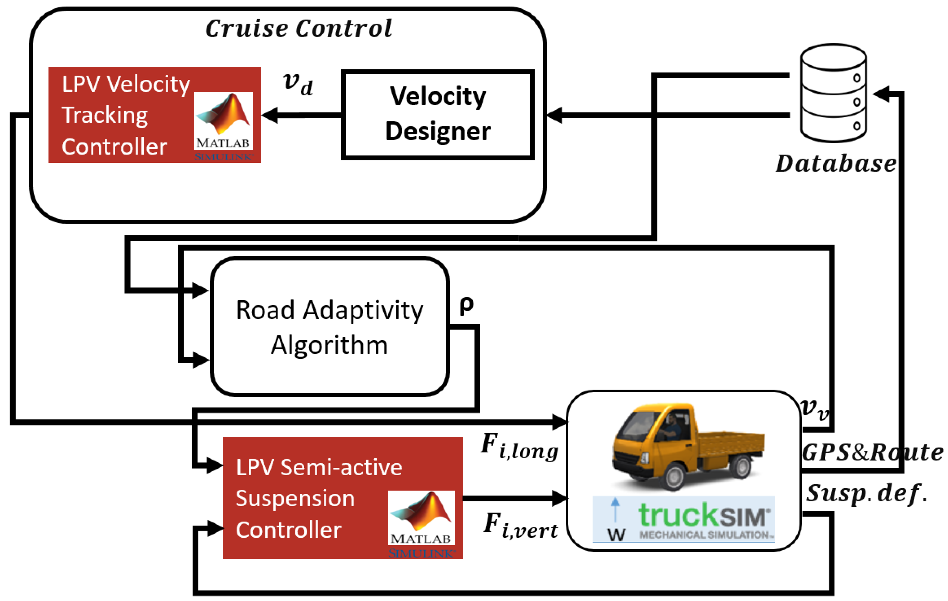
The system’s architecture is depicted in Figure 8. The velocity-tracking controller and semi-active suspension controller were designed and integrated into Simulink. The TruckSim simulation environment was integrated into Simulink. Velocity, GPS, route, and suspension deflection of the vehicle were gathered from TruckSim to Simulink. The GPS&Route information was stored in a database, and this database was used in cruise control and for the road adaptivity algorithm. Velocity was designed with look-ahead road information, and designed velocity was tracked by an LPV velocity-tracking controller. It calculates the longitudinal force for each tire. The road adaptivity algorithm finds the dedicated scheduling variable for each velocity and road irregularity. The semi-active suspension controller calculates the vertical damper forces for each corner of the vehicle by using scheduling variables and measured output suspension deflection.

5. Simulation Results and Analysis

For simulation purposes, a compact utility truck was selected due to its independent front and rear semi-active suspension. Note that for heavy duty trucks having rigid front and rear axles or multiple wheel setups, the proposed quarter car-based controller design is not applicable. With the modification of the baseline vehicle model, it is possible to design a semi-active damper controller with a similar method considering road disturbances and velocity; however, due to the significantly changing payload, comfort requirements are generally met by the use of seat suspension systems [28].
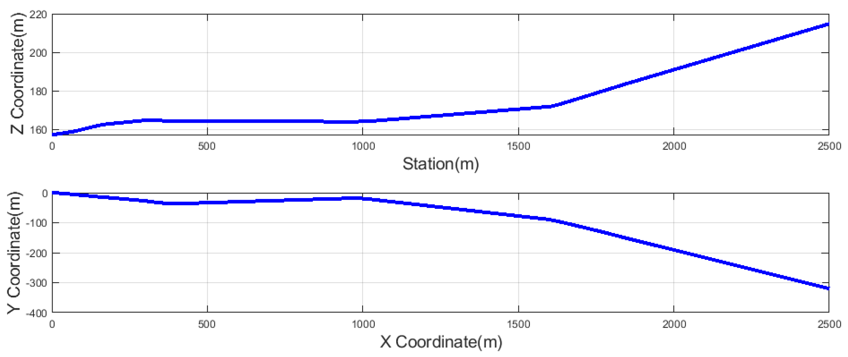
The simulation route is the Hungarian highway (Gyöngyös–Kápolna) based on real geographical data; see Figure 9. The simulation rouse was implemented in a TruckSim environment. The speed limit of the simulation route was 70 km/h. The designed velocity, designed scheduling variable, road irregularities, and their locations are shown in 
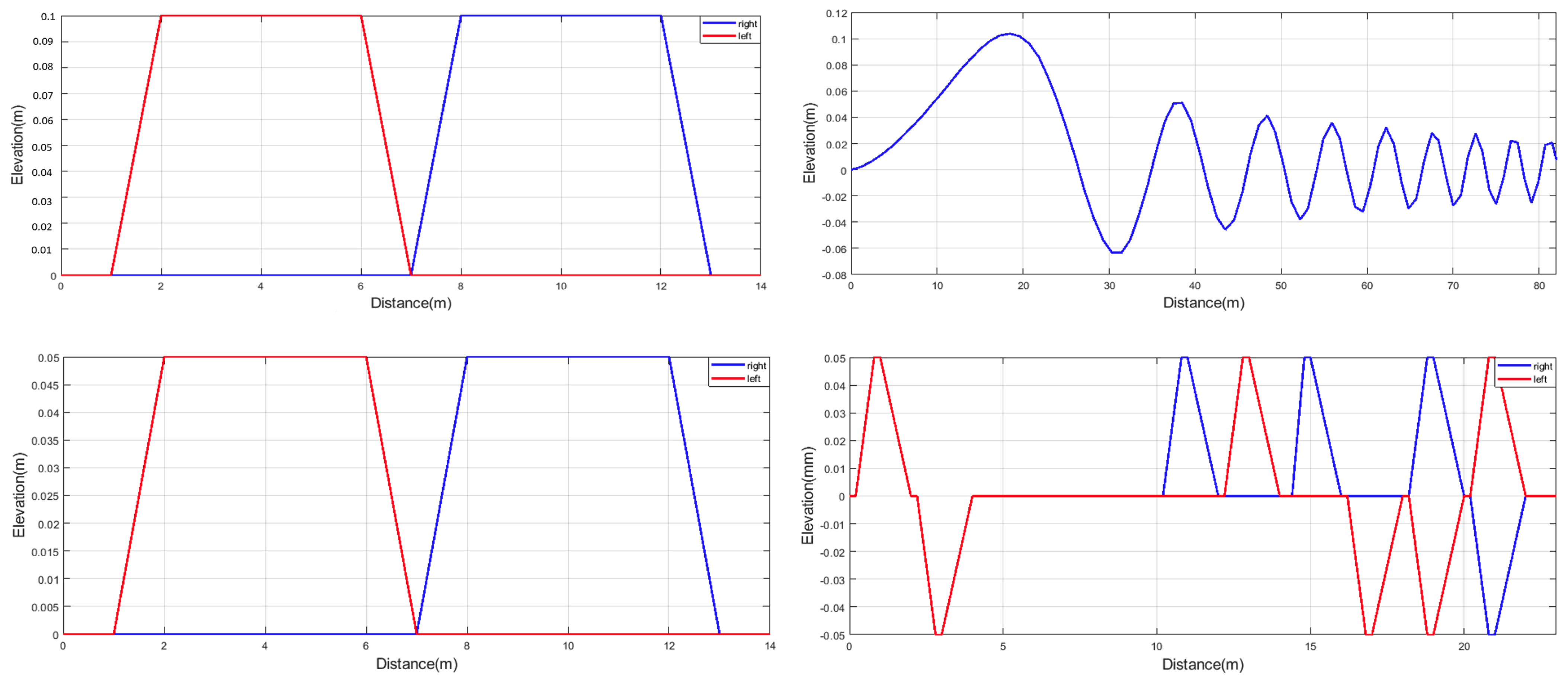
Table 4. The four road irregularities were used in eight locations of the simulation road.
There are two simulations that were performed in order to demonstrate the effectiveness of the proposed method.
  • Simulation 1: Utility truck with semi-active suspension, scheduling variable, and vehicle velocity as constants.
  • Simulation 2: Utility truck with adaptive semi-active suspension, scheduling variable, and velocity varying depending on the road irregularity.
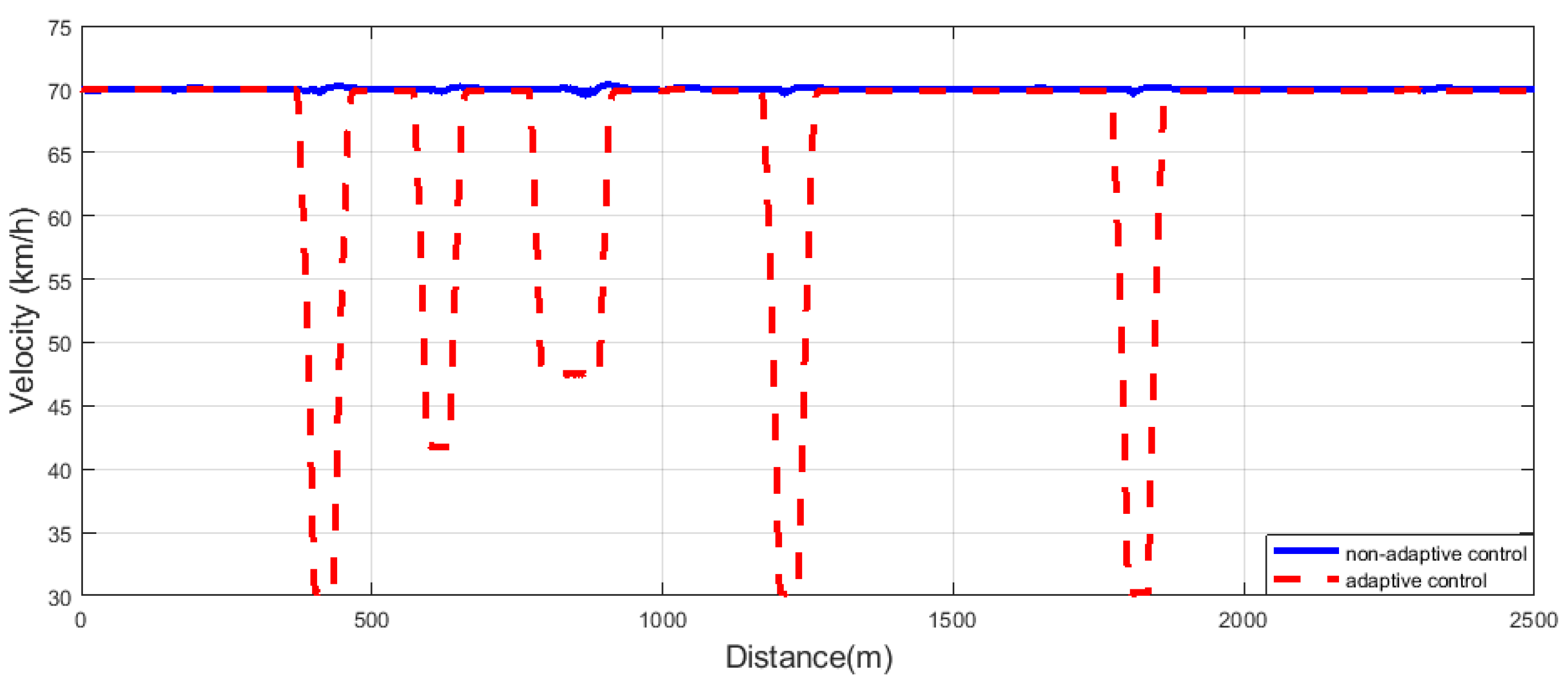
The designed velocity is depicted in 
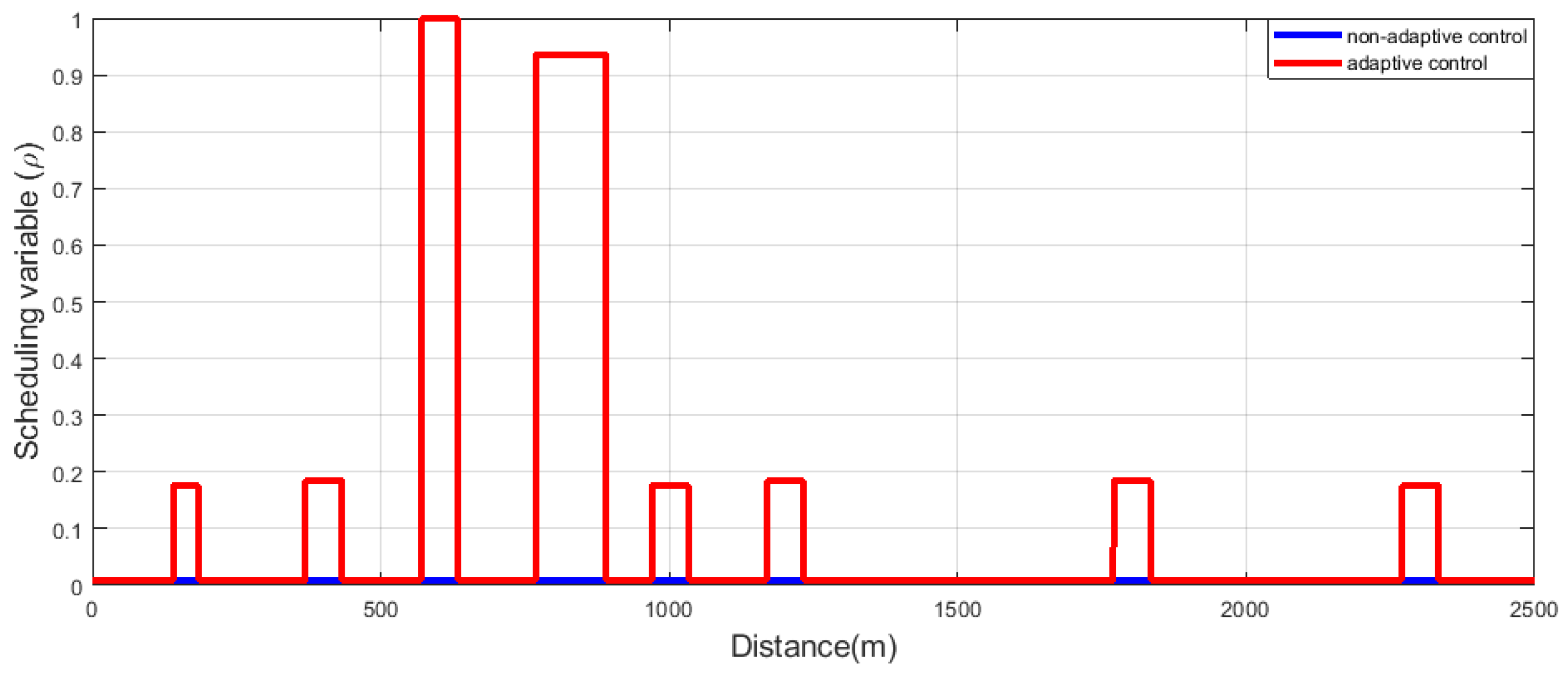
Figure 10, and the designed scheduling variable is shown in Figure 11. The performance results are depicted with their dedicated figures, and the RMS values of improvement on performances are shown in Table 5. Here, the overall value is the average of each corner of the vehicle. The f L is front-left corner, f R is the front-right corner, r L is the rear-left corner, and r R is the rear-right corner of the vehicle.
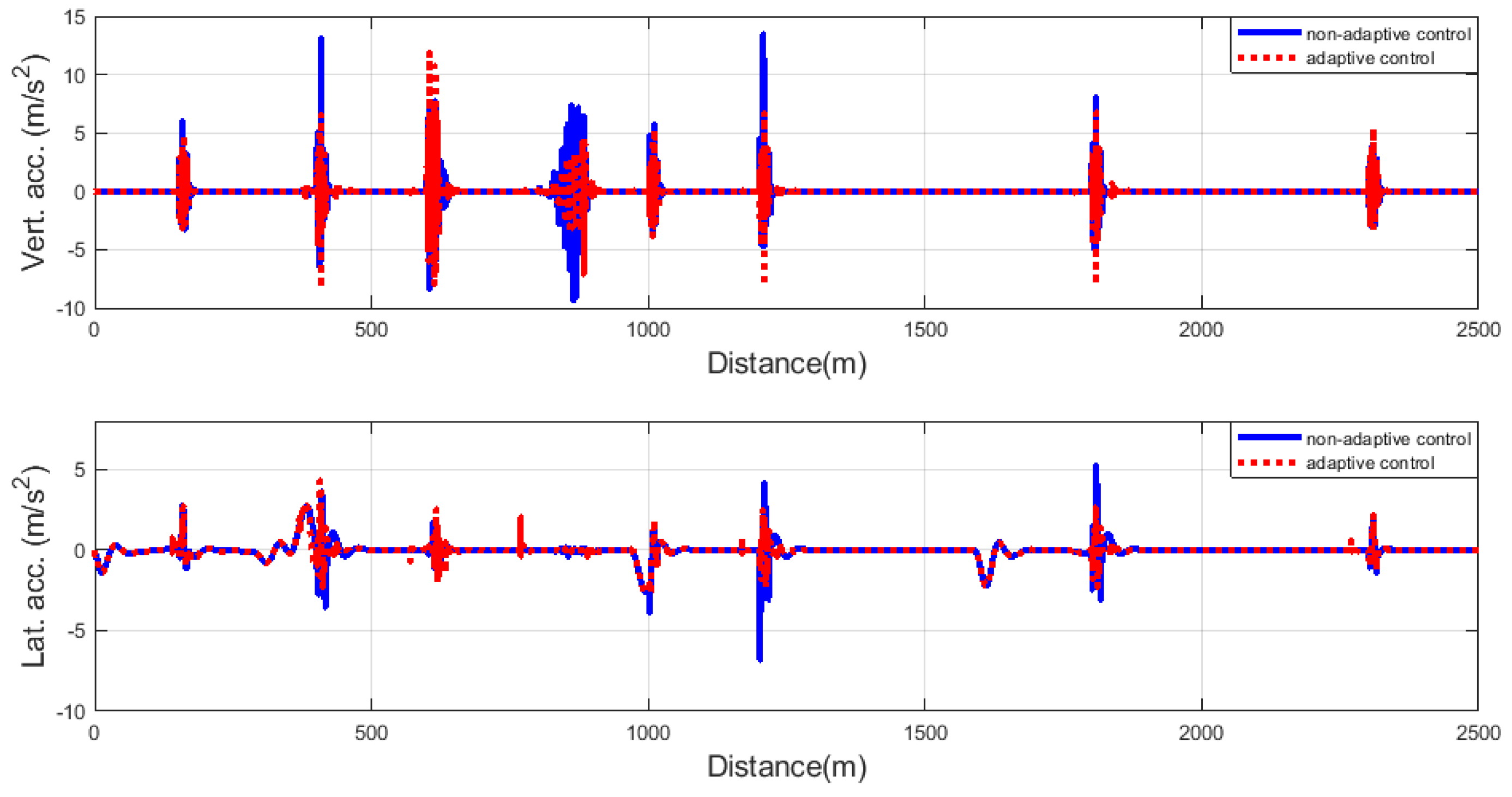
The driving comfort performance is represented by the vertical acceleration of the vehicle. Although lateral acceleration is not a performance in the controller design, it also represents driving comfort. Figure 12 shows both the vertical and lateral acceleration of vehicles in several road irregularities. It is well demonstrated that the accelerations were improved with the proposed adaptivity method. The performance improvement is different for each road irregularity. The greatest improvement was in the second road irregularity, which was 10 cm bumps and located in 400 m, and minor improvement occurred in 5 cm bumps because of their small value. In all irregularities, the adaptive method had smaller acceleration values except the sine-sweep irregularity, and the RMS of accelerations for each irregularity is smaller for the proposed method. The improvements in both vertical and lateral accelerations are also depicted in Table 5.
The second performance consideration is tire deformation, and it shows the contact between the tire and the road surface. For this reason, this is represented as a road-holding performance. The adaptive method decreased the tire deformation value significantly. The front-left tire deformation had a smaller change in the sine-sweep irregularity, and the most significant improvement was in the several-bumps irregularity. This performance improvement is depicted in Figure 13. The significant improvement can be depicted in the r L tire, and overall improvement was around 10%.
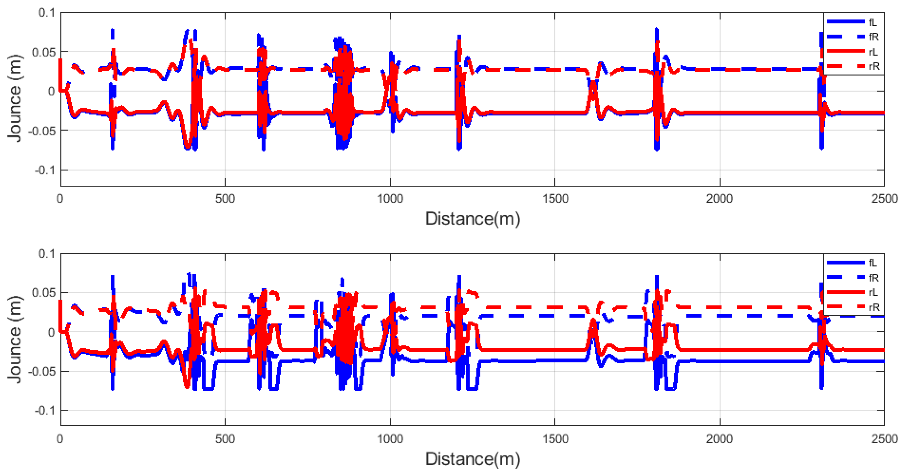
The next performance consideration was vehicle stability, which is presented as a suspension deflection. Vertical deflection between sprung and unsprung masses gives the stability performance of the vehicle. Overall, the suspension deflection performance was improved, though this improvement was not the same for each road irregularity due to the trade-off that is ensured by the scheduling variable. The results of the suspension deflection are shown in Figure 14. The significant improvements were for the sine-sweep road irregularity and several bumps at 600 and 800 m, respectively. Improvements at other locations were not that large due to the improvement in driving comfort performance. The overall improvement in the suspension deflection was negative; it can be said that there was no overall improvement in suspension deflection, whereas the improvement could be observed on f R and r L suspension.
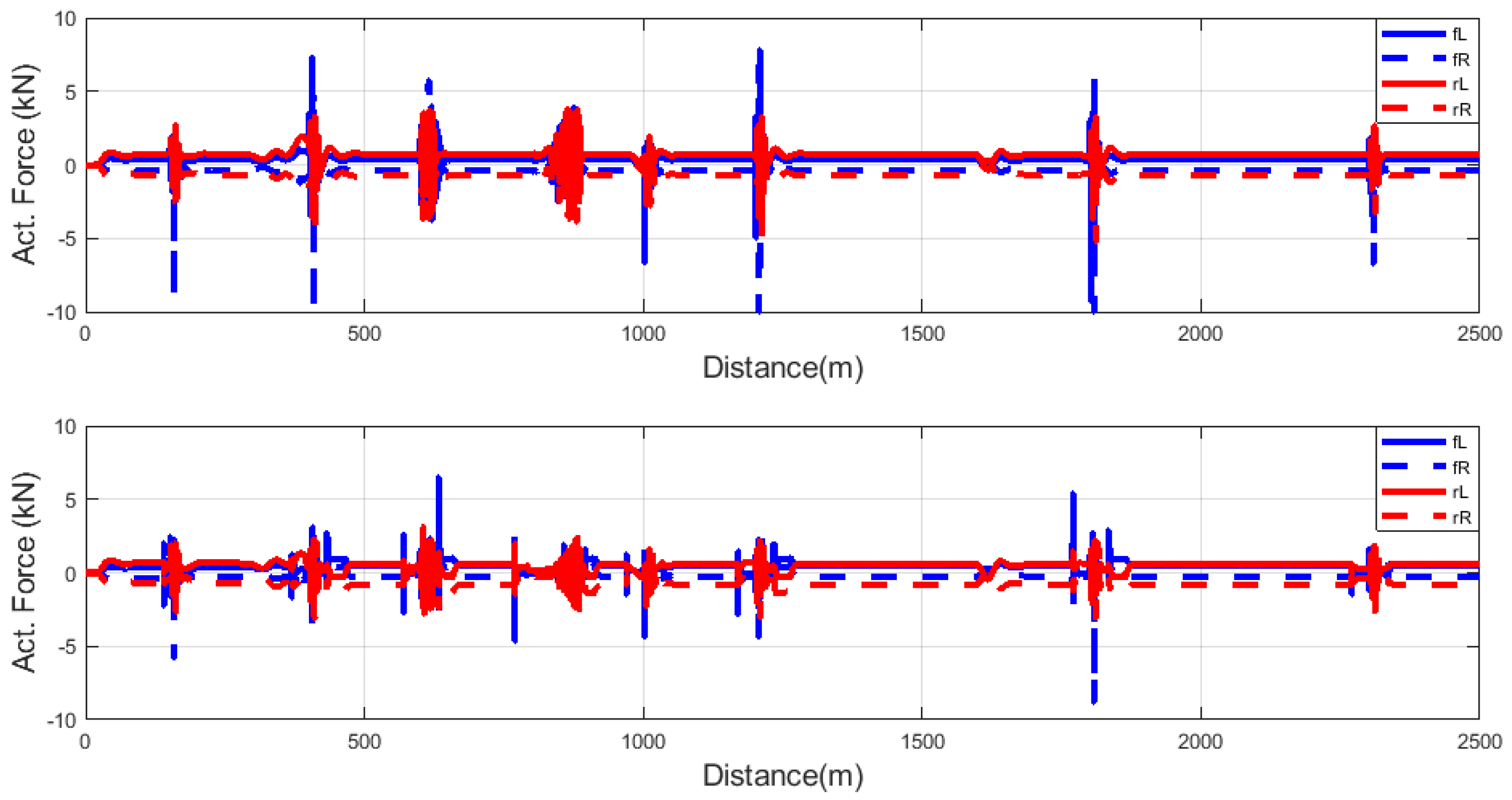
The last performance consideration in the control synthesis is minimizing the control force. For this reason, it is expected that control forces will be reduced with the adaptive method. Despite other performance considerations, the control force weighting function does not contain the scheduling variable; thus, the control forces are minimized with the proposed controller compared to the uncontrolled suspension. The reason why control force is minimized in the adaptive method is an improvement in other performances. This performance is depicted in Figure 15, where we can see the actuated forces were reduced with an adaptive method. It is well shown that the controller forces were decreased for each road irregularity. The biggest reduction was for the 10 cm bumps irregularity. The overall improvement in the control force was nearly 15%, whereas the most significant improvement was the r L damper force with nearly 25%.

6. Discussion

Several research papers were analyzed in order to find a gap in the adaptive semi-active suspension controller, and this detailed literature review showed that a road-adaptive semi-active suspension controller with an integrated cruise controller had not been studied before with a road database. The problem was stated as the current available semi-active suspension systems not being adaptive for different road irregularities or integrating cruise control. The solution to this problem was proposed as designing an online, reconfigurable, road-adaptive, semi-active suspension controller; then, we designed a velocity-focused and velocity-tracking controller. Integration of an adaptive semi-active suspension controller into the integrated cruise control with the road adaptivity method finalizes the solution to the stated problem. The simulation results were analyzed, and these results demonstrated that the adaptive method improved the performances of vehicles with different road irregularities and vehicle velocities.

7. Conclusions

This article introduced the integration of cruise control and an intelligent road-adaptive semi-active suspension control system. The intelligent semi-active suspension controller and velocity-tracking controller were designed through the LPV method, and road adaptation was performed with a road adaptivity algorithm that considers road irregularities and vehicle velocity. The road adaptivity algorithm calculates the dedicated scheduling variable that modifies the behavior of the LPV controller. This behavior of operation mode provides a trade-off between driving comfort and vehicle stability performance. The cruise control part contains a velocity design and tracking controller. The velocity design is based on the ISO 2631-1 standard, the created database, and look-ahead road information. The comfort level must be selected in order to calculate dedicated velocity for road irregularity. The velocity was tracked with a velocity-tracking controller, the designed controllers were integrated, and the operation of the integrated method was validated by real geographical road data that were integrated into a TruckSim simulation environment. In the 2500 m simulation route, eight locations with four different road irregularities were simulated. The results show that the introduced adaptive control method improved vehicles’ performances by ensuring the trade-off between performances.

Author Contributions

Conceptualization, H.B. and A.M.; methodology, H.B.; software, H.B.; validation, H.B.; formal analysis, P.G.; investigation, P.G.; resources, H.B. and A.M.; data curation, H.B.; writing—original draft preparation, H.B.; writing—review and editing, H.B., A.M. and P.G.; visualization, H.B.; supervision, P.G.; project administration, P.G. and O.S.; funding acquisition, P.G. All authors have read and agreed to the published version of the manuscript.

Funding

The research presented in this paper, carried out by the Institute for Computer Science and Control, was supported by the Ministry for Innovation and Technology and the National Research, Development and Innovation Office within the framework of the National Lab for Autonomous Systems. The research was also supported by the National Research, Development and Innovation Office through the project “Cooperative emergency trajectory design for connected autonomous vehicles” (NKFIH: 2019-2.1.12-TÉT_VN).

Data Availability Statement

Not applicable.

Conflicts of Interest

The authors declare no conflict of interest.

References

  1. Soliman, A.; Kaldas, M. Semi-active suspension systems from research to mass-market–A review. J. Low Freq. Noise Vib. Act. Control 2021, 40, 1005–1023. [Google Scholar] [CrossRef]
  2. Savaresi, S.M.; Poussot-Vassal, C.; Spelta, C.; Sename, O.; Dugard, L. Robust “LPV Semi-Active” Control. In Semi-Active Suspension Control Design for Vehicles; Elsevier Ltd.: Amsterdam, The Netherlands, 2010; pp. 139–165. [Google Scholar] [CrossRef]
  3. Pham, T.P. LPV Observer and Fault-Tolerant Control of Vehicle Dynamics: Application to an Automotive Semi-Active Suspension System. Ph.D. Thesis, Université Grenoble Alpes, Saint-Martin-d’Hères, France, 2020. [Google Scholar]
  4. Heißing, B.; Ersoy, M. Chassis Handbook: Fundamentals, Driving Dynamics, Components, Mechatronics, Perspectives; Springer Science & Business Media: Cham, Switzerland, 2010. [Google Scholar]
  5. Gillespie, T. Fundamentals of Vehicle Dynamics; SAE International: Warrendale, PA, USA, 1992. [Google Scholar]
  6. Savaia, G.; Formentin, S.; Panzani, G.; Corno, M.; Savaresi, S.M. Enhancing skyhook for semi-active suspension control via machine learning. IFAC J. Syst. Control. 2021, 17, 100161. [Google Scholar] [CrossRef]
  7. Díaz-Choque, C.S.; Félix-Herrán, L.; Ramírez-Mendoza, R.A. Optimal Skyhook and Groundhook Control for Semiactive Suspension: A Comprehensive Methodology. Shock Vib. 2021, 2021, 8084343. [Google Scholar] [CrossRef]
  8. Mai, V.N.; Yoon, D.S.; Choi, S.B.; Kim, G.W. Explicit model predictive control of semi-active suspension systems with magnetorheological dampers subject to input constraints. J. Intell. Mater. Syst. Struct. 2020, 31, 1157–1170. [Google Scholar] [CrossRef]
  9. Wang, S.Q.; Li, N. Semi-active vibration control for offshore platforms based on LQG method. J. Mar. Sci. Technol. 2021, 21, 9. [Google Scholar]
  10. Morato, M.M.; Normey-Rico, J.E.; Sename, O. Short-sighted robust lpv model predictive control: Application to semi-active suspension systems. In Proceedings of the 2021 European Control Conference (ECC), Delft, The Netherlands, 29 June–2 July 2021; pp. 1525–1530. [Google Scholar]
  11. Yang, L.; Wang, R.; Ding, R.; Liu, W.; Zhu, Z. Investigation on the dynamic performance of a new semi-active hydro-pneumatic inerter-based suspension system with MPC control strategy. Mech. Syst. Signal Process. 2021, 154, 107569. [Google Scholar] [CrossRef]
  12. Sharma, R.C.; Palli, S.; Sharma, N.; Sharma, S.K. Ride Behaviour of a Four-wheel Vehicle using H Infinity Semi-active Suspension Control under Deterministic and Random Inputs. Int. J. Veh. Struct. Syst. (IJVSS) 2021, 13, 234–237. [Google Scholar] [CrossRef]
  13. Ding, R.; Wang, R.; Meng, X.; Chen, L. Research on time-delay-dependent H/H2 optimal control of magnetorheological semi-active suspension with response delay. J. Vib. Control. 2022, 10775463211064380. [Google Scholar] [CrossRef]
  14. Basargan, H.; Mihály, A.; Gáspár, P.; Sename, O. An LPV-Based Online Reconfigurable Adaptive Semi-Active Suspension Control with MR Damper. Energies 2022, 15, 3648. [Google Scholar] [CrossRef]
  15. Basargan, H.; Mihály, A.; Gáspár, P.; Sename, O. Integrated multi-criteria velocity and semi-active suspension control based on look-ahead road information. In Proceedings of the 2020 28th Mediterranean Conference on Control and Automation (MED), Saint-Raphaël, France, 15–18 September 2020; pp. 25–30. [Google Scholar]
  16. Hu, H.; Wu, G.; Mao, L. Preview Control of Semi-Active Suspension with Adjustable Damping Based on Machine Vision. In Proceedings of the 2021 IEEE 16th Conference on Industrial Electronics and Applications (ICIEA), Chengdu, China, 1–4 August 2021; pp. 117–123. [Google Scholar] [CrossRef]
  17. Li, Z.; Kolmanovsky, I.; Atkins, E.; Lu, J.; Filev, D.; Michelini, J. Cloud aided semi-active suspension control. In Proceedings of the 2014 IEEE Symposium on Computational Intelligence in Vehicles and Transportation Systems (CIVTS), Orlando, FL, USA, 9–12 December 2014; pp. 76–83. [Google Scholar] [CrossRef]
  18. Theunissen, J.; Tota, A.; Gruber, P.; Dhaens, M.; Sorniotti, A. Preview-based techniques for vehicle suspension control: A state-of-the-art review. Annu. Rev. Control 2021, 51, 206–235. [Google Scholar] [CrossRef]
  19. Tran, G.Q.B.; Pham, T.P.; Sename, O.; Costa, E.; Gaspar, P. Integrated Comfort-Adaptive Cruise and Semi-Active Suspension Control for an Autonomous Vehicle: An LPV Approach. Electronics 2021, 10, 813. [Google Scholar] [CrossRef]
  20. Basargan, H.; Mihály, A.; Gáspár, P.; Sename, O. Integrated adaptive velocity and semi-active suspension control for different road profiles. In Proceedings of the 2022 30th Mediterranean Conference on Control and Automation (MED), Vouliagmeni, Greece, 28 June–1 July 2022; pp. 933–938. [Google Scholar]
  21. Bokor, J.; Balas, G. Linear Parameter Varying Systems: A Geometric Theory and Applications. In Proceedings of the 16th IFAC World Congress, Prague, Czech Republic, 3–8 July 2005. [Google Scholar]
  22. Wu, F.; Yang, X.H.; Packard, A.; Becker, G. Induced l2-norm control for LPV systems with bounded parameter variation rates. Int. J. Nonlinear Robust Control 1996, 6, 983–998. [Google Scholar] [CrossRef]
  23. Yu, J.; Sideris, A. Hinf control with parametric Lyapunov functions. Syst. Control Lett. 1997, 30, 57–69. [Google Scholar] [CrossRef]
  24. Zuo, L.; Nayfeh, S. Low order continuous-time filters for approximation of the ISO 2631-1 human vibration sensitivity weightings. J. Sound Vib. 2003, 265, 459–465. [Google Scholar] [CrossRef]
  25. 2631-1; Mechanical Vibration and Shock-Evaluation of Human Exposure to Whole-Body Vibration-Part 1: General Requirements. ISO: Geneva, Switzerland, 1997.
  26. Xiong, Y.; Yang, X. A review on in-tire sensor systems for tire-road interaction studies. Sens. Rev. 2018, 38, 231–238. [Google Scholar] [CrossRef]
  27. Xiong, Y.; Tuononen, A. A laser-based sensor system for tire tread deformation measurement. Meas. Sci. Technol. 2014, 25, 115103. [Google Scholar] [CrossRef]
  28. Heidarian, A.; Wang, X. Review on Seat Suspension System Technology Development. Appl. Sci. 2019, 9, 2834. [Google Scholar] [CrossRef] [Green Version]
Figure 1. Force-piston velocity diagram of different kinds of ideal dampers.
Machines 11 00204 g001
Figure 3. Closed-loop interconnection structure of semi-active suspension control.
Machines 11 00204 g003
Figure 5. FWVM values of road profiles at different velocities.
Machines 11 00204 g005
Figure 6. Closed-loop interconnection structure of velocity tracking.
Machines 11 00204 g006
Figure 7. Data collection.
Machines 11 00204 g007
Figure 8. System architecture.
Machines 11 00204 g008
Figure 9. Simulation route.
Machines 11 00204 g009
Figure 10. Velocity profile of the vehicle.
Machines 11 00204 g010
Figure 11. Designed scheduled variable.
Machines 11 00204 g011
Figure 12. Vertical and lateral accelerations.
Machines 11 00204 g012
Figure 13. Tire deformation: non-adaptive (top) and adaptive (bottom).
Machines 11 00204 g013
Figure 14. Suspension deflection: non-adaptive (top) and adaptive (bottom).
Machines 11 00204 g014
Figure 15. Control forces: non-adaptive (top) and adaptive (bottom).
Machines 11 00204 g015
Table 1. Suspension parameters.
Parameters
(Symbols)
Front
Suspension
Rear
Suspension
Unit
sprung mass ( m s )214336kg
unsprung mass ( m u )4040kg
suspension stiffness ( k s )3060kN/m
tire stiffness ( k t )220220kN/m
damping ( b s )5050N/m/s
time constant ( τ )0.010.01s
Table 2. Data stored in the database.
Velocity (km/h)Vertical Acceleration (RMS)
Road IRoad IIRoad IIIRoad IV
10 0.04650.30060.43250.1496
200.27360.96631.03170.3275
300.96171.56781.24840.491
401.28092.55081.50970.7937
501.7012.10062.00020.8654
601.90612.5732.65121.0931
702.90313.22813.07211.1052
802.90823.59513.80781.8764
902.90185.34094.19931.4656
1002.94485.62334.30452.0262
1103.62546.20468.56762.3574
Table 3. ISO 2631-1:1997, magnitudes of overall vibration [25].
Frequency-Weighted Vibration Magnitude (FWVM)Likely Reaction in Public Transport
Less than 0.315 m/s 2 Not uncomfortable
0.315–0.63 m/s 2 A little uncomfortable
0.5–1 m/s 2 Fairly uncomfortable
0.8–1.6 m/s 2 Uncomfortable
1.25–2.5 m/s 2 Very uncomfortable
Greater than 2 m/s 2 Extremely uncomfortable
Table 4. Road profile data.
Road ProfileLocation [m]Velocity [km/h] ρ
1Road IV150700.1758
2Road II40030.330.1838
3Road III60041.840.99
4Road I80047.60.9367
5Road IV1000700.1758
6Road II120030.330.1838
7Road II180030.330.1838
8Road IV2300700.1758
Table 5. Performance improvement with an adaptive method.
PerformanceNon-AdaptiveAdaptive
Vertical Acceleration0.84760.8307
Lateral Acceleration0.52300.4855
Suspension DeflectionfL0.03010.0309
fR0.02930.0242
rL0.02730.0224
rR0.02730.0298
Overall0.02580.0268
Tire DeformationfL0.00650.0061
fR0.00490.0043
rL0.00600.0046
rR0.00590.0057
Overall0.00580.0052
Control ForcefL516.81498.36
fR529.57344.50
rL811.35608.90
rR811.64813.00
Overall667.34566.19
Disclaimer/Publisher’s Note: The statements, opinions and data contained in all publications are solely those of the individual author(s) and contributor(s) and not of MDPI and/or the editor(s). MDPI and/or the editor(s) disclaim responsibility for any injury to people or property resulting from any ideas, methods, instructions or products referred to in the content.

