Article

A Rolling Bearing Fault Diagnosis Method Based on Switchable Normalization and a Deep Convolutional Neural Network

1
College of Intelligent Systems Science and Engineering, Harbin Engineering University, Harbin 150001, China
2
College of Power and Energy Engineering, Harbin Engineering University, Harbin 150001, China
*
Author to whom correspondence should be addressed.
Machines 2023, 11(2), 185; https://doi.org/10.3390/machines11020185
Submission received: 12 December 2022 / Revised: 16 January 2023 / Accepted: 26 January 2023 / Published: 30 January 2023
(This article belongs to the Section Machines Testing and Maintenance)

Abstract

:
Aiming to address the problems of a low fault detection rate and poor diagnosis performance under different loads and noise environments, a rolling bearing fault diagnosis method based on switchable normalization and a deep convolutional neural network (SNDCNN) is proposed. The method effectively extracted the fault features from the raw vibration signal and suppressed high-frequency noise by increasing the convolution kernel width of the first layer and stacking multiple layers’ convolution kernels. To avoid losing the intensity information of the features, the K-max pooling operation was adopted at the pooling layer. To solve the overfitting problem and improve the generalization ability, a switchable normalization approach was used after each convolutional layer. The proposed SNDCNN was evaluated with two sets of rolling bearing datasets and obtained a higher fault detection rate than SVM and BP, reaching a fault detection rate of over 90% under different loads and demonstrating a better anti-noise performance.

1. Introduction

Rolling bearings are one of the main components of mechanical equipment. The online monitoring of the real-time operation of bearings and the accurate identification of fault types and fault degrees can ensure the reliability of mechanical equipment operation [1,2]. One of the most widely used methods to detect rolling bearing faults by vibration signals is to extract the characteristics of the vibration signals through techniques such as time-domain analysis [3], wavelet analysis, wavelet packet analysis [4,5,6], empirical wavelet transform [7,8], empirical mode decomposition [9], ensemble empirical mode decomposition [5,10], sparse decomposition [11], independent component analysis [12], and spectral kurtosis [13,14]. However, the characteristics of bearing faults under different operating conditions and noise environments are complex, and effectively mining information from bearing vibration data has always been an important problem in rolling bearing fault diagnosis [15,16,17].
Fault diagnosis is essentially pattern recognition. The currently commonly used approaches of support vector machines (SVMs) [18,19,20], random forests [21], AdaBoost [22], backpropagation neural networks [23], and radial basis neural networks [24] are shallow learning models with a limited fault feature expression ability, and the accuracy of the diagnosis is subject to the feature extraction results. In recent years, researchers have turned their attention to various deep learning models, such as convolutional neural networks (CNNs) [25], recurrent neural networks [26], autoencoders [27,28,29], and transfer learning [30]. Among these, CNNs can convert the original features of the input layer by layer into features that are easy to recognize and realize the deep characterization of rolling bearing faults, representing a hotspot of current research [31,32]. Several studies have applied CNNs as a classifier, using wavelet packets [33,34,35], continued wavelet transform [36,37], dual-tree complex wavelet transform [38,39], fast Fourier transform (FFT) [40], discrete wavelet transform (DWT) [40], and other signal processing methods [41] to pre-process one-dimensional vibration signals, which are converted into the time domain or the time-frequency domain and then input into the CNN for fault diagnosis [42]. This processing method fails to fully exploit CNNs’ deep learning ability. Therefore, dislocated time series (DTS) [43]; gray-scale images [44,45], infrared thermal images, and other image data [46,47]; one-dimensional CNNs [48,49]; and other methods have been proposed to reshape the input data dimension and get rid of the dependence on expert knowledge for vibration signal feature extraction. However, in most current studies, the pooling operation of CNNs mostly adopts the max-pooling method. Since the rolling bearing is a periodic time-series signal, this processing method causes the intensity information of the feature to be lost. In response to this shortcoming, the deep convolutional neural network (DCNN) model presented in this paper used the K-max pooling method, which could retain the Top-K score of all feature values, thereby avoiding the problem of the loss of intensity information in the signal.
Furthermore, although feature extraction can be effectively performed through the superposition of multiple convolutional layers and pooling layers, it is easy to cause overfitting. Therefore, in this study we adopted the switchable normalization (SN) method [50], which could choose the appropriate normalization method for each normalization layer of the DCNN. Experiments showed that the average recognition rate of the proposed SNDCNN model was 99.68%, and it achieved good diagnostic results under different loads and noise environments.
The remainder of this paper is structured as follows. The next section presents an interpretation of the relevant literature, including works on CNN and K-max pooling. In Section 3, we propose a novel model combining SN and DCNN. Then, in Section 4, we describe in detail the experimental procedures and diagnosis result analysis based on two rolling bearing datasets. Finally, the conclusions are presented in Section 5.

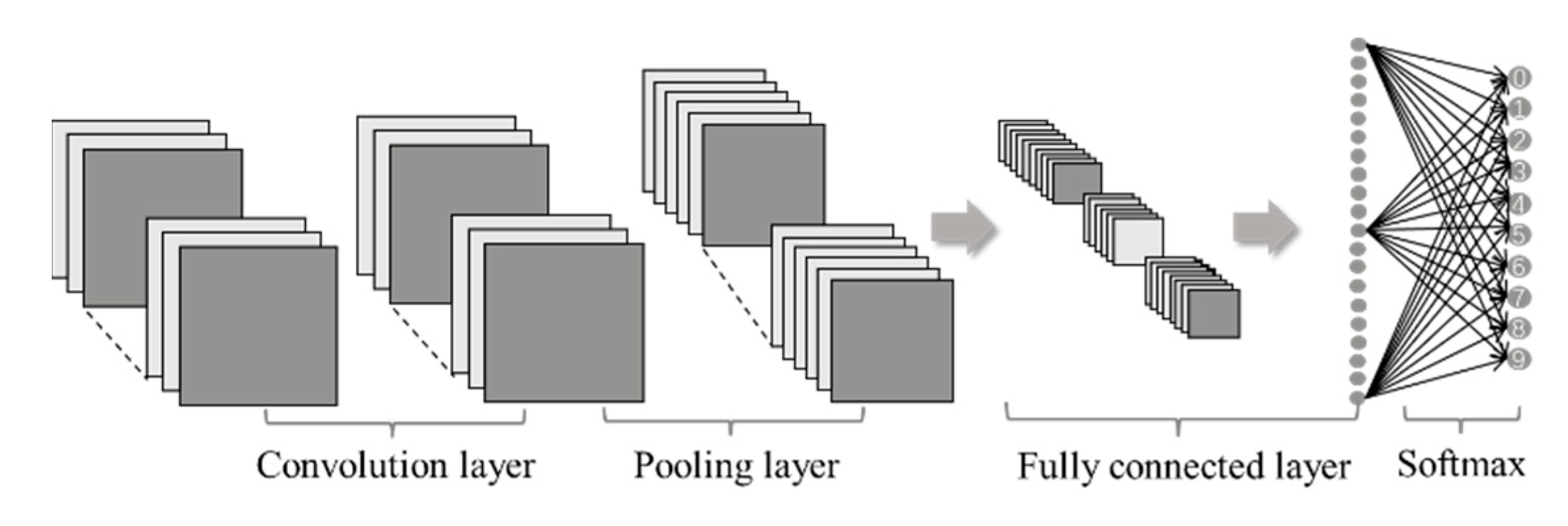
2. Convolutional Neural Network

The main CNN hierarchy is shown in Figure 1.

2.1. Convolution Layer
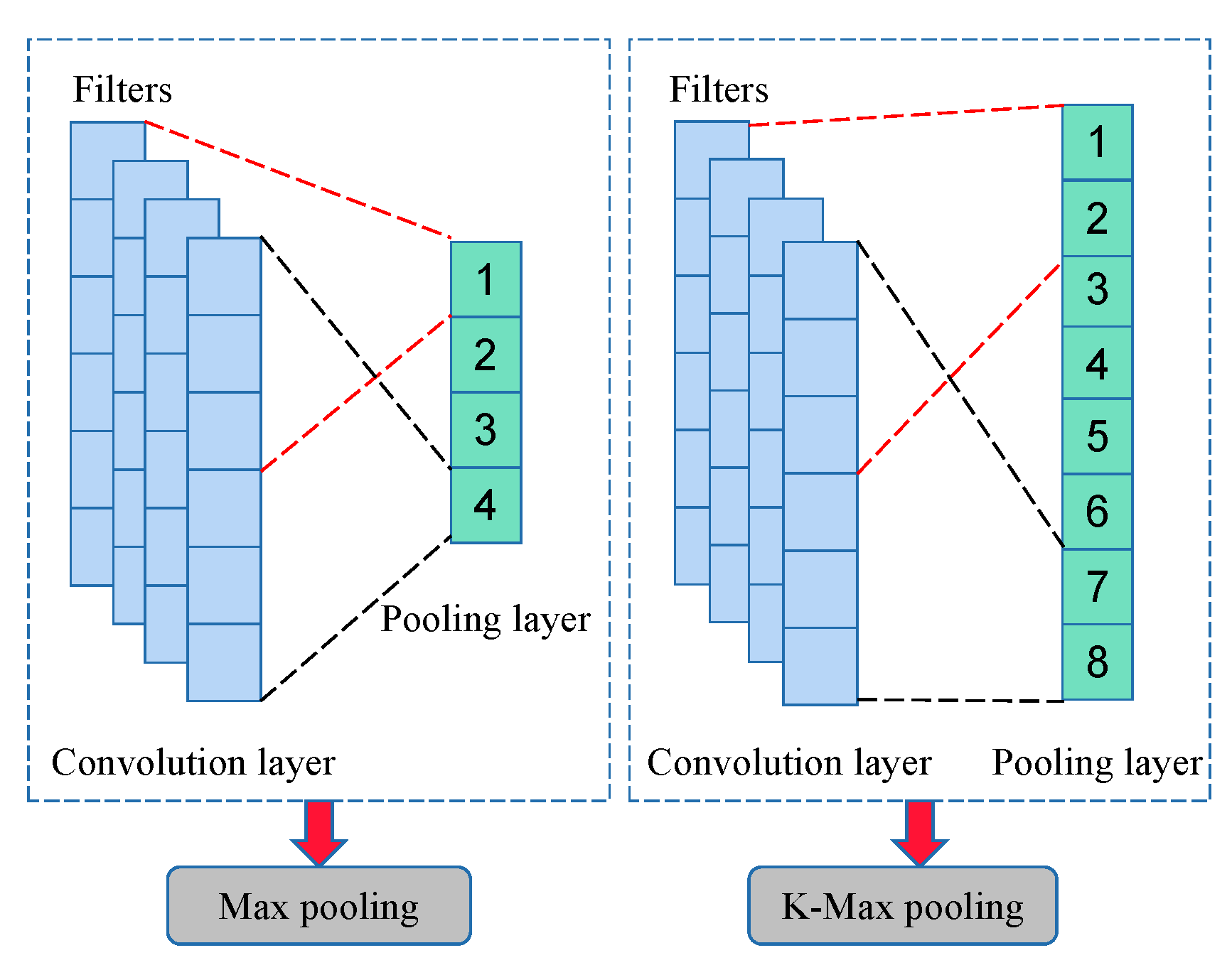
In the convolution layer, the convolution calculation is performed on the input through the convolution kernel, and each small block in the neural network is analyzed more deeply to obtain higher abstraction features.
X j k = f i M j X i k 1 W i j k + b j k
where Xjk is the jth element of the kth layer; Mj is the input feature vector; Xik−1 is the element; Wijk is the weight matrix of the convolution kernel; bjk is the bias term; and ƒ(·) is the activation function, which is a non-linear function that converts the output of each neuron from linear to non-linear. In this model, the Relu function is chosen as the activation function.
f x = max x , 0

2.2. Pooling Layer

After the feature extraction of the input data through the convolution layer, the resulting data dimension is still relatively large. The pooling layer does not change the depth of the data matrix of the previous layer. By reducing the size of the data matrix, the goal of reducing the parameters in the neural network is achieved. The mathematical expression of the pooling layer is shown in Equation (3):
X = f α d o w n x + b
where x is the output, ƒ(·) is the activation function, α is the multiplicative bias, down( ) is the downsampling function, and b is the bias term.
Commonly used pooling layer processing methods include general pooling, overlapping pooling, average pooling, and max pooling. In this study, K-max pooling was selected, which is an improved maximum pooling method. A comparison chart for max pooling and K-max pooling when K = 2 is shown in Figure 2. The max pooling method has an obvious disadvantage in that sometimes certain strong features appear multiple times. The more occurrences, the stronger the feature. Because maximum pooling only retains a maximum value, which means that the same feature has incomplete intensity information, K-max pooling can retain all feature values scored in Top-K and the original order of these feature values, thus providing more complete feature information for subsequent use.

2.3. Fully Connected Layer

The fully connected layer acts as a classifier in the CNN. It accepts the input of the previous neural layer and outputs an N-dimensional vector, where N is the total number of all possible categories. After the processing of multiple convolutional layers and pooling layers, the final classification results are generally provided by one or two fully connected layers. This study used the Softmax layer for classification.

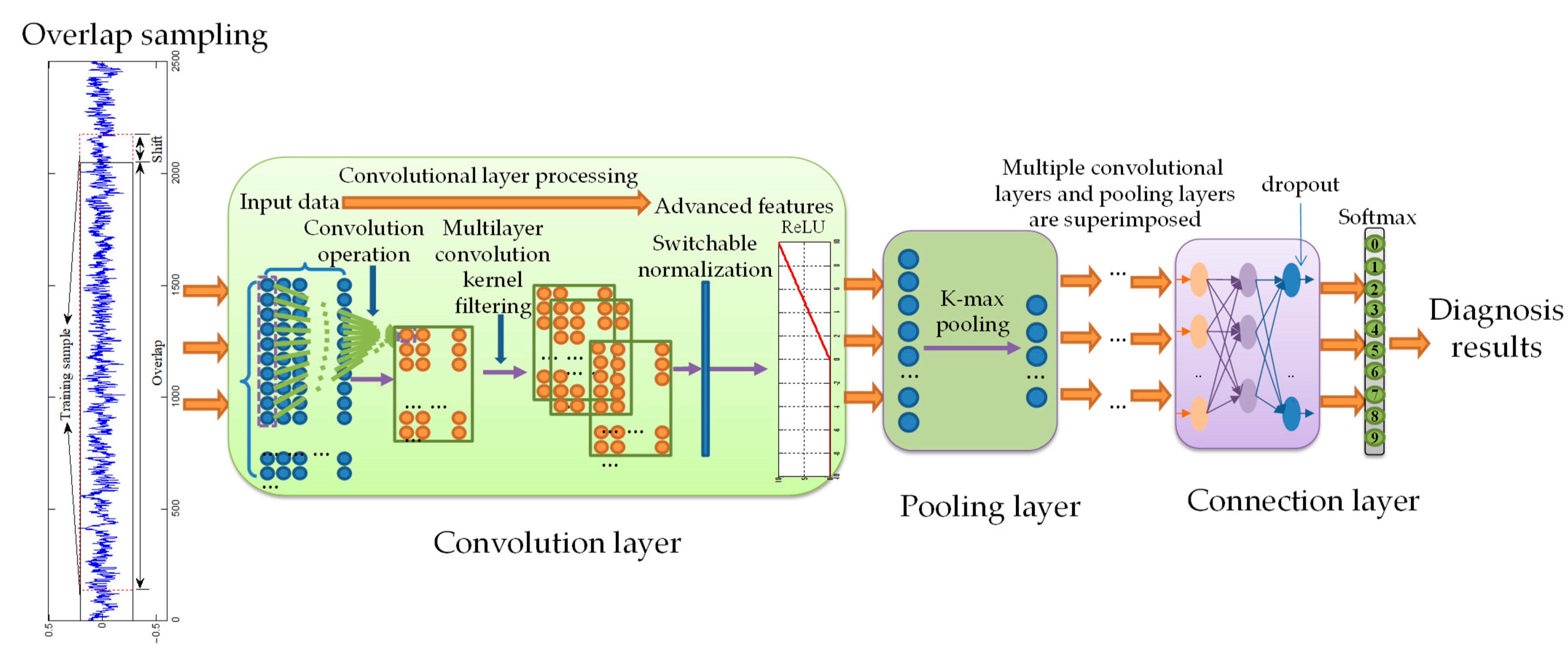
3. Rolling Bearing Fault Diagnosis Method Based on SNDCNN

Although traditional CNNs have a high recognition rate for the fault diagnosis of rolling bearings, the recognition rate still needs to be improved, as it cannot meet the challenge of bearing fault diagnosis under different loads and noise environments. In response to these problems, a new rolling bearing fault diagnosis method based on switchable normalization and a deep convolutional network (SNDCNN) was proposed, as shown in Figure 3.

3.1. Structural Parameters of the SNDCNN

In this study, by increasing the convolution kernel width of the DCNN’s first layer and setting the convolution kernel size of the first layer to 80 × 1, a larger receptive field could be obtained, which could effectively extract one-dimensional vibration signal characteristics and suppress high-frequency noise. The subsequent neural layers adopted a multi-layer convolution kernel stacking to achieve multi-layer nonlinear mapping. However, increasing the width of the convolution kernel and superimposing the convolution layer increases the complexity of the DCNN model and the training parameters, which may cause overfitting problems. To suppress overfitting and increase the training speed, the switchable normalization method was adopted, and the SN process was performed between each convolutional layer and the active layer of the DCNN. The structural parameters of the SNDCNN are shown in Table 1.

3.2. Switchable Normalization

Normalization technology plays an important role in the deep learning model, as it can effectively suppress overfitting and improve the generalization ability of the DCNN. Commonly used normalization methods include batch normalization (BN), instance normalization (IN), layer normalization (LN), and group normalization (GN). However, each normalization method has its limitations in terms of the scenarios to which it can be applied. Although normalization can improve DCNN performance, solving different problems often requires different normalization methods. A DCNN often contains several or even dozens of normalization layers. Selecting the appropriate normalization operation for each normalization layer using a manual takes a lot of time. Thus, the same normalization method is used in traditional deep neural networks.
In this study, the switchable normalization method was proposed to solve the above problems. SN contains three normalization methods: IN, LN, and BN. Using differential learning, the appropriate normalization method for different normalization layers in the deep neural network can be automatically selected. Suppose that the input data of the convolutional layer of a DCNN can be expressed in four dimensions, with each dimension representing the number of samples N, the number of channels C, the height of the channel H, and the width of channel W. Each pixel that is normalized based on the SN method is represented as hncij:
h ^ n c i j = γ h n c i k k Ω ω k μ k k Ω ω k σ k 2 + θ + β
where h ^ n c i j is the normalized pixel value, and n, c, i, and j are the subscripts of the four dimensions. The above definition in Equation (5) is similar to those of BN, IN, and LN. They all learn the scaling factor γ and the offset factor β. The main difference is the statistical information included in SN (mean μ and variance σ2), making it unlike IN, which is only calculated in one channel, and LN, which is only calculated in one layer. In SN, a set is defined as Ω = IN, LN, BN, and the set weighted average is chosen by a suitable approach. ωk and ωk′ are the weight coefficients for the corresponding statistics. The weighting coefficient ωk of the mean is calculated as follows:
ω k = e λ k k I N , L N , B N e λ k , k I N , L N , B N
The calculation methods of the mean and variance of IN, LN, and BN are as follows:
μ I N = 1 H W i , j H , W h n c i j , σ I N 2 = 1 H W i , j H , W h n c i j μ I N 2
μ L N = 1 C c = 1 C μ I N , σ L N 2 = 1 C c = 1 C σ I N 2 + μ I N 2 μ L N 2
μ B N = 1 C n = 1 N μ I N , σ B N 2 = 1 N n = 1 N σ I N 2 + μ I N 2 μ B N 2

3.3. Adaptive Momentum Algorithm

To speed up the convergence speed and accuracy, the adaptive momentum (Adam) algorithm was used to update the parameters and optimize the model. Adam is by far the best-performing gradient descent model optimization algorithm. It can be seen as a combination of the momentum algorithm and the RMSProp algorithm. When updating parameters, Adam considers not only the gradient of the current iteration but also the gradient of all previous iterations and the square of the gradient. By accumulating the gradient index weights, Adam introduces the first- and second-order moment estimates of the parameters into the update operation. Thus, the adaptive change in the learning rate can be realized. The specific steps of the Adam parameter update are as follows:
Steps of Adam parameter update:
Set the learning rate α, the first-order moment estimate exponential decay rate ρ1, the second-order moment estimate exponential decay rate ρ2, and the minimum constant ε. The parameters in this paper are all default values, α = 0.001, ρ1 = 0.9 = 0.9, ρ2 = 0.999, ε = 1 × 10⁻⁸.
Require: Initialize the first-order moment estimate s0 and second-order moment estimate r0 to 0, and initialize the iteration step number t to 0.
Require: Calculate the gradient of the loss function ƒ(θ) for the parameter θ, and loop the following updates:
While θ is not converged do:
1. Update steps: t t + 1
2. Computing the gradients:   g t θ f θ
3. Update biased first moment estimates:   s t ρ 1 s t 1 + 1 ρ 1 g t
4. Update biased second-order moment estimates:   r t ρ 2 r t 1 + 1 ρ 2 g t 2
5. Correct the deviation of the first moment:   s ^ t s t 1 ρ 1 t
6. Correct the deviation of the second moment:   r ^ t r t 1 ρ 2 t
7. Calculation update:   Δ θ α s ^ t r ^ t + ε
8. App update:   θ = θ + Δ θ
End while
Return θ

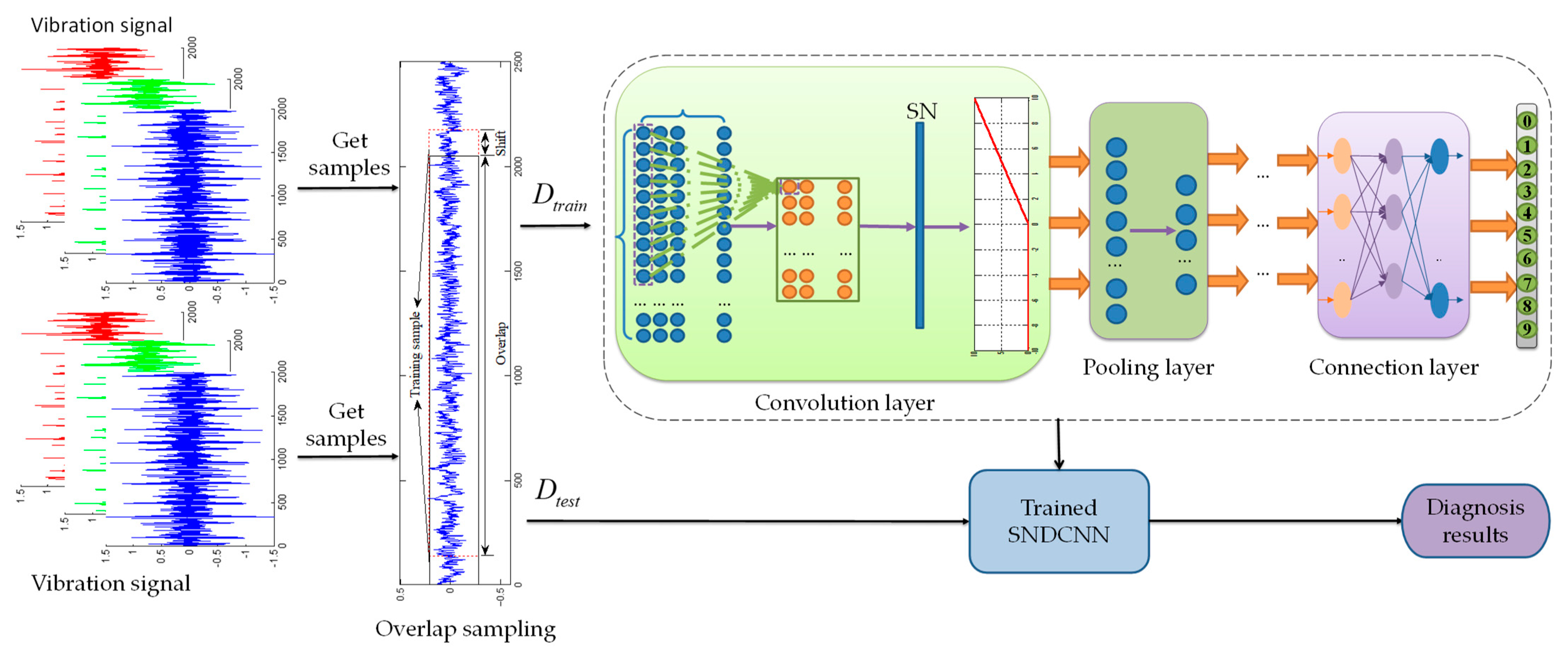
3.4. Fault Diagnostic Process

The algorithm consisted of the following two stages, as shown in Figure 4. The detailed fault diagnosis process flow is as follows:
(1)
Training Stage:
Step 1—data preprocessing: The vibration signals of the rolling bearings were collected, and the original data were expanded by overlapping sampling; then, these were divided into samples of length N, and the training data were input into the SNDCNN.
Step 2—training network: After the training data were input into the first layer of wide convolution kernels, they underwent a non-linear transformation of the ReLU function to become a set of feature maps, which were then put through pooling layer 1 for further feature extraction. The processed data were then input into a continuous six-layer superimposed small convolution kernel layer, which could effectively extract data features. Between each convolutional layer and the activation layer above, a switchable normalization method was used for processing. Together, the dropout rate was 0.5. After the nonlinear transformation of the ReLU function, its output was to the final Softmax layer.
Step 3—well-trained SNDCNN: A well-trained SNDCNN was saved for rolling bearing fault diagnosis.
(2)
Testing Stage:
Step 1—testing data acquisition: New vibration signals were acquired, and segmented samples were obtained as the testing dataset Dtest.
Step 2—testing: Dtest was input into the trained SNDCNN obtained from the training stage, providing the corresponding diagnosis result.

4. Experimental Verification

4.1. Case 1—Western Reserve University Rolling Bearing Data Analysis

The experimental verification in this study was carried out based on the rolling bearing fault dataset of Case Western Reserve University (CWRU). The test rig is shown in Figure 5. The rolling bearing mode was SKF 6205, which contained three fault locations, on the ball, inner ring, and outer ring of the bearing. The diameters of the bearing faults were 0.007 inches, 0.014 inches, and 0.021 inches, respectively.

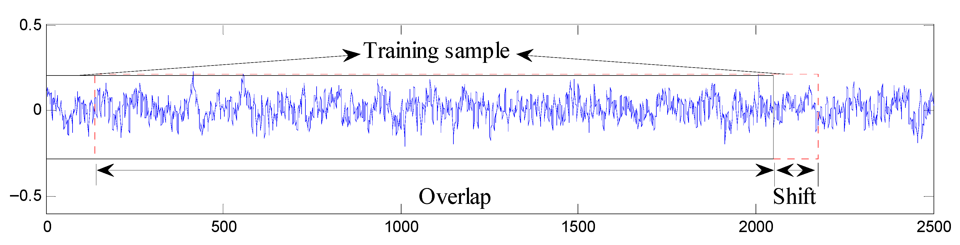
4.1.1. Dataset Division

During the experiment, to avoid the SNDCNN overfitting problem caused by the insufficient amount of data in the training set, the data were expanded by overlapping sampling, that is, starting from the initial sampling point, the data length of each sampling was N. The position of the next sampling was shifted by n from the previous sampling position. The overlapping sampling process is shown in Figure 6:
The dataset division is shown in Table 2. According to the load, the rolling bearing data of Western Reserve University were divided into three situations, A, B, and C, and the corresponding loads were 1 hp, 2 hp, and 3 hp, respectively. Dataset D was the sum of datasets A, B, and C, that is, it contained three different loads at the same time. Take dataset A as an example: it included 10 types of labels, 0–9; each label included 800 training samples, 40 test samples, and 20 verification samples; and each sample had a length of 2048. Dataset D contained 24,000 training samples, 1200 test samples, and 600 verification samples.

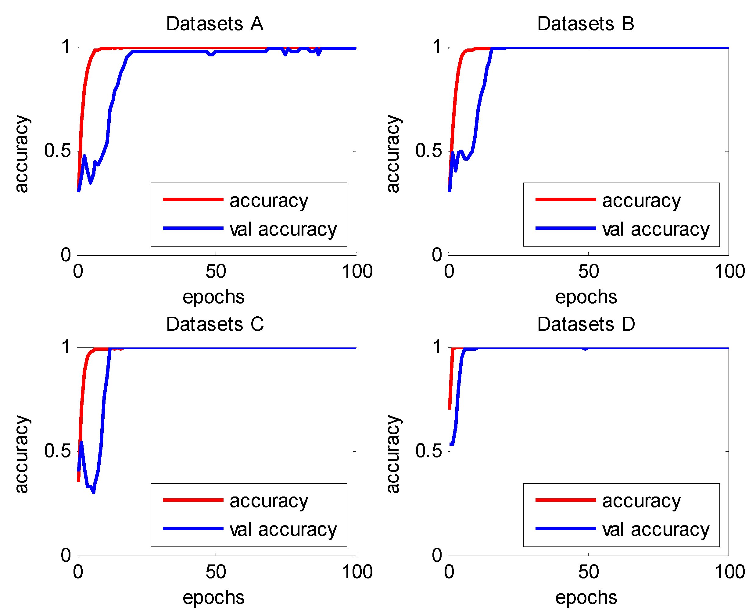
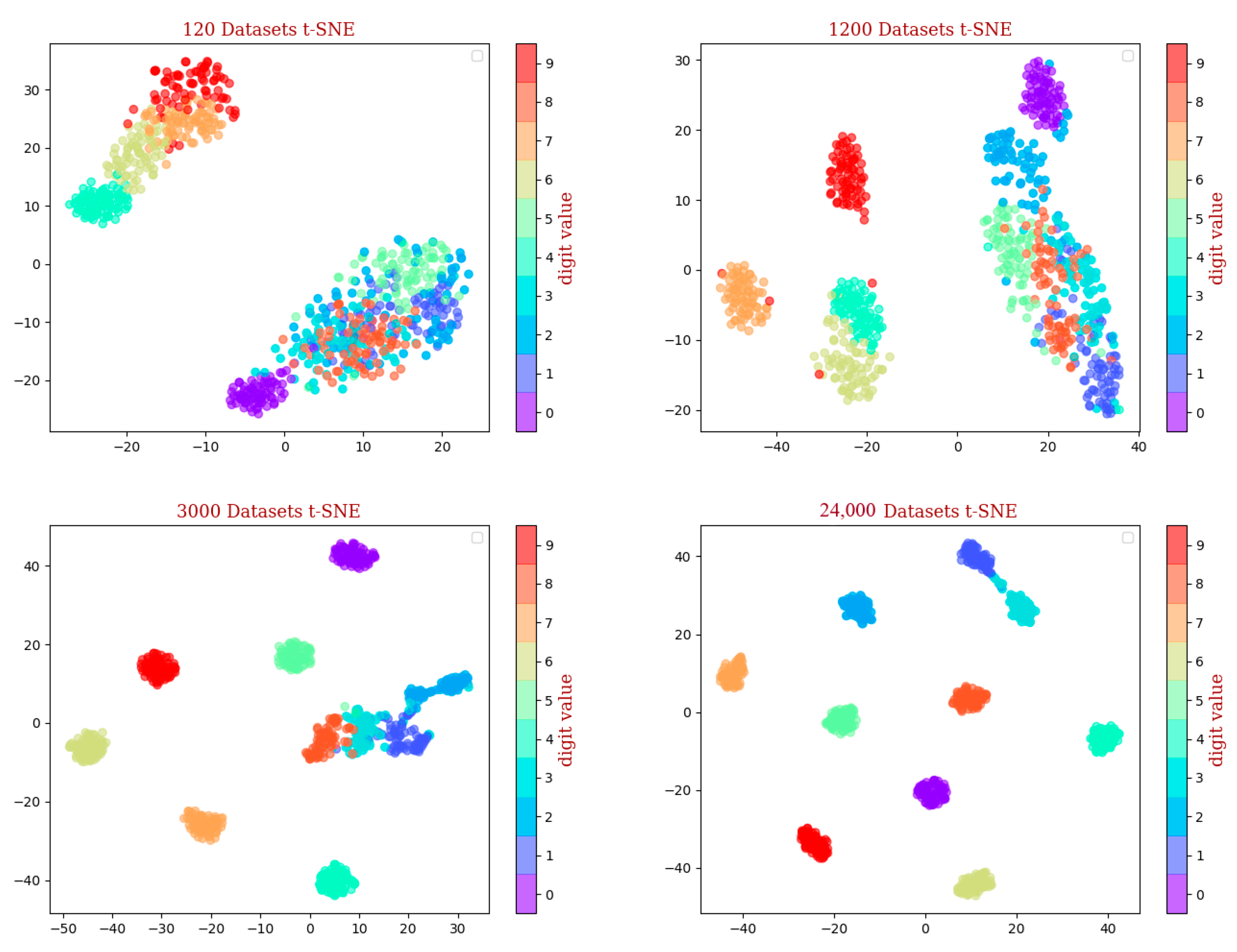
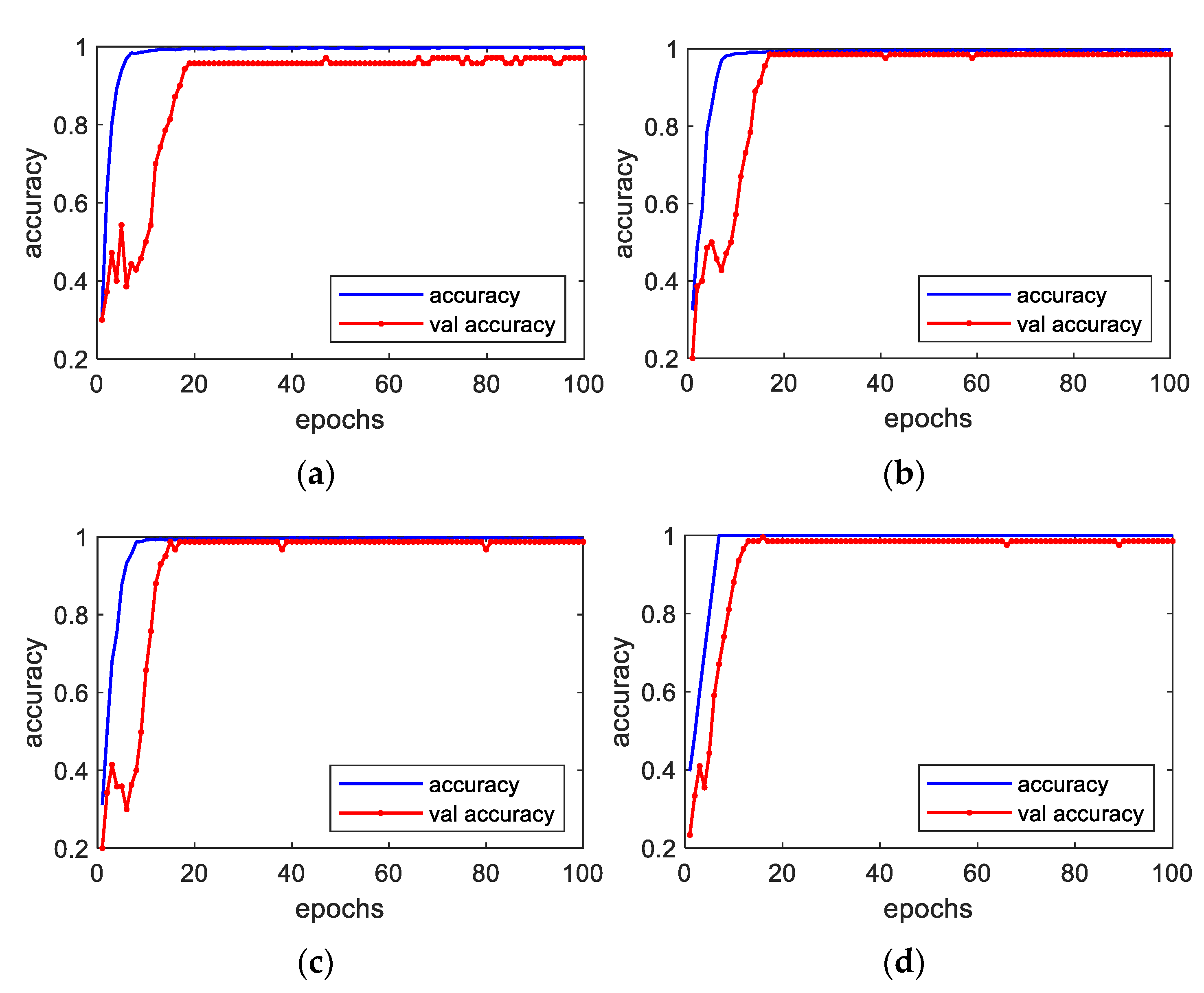
4.1.2. Diagnostic Results under Steady Conditions

Using the above dataset, the SNDCNN was used to train and verify datasets A, B, C, and D. The number of iterations for each dataset was 100, and the recognition rate, loss function, and training time of the SNDCNN were output. The test results are shown in Figure 7 and Table 3. In the figure, accuracy represents the detection rate of the training set, and var accuracy represents the detection rate of the test set.
In order to verify the impact of switchable normalization on the model, we compared it with batch normalization, which is widely used in convolutional neural networks, and the experimental results are shown in Figure 8. The average fault detection rate of switchable normalization for the four datasets was 99.68%, which was better than the average fault detection rate of batch normalization of 97.78%.
To further verify the fault detection ability of the SNDCNN proposed in this paper, we compared it with several traditional machine-learning-based diagnostic methods and several deep-learning-based diagnostic methods. The following methods all used the CWRU bearing dataset, with the only differences being in the number of training and test sets. Therefore, the comparison could objectively reflect the advantages of the SNDCNN in terms of the fault detection rate. The specific comparison results are shown in Table 4.
To verify whether the SNDCNN classification ability was improved by increasing the number of training sets, t-SNE dimensionality reduction technology was used to visualize the corresponding SNDCNN classification results when the number of training sets was 120, 1200, 3000, and 24,000, as shown in Figure 9. The results showed that the data enhancement of the training set could effectively improve the SNDCNN detection effect.

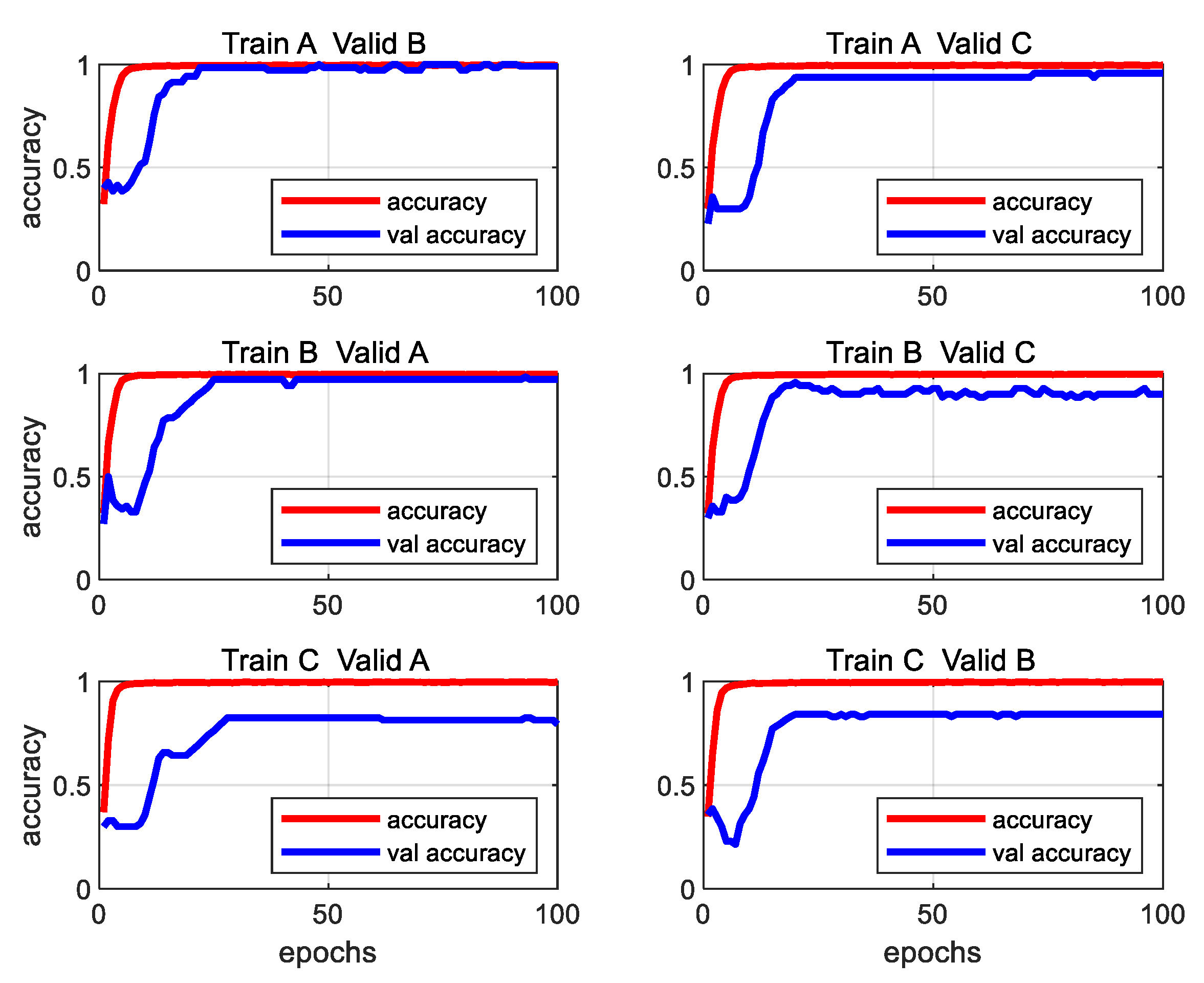
4.1.3. Diagnostic Results under Variable Load Conditions

In actual applications, machines often work under different operating loads. Such a complex working environment elicits higher requirements for fault diagnosis models. Neural networks trained under one load often cannot handle another load. To verify the fault detection rate of the SNDCNN under different loads, the SNDCNN was trained by the vibration data under 1 hp (dataset A), 2 hp (dataset B), and 3 hp (dataset C), where 1 hp, 2 hp, and 3 hp correspond to the speeds of 1772 r/min, 1750 r/min, and 1730 r/min, respectively. Figure 10 shows the data under different operating loads.
Figure 10 shows the ball fault signal with a fault level of 0.007 inches under different loads. It can be seen that the amplitude of the fault signal varied under different loads.
The experiment used the signals under one load as the training set and the signals under the other two loads as the test set for testing. The test results are shown in Figure 11 and Table 5.
The results showed that the SNDCNN had a detection rate of more than 90% under different loads, and the average training time of each signal was about 0.693 ms. Therefore, the SNDCNN had strong adaptability across load domains and could complete fault diagnosis tasks in complex and changing operating environments.

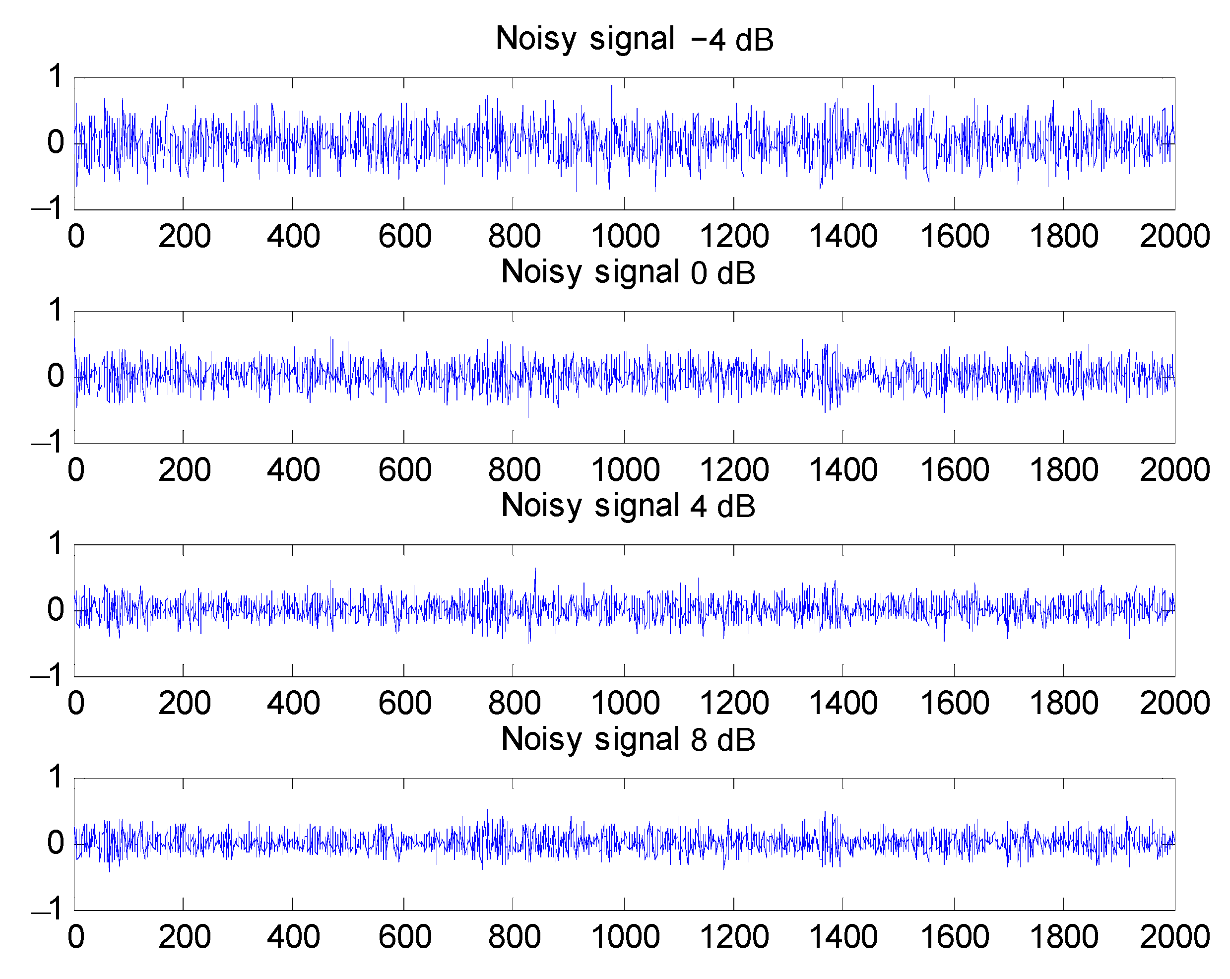
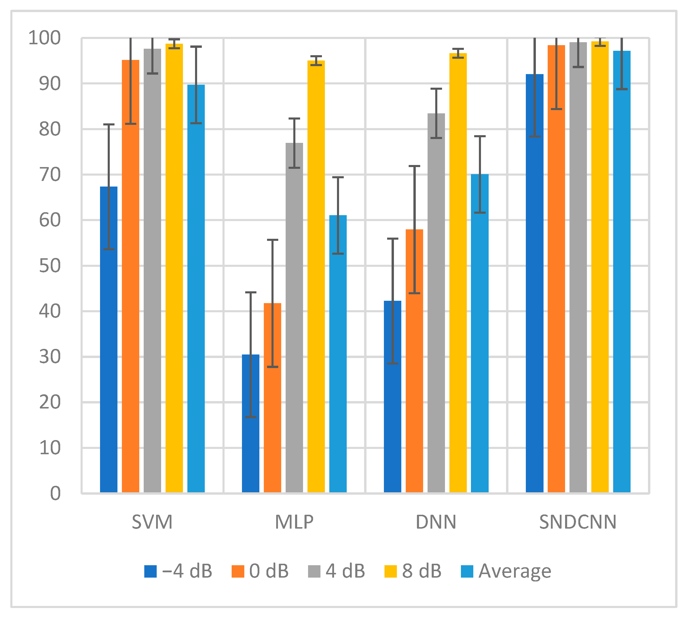
4.1.4. Diagnostic Results under Different Noise Conditions

To show that the SNDCNN had a high anti-noise performance, we also studied the diagnostic effect of the SNDCNN under different noise environments by introducing the concept of the signal-to-noise ratio (SNR), which is the ratio of useful signal power to noise power. The SNR is an important criterion for evaluating the strength of noise for a signal. The calculation formula of the SNR is as follows:
S N R dB = 10 log 10 P s i g n a l P n o i s e = 20 log 10 A s i g n a l A n o i s e
where Psignal is the signal power; Pnoise is the noise power; Asignal is the signal amplitude; and Anoise is the noise amplitude.
Environmental noise of different intensities has different effects on the raw vibration signal and may cover up the fault information of the raw vibration signal, making the SNDCNN unable to diagnose the fault well. Figure 12 shows the results of adding SNRs of −4 dB, 0 dB, 4 dB, and 8 dB Gaussian white noise to the raw vibration signal.
At this stage, the SNDCNN was trained by four vibration datasets with noise to test its detection rate at different noise intensities, and the diagnosis results were compared with support vector machines, multi-layer perceptrons (MLPs), and deep neural networks in the same noise environment. The average detection rate under the four different noise environments was calculated. The results of the average detection rate are shown in Table 6 and Figure 13. The results showed that the detection rate of the SNDCNN model in the four different noise environments was significantly higher than that of the other three diagnostic models, and the average detection rate was 97.15%, demonstrating a high anti-noise performance.

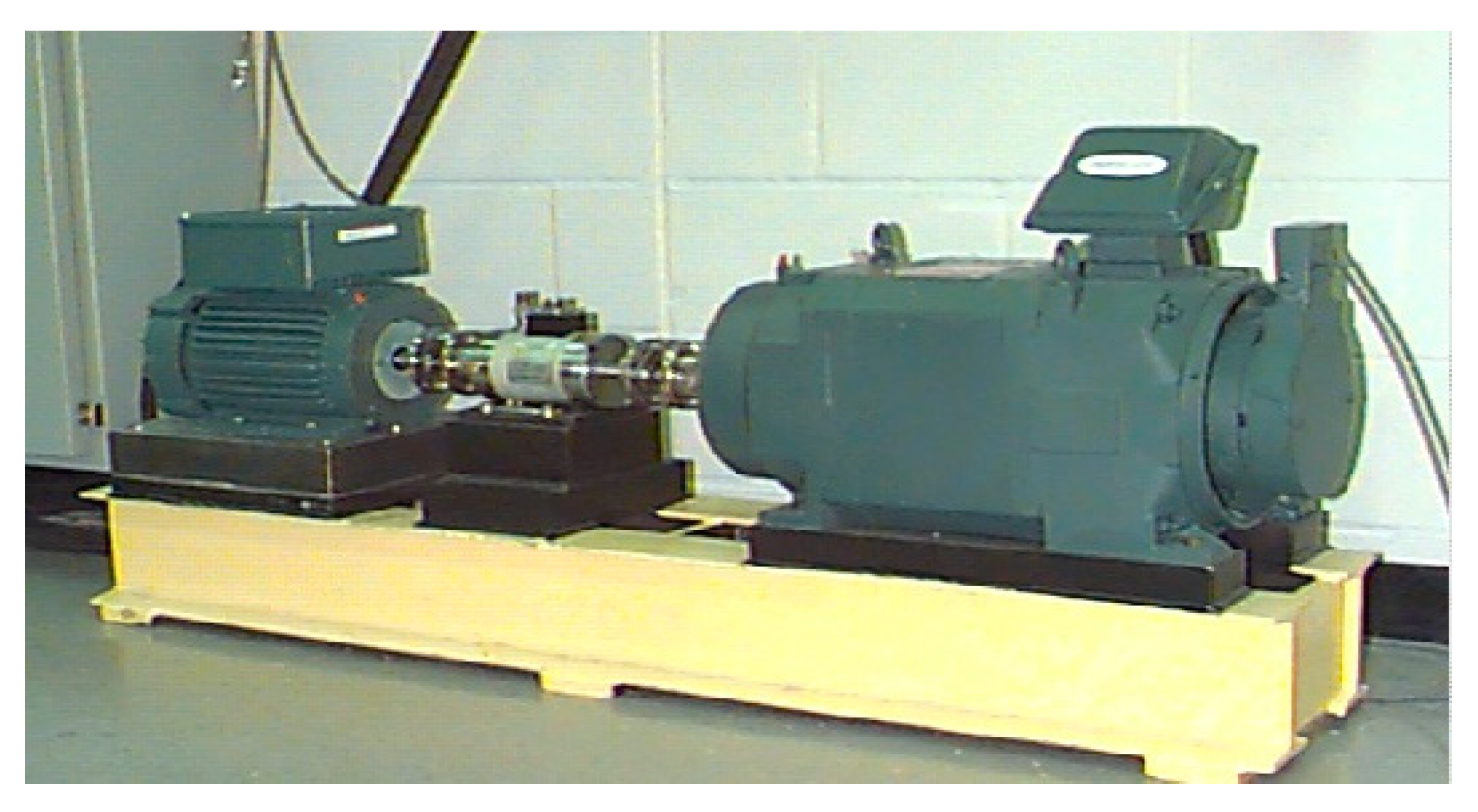
4.2. Case 2—Rolling Bearing Test Platform Data Analysis

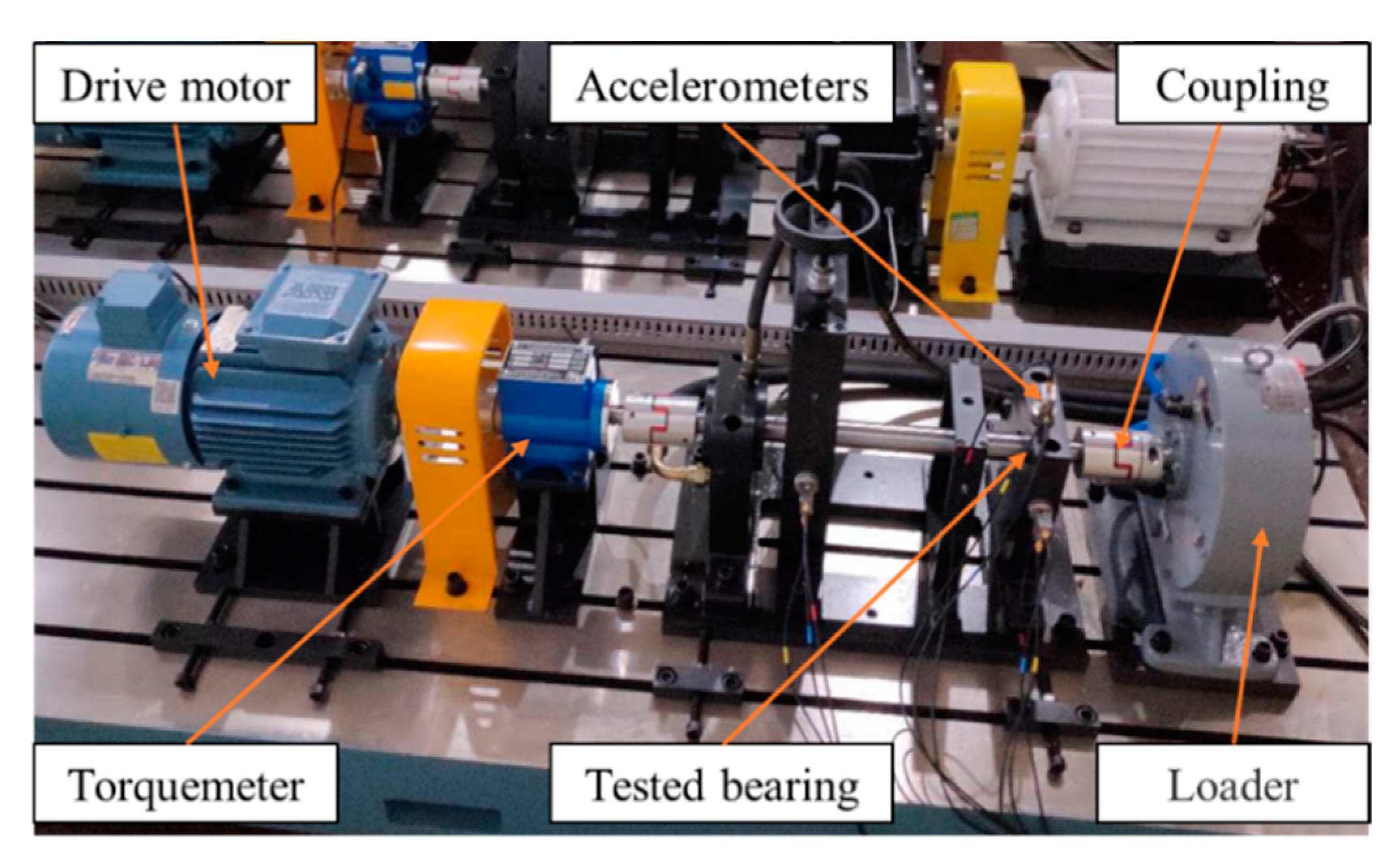
4.2.1. Test Bench Description

Figure 14 displays the rolling bearing test platform, which consisted of several parts. This test platform could conduct fault simulation tests of bearings under different operating conditions. The adjustable operating conditions of the test platform mainly included speed and load. The test bearing was a TPI6205 rolling bearing, and three fault forms of the ball, inner ring, and outer ring were processed by laser pitting. The specific parameters of the rolling bearings are shown in Table 7. Figure 15 shows photographs of the normal and faulted bearings. To collect vibration signals from the tested bearings, as shown in Figure 13, the accelerometer of type HD-YD-232 was positioned on the housing of the tested bearings, and the sampling frequency was set to 12 kHz.
The rolling bearing test bench was designed for experiments with different bearing failure degrees, different loads, different speeds, and a constant speed acceleration. We saved the experimental data to a series of files and filled in the file names with sequential numbers. The non-constant speed acceleration experiment stopped when the file size exceeded 16,384 KB, and the constant speed acceleration experiment stopped when the specified speed was reached. Taking the minor fault of the inner ring as an example, the details of the data records are shown in Table 8. Load 0 corresponded to operation under the no-load state, load 1 corresponded to a loading of 0.5 N∙m, load 2 corresponded to a loading of 1 N∙m, and load 3 corresponded to a loading of 1.5 N∙m.

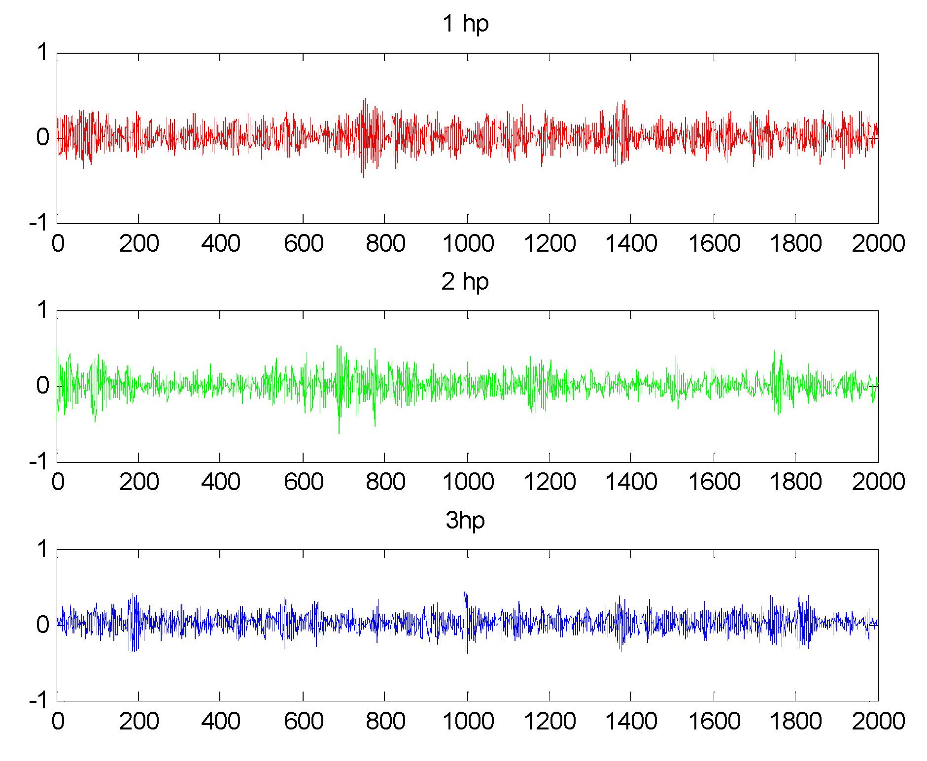
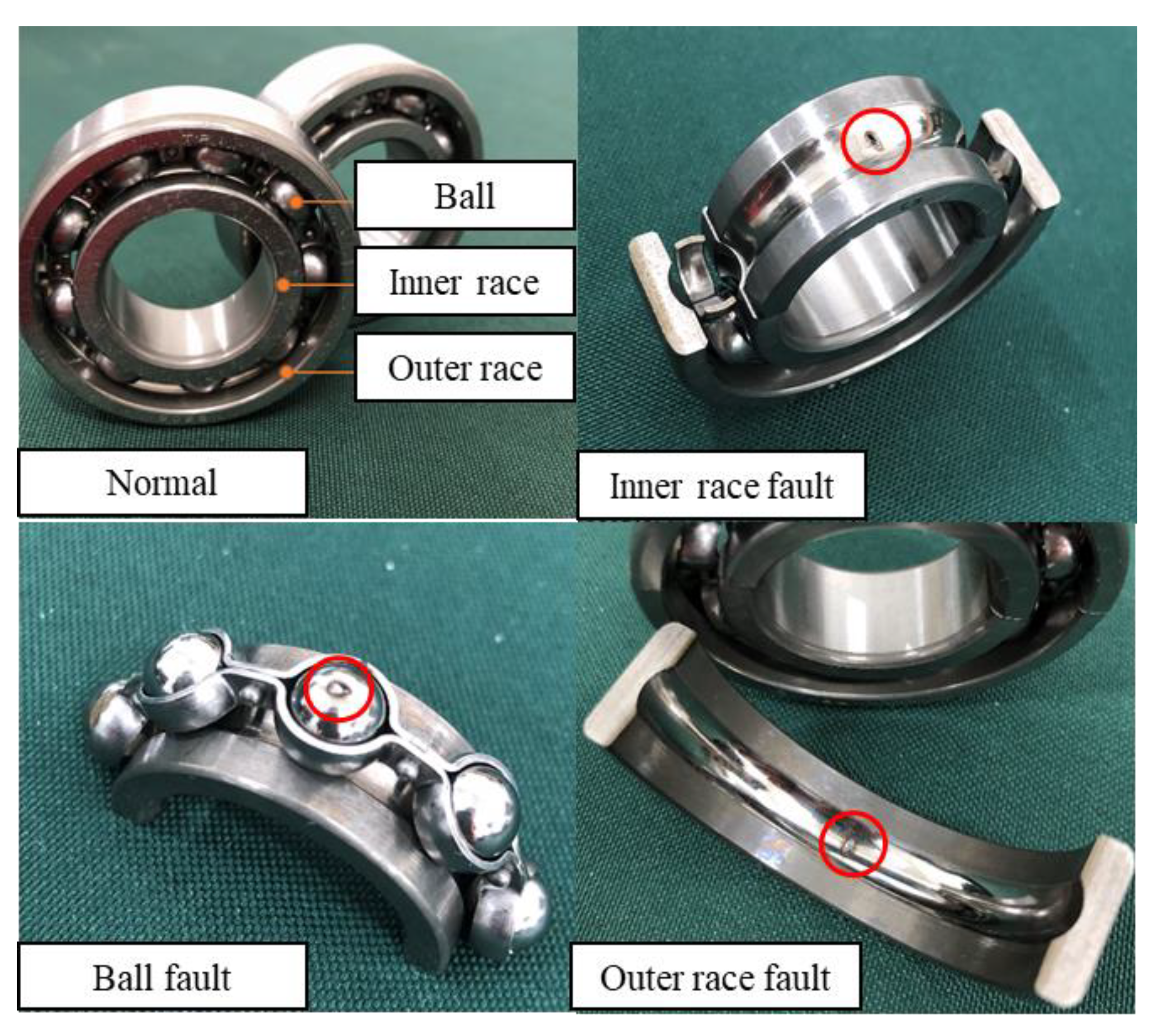
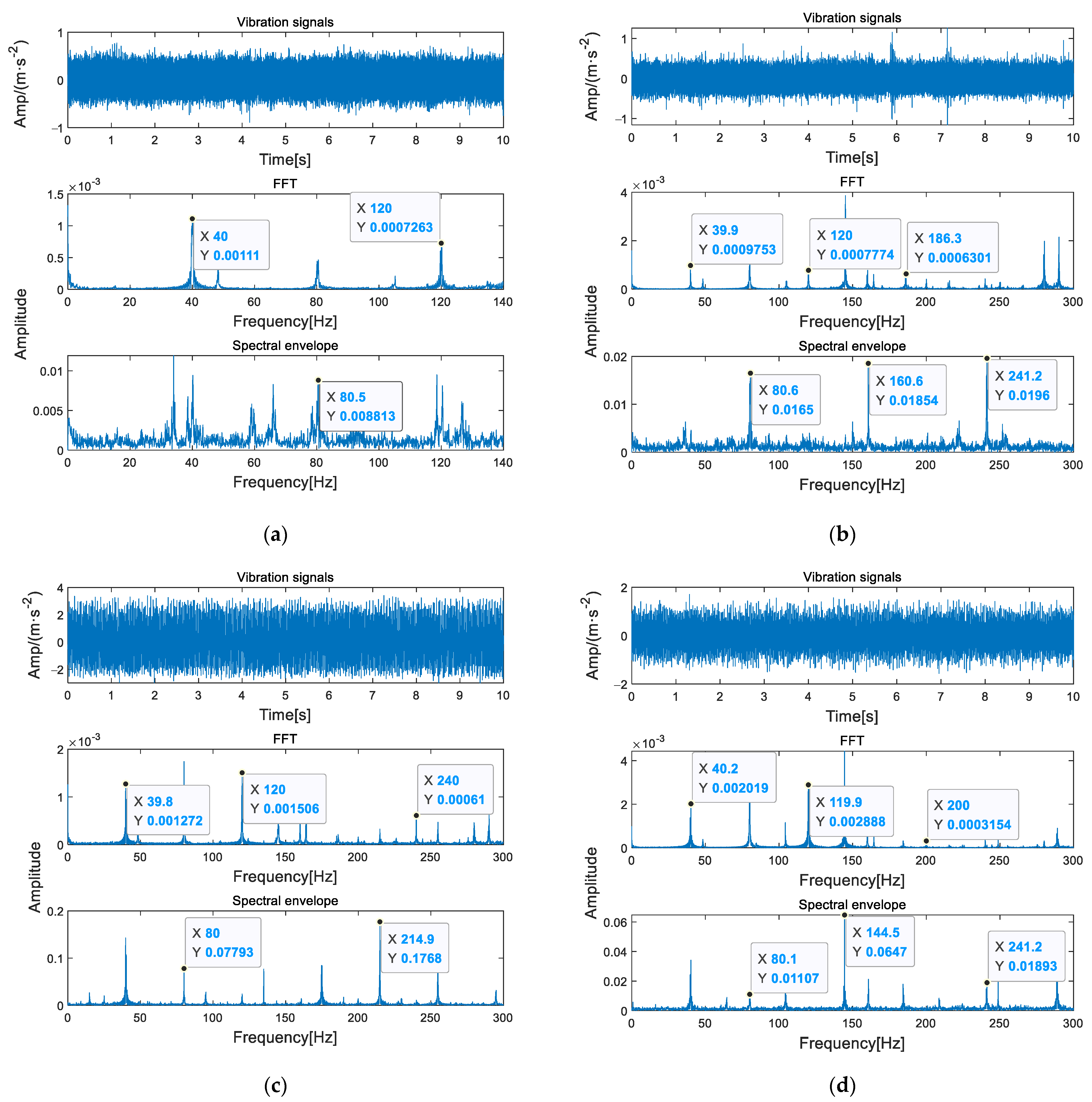
4.2.2. Bearing Fault Forms and Vibration Signal Analysis

We selected four bearing types under the conditions of rotating speed n = 2400 r/min and 0 loads and drew their original time domain signal, frequency spectrum, and envelope spectrum, as shown in Figure 16.
As shown in Figure 15, in addition to 40 Hz and the frequency component of doubling frequency, frequency components of 186.3 Hz, 214.9 Hz, and 144.5 Hz appeared in the spectrum and envelope spectrum, which were close to the theoretical values of the corresponding fault characteristic frequencies of 188.54 Hz, 216.6 Hz, and 143.39 Hz, respectively.
Through the observation and analysis of the original time domain signals, spectra, and envelope spectra of the above four conditions, obvious frequency doubling characteristics could be seen in the time spectra of the four types of signals, with the inner ring faults, outer ring faults, and ball faults all having obvious characteristic frequencies. Therefore, the overall design of the rolling bearing fault diagnosis test bed at this stage of the study was reasonable and could effectively simulate the damage of rolling bearings in different positions.

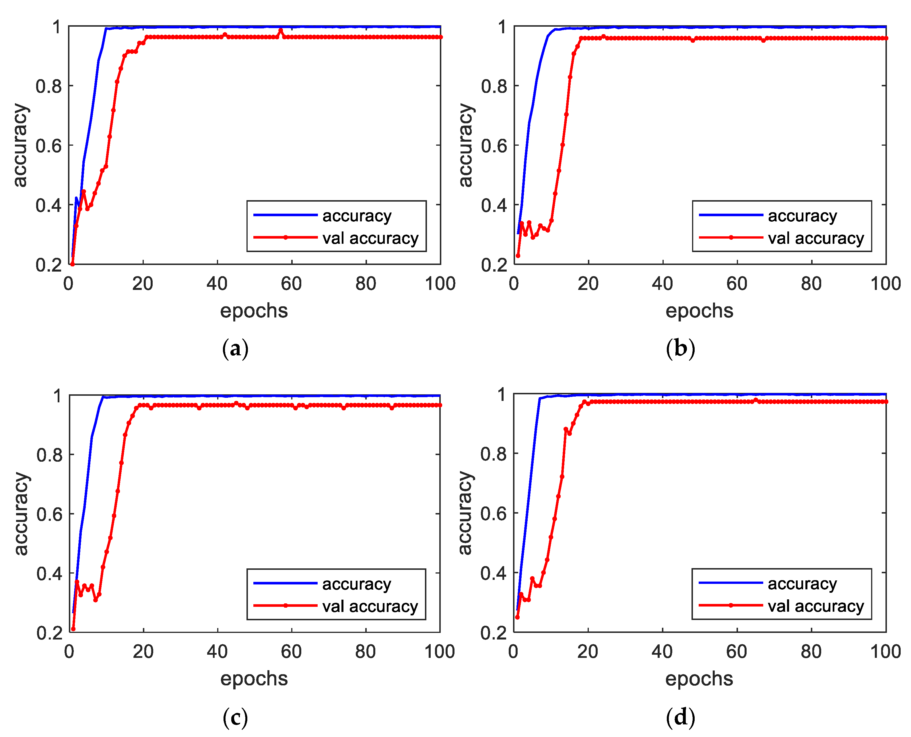
4.2.3. Diagnostic Results under Steady Conditions

In the case of a single load, the bearing was diagnosed with a total of three damage positions, on the rolling body of the bearing, the inner ring, and the outer ring. The damage degree was divided into three types, mild, moderate, and severe, and with the data of the bearing in a healthy state, this made up a total of 10 operating states. The speed was 2400 rpm/min.
At this stage, we expanded upon the data of the training set by employing overlapping sampling, that is, starting from the initial sampling point, the data length of each sample was N, and the location of the next sample was offset by N from that of the previous one. During the neural network training, N data points were trained each time. In this section, the length of the sampled data was 2048, and the offset length of the sampling position was 64. The specific division of the experimental dataset is shown in Table 9.
The trained fault diagnosis model was used to verify the divided single-load datasets. The number of iterations was 100, and the experiment was repeated 10 times. The diagnostic results are shown in Figure 17.
It can be seen from Figure 17 that the model could quickly converge, and the diagnosis rate under each load reached more than 97%, with the diagnosis rate for the dataset with load 3 being the highest at 98.71%. The experimental results showed that the model had high diagnostic accuracy under a single load. The results of the experiment are shown in Table 10.

4.2.4. Diagnosis Results under Variable Speed Conditions

In real industrial activities, bearings often work by accelerating or, in some cases, decelerating; the bearing fault diagnosis experimental platform designed in this study also simulated this situation. The control unit of the experimental platform was used to set the constant speed acceleration of the bearings. Two accelerations were set, 40 rpm/s and 80 rpm/s, to increase the running speed of the bearing from 800 rpm/min to 3200 rpm/min, respectively, and the recording times were about 1 min and 30 s.
The experimental data for a constant speed acceleration of 40 rpm/s were used in the experiment described in this section. Under these conditions, there were three fault types among the bearings, namely rolling body faults, inner ring faults, and outer ring faults. Each fault type comprised three degrees of damage. Including the running data of the bearings in a healthy state, there were a total of 10 operating states, and each damage degree comprised 300 training samples and 70 test samples. The training set adopted the method of overlapping sampling, with a sampling length of 2048 and a sampling location offset length of 128, while the test set did not adopt the method of overlapping sampling. Dataset A is the data collected under load 0, and datasets B, C, and D correspond to the data collected under loads 1, 2, and 3, respectively. The division of the experimental dataset is shown in Table 11.
The trained fault diagnosis model was verified using the fixed and rising speed dataset with 100 iterations. The diagnostic results are shown in Figure 18.
It can be observed from Figure 18 that the model could quickly converge, and the diagnostic rate of the constant speed and acceleration datasets under each load reached more than 95%, with high diagnostic accuracy. The experimental results showed that the proposed method could achieve high diagnostic accuracy under the conditions of a constant and increasing bearing speed. The results of the experiment are shown in Table 12.

5. Conclusions

In this paper, a fault diagnosis method for rolling bearings based on the SNDCNN method was studied, and the following conclusions were drawn:
  • The SNDCNN model, applicable to complex operating conditions, could directly input the raw vibration signal, and the fault detection rate reached 99.45% under multiple operating conditions.
  • The method of increasing the convolution kernel width of the first layer and multi-layer convolution kernel stacking could effectively extract fault features and suppress high-frequency noise.
  • The pooling operation of K-max pooling was used in the pooling layer, which could effectively retain the strong feature information.
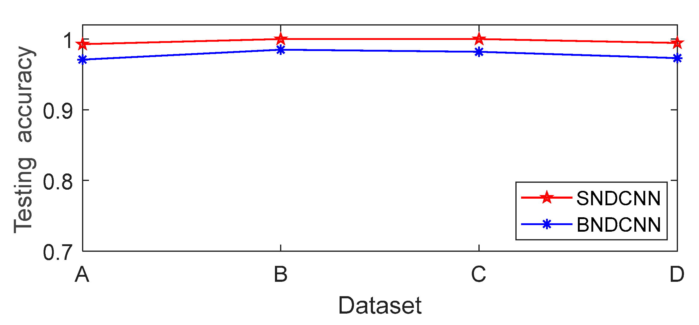
  • Each convolutional layer and fully connected layer adopted a switchable normalization method, which could effectively suppress overfitting and improve the model’s generalization performance.

Author Contributions

Conceptualization, X.H. and Y.C.; methodology, X.H. and Y.C.; software, X.H.; validation, J.L. and R.A.; formal analysis, W.F.; investigation, S.L.; resources, Y.C.; data curation, J.L.; writing—original draft preparation, X.H.; writing—review and editing, Y.C.; visualization, R.A.; supervision, W.F.; project administration, S.L.; funding acquisition, Y.C. All authors have read and agreed to the published version of the manuscript.

Funding

This research was funded by the National Science and Technology Major Project of China (J2019-I-0003-0004).

Data Availability Statement

Not applicable.

Conflicts of Interest

The authors declare no conflict of interest.

Nomenclature

SymbolDescription
SNswitchable normalization
DCNNdeep convolutional neural network
SVMsupport vector machine
CNNconvolutional neural network
DTSdislocated time series
INinstance normalization
LNlayer normalization
BNbatch normalization
GNgroup normalization
Adamadaptive momentum
CWRUCase Western Reserve University
EEMDensemble empirical mode decomposition
STFTshort-time Fourier transform
SNRsignal–noise ratio
MLPmulti-layer perceptron

References

  1. Ambrozkiewicz, B.; Syta, A.; Gassner, A.; Georgiadis, A.; Litak, G.; Meier, N. The influence of the radial internal clearance on the dynamic response of self-aligning ball bearings. Mech. Syst. Signal Process. 2022, 171, 108954–108964. [Google Scholar] [CrossRef]
  2. Liu, R.; Yang, B.; Enrico, Z.; Chen, X. Artificial intelligence for fault diagnosis of rotating machinery: A review. Mech. Syst. Signal Process. 2018, 108, 33–47. [Google Scholar] [CrossRef]
  3. Huang, W.; Gao, G.; Li, N.; Jiang, X.; Zhu, Z. Time-Frequency Squeezing and Generalized Demodulation Combined for Variable Speed Bearing Fault Diagnosis. IEEE Trans. Instrum. Meas. 2018, 8, 2819–2829. [Google Scholar] [CrossRef]
  4. Li, J.; Wang, H.; Wang, X.; Zhang, Y. Rolling bearing fault diagnosis based on improved adaptive parameterless empirical wavelet transform and sparse denoising. Measurement 2020, 152, 107392. [Google Scholar] [CrossRef]
  5. Guo, J.; Zhen, D.; Li, H.; Shi, Z.; Gu, F.; Andrew, D.B. Fault feature extraction for rolling element bearing diagnosis based on a multi-stage noise reduction method. Measurement 2019, 139, 226–235. [Google Scholar] [CrossRef] [Green Version]
  6. Wang, L.; Liu, Z.; Cao, H.; Zhang, X. Subband averaging kurtogram with dual-tree complex wavelet packet transform for rotating machinery fault diagnosis. Mech. Syst. Signal Process. 2020, 142, 106755. [Google Scholar] [CrossRef]
  7. Yu, K.; Lin, T.; Tan, J.; Ma, H. An adaptive sensitive frequency band selection method for empirical wavelet transform and its application in bearing fault diagnosis. Measurement 2019, 134, 375–384. [Google Scholar] [CrossRef]
  8. Cao, H.; Fan, F.; Zhou, K.; He, Z. Wheel-bearing fault diagnosis of trains using empirical wavelet transform. Measurement 2016, 82, 439–449. [Google Scholar] [CrossRef]
  9. Jiang, F.; Zhu, Z.; Li, W. An Improved VMD With Empirical Mode Decomposition and Its Application in Incipient Fault Detection of Rolling Bearin. IEEE Access 2018, 6, 44483–44493. [Google Scholar] [CrossRef]
  10. Yang, J.; Huang, D.; Zhou, D.; Liu, H. Optimal IMF selection and unknown fault feature extraction for rolling bearings with different defect modes. Measurement 2020, 157, 107660. [Google Scholar] [CrossRef]
  11. Li, J.; Yao, X.; Wang, H.; Zhang, J. Periodic impulses extraction based on improved adaptive VMD and sparse code shrinkage denoising and its application in rotating machinery fault diagnosis. Mech. Syst. Signal Process. 2019, 126, 568–589. [Google Scholar] [CrossRef]
  12. Li, J.; Meng, Z.; Yin, N.; Pan, Z.; Cao, L.; Fan, F. Multi-source feature extraction of rolling bearing compression measurement signal based on independent component analysis. Measurement 2020, 172, 108908. [Google Scholar] [CrossRef]
  13. Hu, Y.; Bao, W.; Tu, X.; Li, F.; Li, K. An Adaptive Spectral Kurtosis Method and Its Application to Fault Detection of Rolling Element Bearings. IEEE Trans. Instrum. Meas. 2019, 69, 739–750. [Google Scholar] [CrossRef]
  14. Udmale, S.S.; Singh, S.K. Application of Spectral Kurtosis and Improved Extreme Learning Machine for Bearing Fault Classification. IEEE Trans. Instrum. Meas. 2019, 68, 4222–4233. [Google Scholar] [CrossRef]
  15. Sohaib, M.; Kim, J. Fault Diagnosis of Rotary Machine Bearings Under Inconsistent Working Conditions. IEEE Trans. Instrum. Meas. 2019, 69, 3334–3347. [Google Scholar] [CrossRef]
  16. Jin, G.; Zhu, T.; Akram, M.W.; Jin, Y.; Zhu, C. An Adaptive Anti-Noise Neural Network for Bearing Fault Diagnosis Under Noise and Varying Load Conditions. IEEE Access 2020, 8, 74793–74807. [Google Scholar] [CrossRef]
  17. Qin, M.; Yan, S.; Tang, X.; Xu, C. Deep Convolutional and LSTM Recurrent Neural Networks for Rolling Bearing Fault Diagnosis Under Strong Noises and Variable Loads. IEEE Access 2020, 8, 66257–66269. [Google Scholar]
  18. Wang, Z.; Yao, L.; Cai, Y. Rolling bearing fault diagnosis using generalized refined composite multiscale sample entropy and optimized support vector machine. Measurement 2020, 156, 107574. [Google Scholar] [CrossRef]
  19. He, C.; Wu, T.; Liu, C.; Chen, T. A novel method of composite multiscale weighted permutation entropy and machine learning for fault complex system fault diagnosis. Measurement 2020, 158, 107748. [Google Scholar] [CrossRef]
  20. Yuan, H.; Wu, N.; Chen, X.; Wang, Y. Fault diagnosis of rolling bearing based on shift invariant sparse feature and optimized support vector machine. Machines 2021, 9, 98. [Google Scholar] [CrossRef]
  21. Wan, L.; Gong, K.; Zhang, G.; Yuan, X.; Li, C.; Deng, X. An Efficient Rolling Bearing Fault Diagnosis Method Based on Spark and Improved Random Forest Algorithm. IEEE Access 2021, 9, 37866–37882. [Google Scholar] [CrossRef]
  22. Chen, F.; Cheng, M.; Tang, B.; Chen, B.; Xiao, W. Pattern recognition of a sensitive feature set based on the orthogonal neighborhood preserving embedding and adaboost_SVM algorithm for rolling bearing early fault diagnosis. Meas. Sci. Technol. 2020, 31, 105007. [Google Scholar] [CrossRef]
  23. Li, J.; Yao, X.; Wang, X.; Yu, Q.; Zhang, Y. Multiscale local features learning based on BP neural network for rolling bearing intelligent fault diagnosis. Measurement 2020, 153, 107419. [Google Scholar] [CrossRef]
  24. Wang, G.; Luo, Z.; Qin, X.; Leng, Y.; Wang, T. Fault identification and classification of rolling element bearing based on time-varying autoregressive spectrum. Mech. Syst. Signal Process. 2008, 22, 934–947. [Google Scholar] [CrossRef]
  25. Liu, R.; Yang, B.; Hauptmann, A.G. Simultaneous Bearing Fault Recognition and Remaining Useful Life Prediction Using Joint-Loss Convolutional Neural Network. IEEE Trans. Ind. Inform. 2020, 16, 87–96. [Google Scholar] [CrossRef]
  26. Liu, H.; Zhou, J.; Zheng, Y.; Jiang, W.; Zhang, Y. Fault diagnosis of rolling bearings with recurrent neural network-based autoencoders. ISA Trans. 2018, 77, 167–178. [Google Scholar] [CrossRef] [PubMed]
  27. Xiang, Z.; Zhang, X.; Zhang, W.; Xia, X. Fault diagnosis of rolling bearing under fluctuating speed and variable load based on TCO Spectrum and Stacking Auto-encoder. Measurement 2019, 138, 162–174. [Google Scholar] [CrossRef]
  28. Meng, Z.; Zhan, X.; Li, J.; Pan, Z. An enhancement denoising autoencoder for rolling bearing fault diagnosis. Measurement 2018, 130, 448–454. [Google Scholar] [CrossRef] [Green Version]
  29. Kong, X.; Mao, G.; Wang, Q.; Ma, H.; Yang, W. A multi-ensemble method based on deep auto-encoders for fault diagnosis of rolling bearings. Measurement 2020, 151, 107132. [Google Scholar] [CrossRef]
  30. Xiao, Y.; Shao, H.; Han, S.; Huo, Z.; Wan, J. Novel Joint Transfer Network for Unsupervised Bearing Fault Diagnosis From Simulation Domain to Experimental Domain. IEEE-ASME Trans. Mechatron. 2022, 27, 5254–5263. [Google Scholar] [CrossRef]
  31. Lei, Y.; Yang, B.; Jiang, X.; Jia, F.; Li, N.; Nandi, A. Applications of machine learning to machine fault diagnosis: A review and roadmap. Mech. Syst. Signal Process. 2020, 138, 106587–106626. [Google Scholar] [CrossRef]
  32. Chen, X.; Wang, S.; Qiao, B.; Chen, Q. Basic research on machinery fault diagnostics: Past, present, and future trends. Front. Mech. Eng. 2018, 13, 264–291. [Google Scholar] [CrossRef] [Green Version]
  33. Guo, J.; Liu, X.; Li, S.; Wang, Z. Bearing Intelligent Fault Diagnosis Based on Wavelet Transform and Convolutional Neural Network. Shock Vib. 2020, 2020, 6380486. [Google Scholar] [CrossRef]
  34. He, F.; Ye, Q. A Bearing Fault Diagnosis Method Based on Wavelet Packet Transform and Convolutional Neural Network Optimized by Simulated Annealing Algorithm. Sensors 2022, 22, 1410. [Google Scholar] [CrossRef] [PubMed]
  35. Xiong, S.; Zhou, H.; He, S.; Zhang, L.; Xia, Q.; Xuan, J.; Shi, T. A Novel End-To-End Fault Diagnosis Approach for Rolling Bearings by Integrating Wavelet Packet Transform into Convolutional Neural Network Structures. Sensors 2020, 20, 17. [Google Scholar] [CrossRef]
  36. Guo, S.; Yang, T.; Gao, W.; Zhang, C. A novel fault diagnosis method for rotating machinery based on a convolutional neural network. Sensors 2018, 18, 1429. [Google Scholar] [CrossRef] [Green Version]
  37. Guo, S.; Yang, T.; Gao, W.; Zhang, C.; Zhang, Y. An intelligent fault diagnosis method for bearings with variable rotating speed based on pythagorean spatial pyramid pooling CNN. Sensors 2018, 18, 3857. [Google Scholar] [CrossRef] [Green Version]
  38. Sun, W.; Yao, B.; Zeng, N.; Chen, B.; He, Y.; Cao, X.; He, W. An intelligent gear fault diagnosis methodology using a complex wavelet enhanced convolutional neural network. Materials 2017, 10, 790. [Google Scholar] [CrossRef] [Green Version]
  39. Cao, X.; Chen, B.; Yao, B.; He, W. Combining translation-invariant wavelet frames and convolutional neural network for intelligent tool wear state identification. Comput. Ind. 2019, 106, 71–84. [Google Scholar] [CrossRef]
  40. Li, Z.; Zheng, T.; Yang, W.; Fu, H.; Wu, W. A Robust Fault Diagnosis Method for Rolling Bearings Based on Deep Convolutional Neural Network. In Proceedings of the 2019 Prognostics and System Health Management Conference, Qingdao, China, 25–27 October 2019; pp. 1–6. [Google Scholar]
  41. Han, T.; Liu, C.; Wu, L.; Sumik, S.; Jiang, D. An adaptive spatiotemporal feature learning approach for fault diagnosis in complex systems. Mech. Syst. Signal Process. 2018, 117, 170–187. [Google Scholar] [CrossRef]
  42. Zhang, Y.; Xing, K.; Bai, R.; Sun, D.; Meng, Z. An enhanced convolutional neural network for bearing fault diagnosis based on time–frequency image. Measurement 2020, 157, 107667. [Google Scholar] [CrossRef]
  43. Liu, R.; Meng, G.; Yang, B.; Sun, C.; Chen, X. Dislocated time series convolutional neural architecture: An intelligent fault diagnosis approach for electric machine. IEEE Trans. Ind. Inform. 2017, 13, 1310–1320. [Google Scholar] [CrossRef]
  44. Wen, L.; Li, X.; Gao, L.; Zhang, Y. A new convolutional neural network-based data-driven fault diagnosis method. IEEE Trans. Ind. Electron. 2018, 65, 5990–5998. [Google Scholar] [CrossRef]
  45. Zhou, P.; Zhou, G.; Zhu, Z.; Tang, C.; He, Z.; Li, W.; Jiang, F. Health monitoring for balancing tail ropes of a hoisting system using a convolutional neural network. Appl. Sci. 2018, 8, 1346. [Google Scholar] [CrossRef] [Green Version]
  46. Wang, H.; Xu, J.; Yan, R.; Gao, R. A New Intelligent Bearing Fault Diagnosis Method Using SDP Representation and SE-CNN. IEEE Trans. Instrum. Meas. 2020, 69, 2377–2389. [Google Scholar] [CrossRef]
  47. Shao, H.; Xia, M.; Han, G.; Zhang, Y.; Wang, J. Intelligent Fault Diagnosis of Rotor-Bearing System Under Varying Working Conditions With Modified Transfer Convolutional Neural Network and Thermal Images. IEEE Trans. Instrum. Meas. Info. 2021, 17, 3488–3496. [Google Scholar] [CrossRef]
  48. Chen, C.; Liu, Z.; Yang, G.; Wu, C.; Ye, Q. An Improved Fault Diagnosis Using 1D-Convolutional Neural Network Model. Electronics 2020, 10, 59. [Google Scholar] [CrossRef]
  49. Xue, Y.; Dou, D.; Yang, J. Multi-fault diagnosis of rotating machinery based on deep convolution neural network and support vector machine. Measurement 2020, 156, 107571. [Google Scholar] [CrossRef]
  50. Luo, P.; Zhang, R.; Ren, J.; Peng, Z.; Li, J. Switchable Normalization for Learning-to-Normalize Deep Representation. IEEE Trans. Pattern Anal. Mach. Intell. 2021, 43, 712–728. [Google Scholar] [CrossRef] [PubMed] [Green Version]
  51. Yao, D.; Yang, J.; Cheng, X.; Wang, X. Railway rolling bearing fault diagnosis based on muti-scale IMF permutation entropy and SA-SVM classifier. J. Mech. Eng. 2018, 54, 168–176. [Google Scholar] [CrossRef]
  52. Shen, Z.; Chen, X.; Zhang, X.; He, Z. A novel intelligent gear fault diagnosis model based on EMD and multi-class TSVM. Measurement 2012, 45, 30–40. [Google Scholar] [CrossRef]
  53. Zhao, Z.; Yang, S. Fault diagnosis of roller bearing based on relative wavelet energy. J. Electron. Meas. Instrum. 2011, 25, 44–49. [Google Scholar] [CrossRef]
  54. Zhang, C.; Feng, J.; Hu, C.; Liu, Z.; Cheng, L.; Zhou, Y. An Intelligent Fault Diagnosis Method of Rolling Bearing Under Variable Working Loads Using 1-D Stacked Dilated Convolutional Neural Network. IEEE Access 2020, 8, 63027–63042. [Google Scholar] [CrossRef]
Figure 1. Composition of CNN.
Machines 11 00185 g001
Figure 2. Pooling method comparison. The dotted lines in different colors represent pooling of different convolution filters.
Machines 11 00185 g002
Figure 3. Structure of SNDCNN.
Machines 11 00185 g003
Figure 4. The process flow of rolling bearing fault diagnosis based on SNDCNN.
Machines 11 00185 g004
Figure 5. The rolling bearing test rig.
Machines 11 00185 g005
Figure 6. Overlapping sampling process. The data in solid black represents the previous time of Overlapping sampling, and the data in dotted red represents the next time of Overlapping sampling.
Machines 11 00185 g006
Figure 7. The detection rate of the SNDCNN for the four datasets.
Machines 11 00185 g007
Figure 8. The detection rate of SNDCNN and BNDCNN for the four datasets.
Machines 11 00185 g008
Figure 9. t-SNE visualization results.
Machines 11 00185 g009
Figure 10. Ball fault signal under different loads.
Machines 11 00185 g010
Figure 11. The detection rate of the SNDCNN under different load conditions.
Machines 11 00185 g011
Figure 12. Vibration signals under different noise environments.
Machines 11 00185 g012
Figure 13. Comparison of diagnostic rates between SNDCNN and other fault diagnosis models under different noise environments.
Machines 11 00185 g013
Figure 14. A testbed of rolling element bearings.
Machines 11 00185 g014
Figure 15. The rolling bearings under four different conditions. The circle is the point of failure.
Machines 11 00185 g015
Figure 16. The rolling bearings under four different conditions: (a) normal; (b) ball fault; (c) inner race fault; (d) outer race fault.
Machines 11 00185 g016
Figure 17. The detection rate of the experiment: (a) dataset A; (b) dataset B; (c) dataset C; (d) dataset D.
Machines 11 00185 g017
Figure 18. The detection rate of the experiment: (a) dataset A; (b) dataset B; (c) dataset C; (d) dataset D.
Machines 11 00185 g018
Table 1. Structural parameters of SNDCNN.
No.Layer TypeSizeStrideKernel NumberPadding (Yes or No)
1C180 × 18*18Y
2P14 × 12*116N
3C25 × 11*132Y
4P22 × 12*132N
5C33 × 11*164Y
6P32 × 12*164N
7C43 × 11*164Y
8P42 × 12*164N
9C53 × 11*164Y
10P52 × 12*164N
11C63 × 11*164Y
12P62 × 12*164N
13F11001001N
14Softmax10101N
Table 2. Division of rolling bearing data.
Fault LocationNoneBallInner RaceOuter RaceLoad (hp)
Labels0123456789
Fault Diameter (inches)00.0070.0140.0210.0070.0140.0210.0070.0140.021
ATraining8008008008008008008008008008001
Testing40404040404040404040
Validation20202020202020202020
BTraining8008008008008008008008008008002
Testing40404040404040404040
Validation20202020202020202020
CTraining8008008008008008008008008008003
Testing40404040404040404040
Validation20202020202020202020
DTraining24002400240024002400240024002400240024001,2,3
Testing120120120120120120120120120120
Validation60606060606060606060
Table 3. SNDCNN diagnosis results.
Detection RateLoss FunctionTime (ms/step)Iterations
Dataset A99.27%0.0610.653100
Dataset B100.00%0.0540.749100
Dataset C100.00%0.0110.671100
Dataset D99.45%0.0630.687100
Table 4. Comparison of test results of different diagnostic methods.
Diagnosis
Method
Accuracy (%)
Dataset ADataset BDataset CDataset D
EEMD + SVM [51]92.2593.1692.5687.25
STFT + SVM [52]94.7693.5595.0586.39
WT + BP [53]93.6592.1494.8584.27
BPNN [54]62.11
MSCNN [54]98.46
DTS-CNN [54]99.14
1D-DCNN [54]98.43
SNDCNN99.27100.00100.0099.45
Table 5. Diagnostic results of the SNDCNN under different load conditions.
Detection RateLoss FunctionTime (ms/step)Iterations
A→B99.18%0.1010.674100
A→C95.72%0.4310.703100
B→A97.14%0.3720.689100
B→C90.00%0.6240.683100
C→A79.40%3.1950.714100
C→B84.15%0.9610.692100
Average90.93%0.9470.693100
Table 6. Diagnostic results of SNDCNN under different noise environments.
SVMMLPDNNSNDCNN
−4 dB67.3530.4842.2492.05
0 dB95.1541.7557.9398.37
4 dB97.6276.9383.4599.03
8 dB98.7395.0296.6499.25
Average89.712561.04570.06597.175
Table 7. TPI6205 rolling bearing parameters.
TypeDiameter of the BallPitch DiameterBall NumberContact Angle
TPI62050.3126 inches1.537 inches90
Table 8. Details of the data records.
FilenameLoadRotational
Speed (rpm)
FilenameLoadRotational
Speed (rpm)
Comment
Test_0010800Test_0133800
Test_00201600Test_01431600
Test_00302400Test_01532400
Test_00403200Test_01633200
Test_0051800Test_0170raising speed 40 rpm/s800 to 3200 rpm
Test_00611600Test_0180raising speed 80 rpm/s800 to 3200 rpm
Test_00712400Test_0191raising speed 40 rpm/s800 to 3200 rpm
Test_00813200Test_0201raising speed 80 rpm/s800 to 3200 rpm
Test_0092800Test_0212raising speed 40 rpm/s800 to 3200 rpm
Test_01021600Test_0222raising speed 80 rpm/s800 to 3200 rpm
Test_01122400Test_0233raising speed 40 rpm/s800 to 3200 rpm
Test_01223200Test_0243raising speed 80 rpm/s800 to 3200 rpm
Table 9. The specific division of the experimental dataset.
Fault LocationNoneBallInner RaceOuter RaceLoad
Labels0123456789
Fault DegreeNoneMildModerateSevereMildModerateSevereMildModerateSevere
ATraining8008008008008008008008008008000
Testing40404040404040404040
BTraining8008008008008008008008008008001
Testing40404040404040404040
CTraining8008008008008008008008008008002
Testing40404040404040404040
DTraining8008008008008008008008008008003
Testing40404040404040404040
Table 10. The results of the experiment.
Detection RateLoss FunctionTime (ms/step)Iterations
Dataset A97.14%0.0830.638100
Dataset B98.57%0.0690.726100
Dataset C98.71%0.0670.645100
Dataset D99.52%0.0690.633100
Table 11. The division of the experimental dataset.
Fault LocationNoneBallInner RaceOuter RaceLoad
Labels0123456789
Fault DegreeNoneMildModerateSevereMildModerateSevereMildModerateSevere
ATraining3003003003003003003003003003000
Testing70707070707070707070
BTraining3003003003003003003003003003001
Testing70707070707070707070
CTraining3003003003003003003003003003002
Testing70707070707070707070
DTraining3003003003003003003003003003003
Testing70707070707070707070
Table 12. The results of the experiment.
Detection RateLoss FunctionTime (ms/step)Iterations
Dataset A95.79%0.0890.652100
Dataset B95.33%0.0920.701100
Dataset C97.69%0.0810.633100
Dataset D98.52%0.0790.655100
Disclaimer/Publisher’s Note: The statements, opinions and data contained in all publications are solely those of the individual author(s) and contributor(s) and not of MDPI and/or the editor(s). MDPI and/or the editor(s) disclaim responsibility for any injury to people or property resulting from any ideas, methods, instructions or products referred to in the content.

