
Predictive Extended State Observer-Based Active Disturbance Rejection Control for Systems with Time Delay

Abstract
:1. Introduction
1.1. Related ADRC Works
1.2. Novelty and Contribution of This Paper
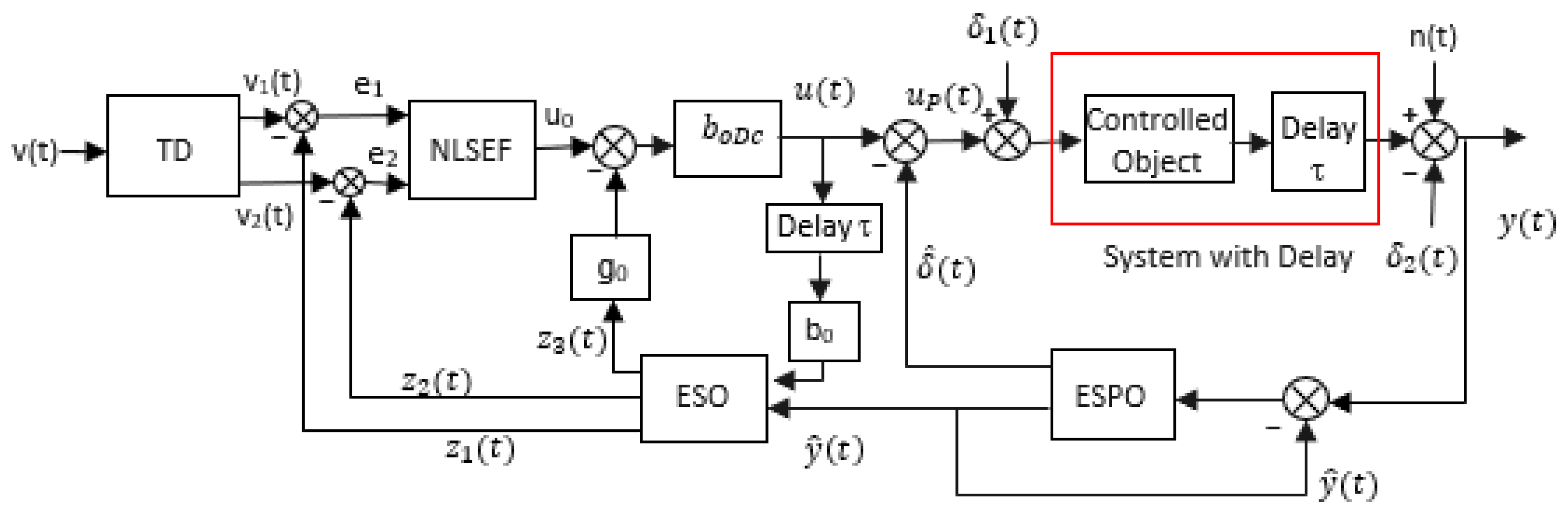
2. Preliminary Concepts Used in the Proposed Controller Design
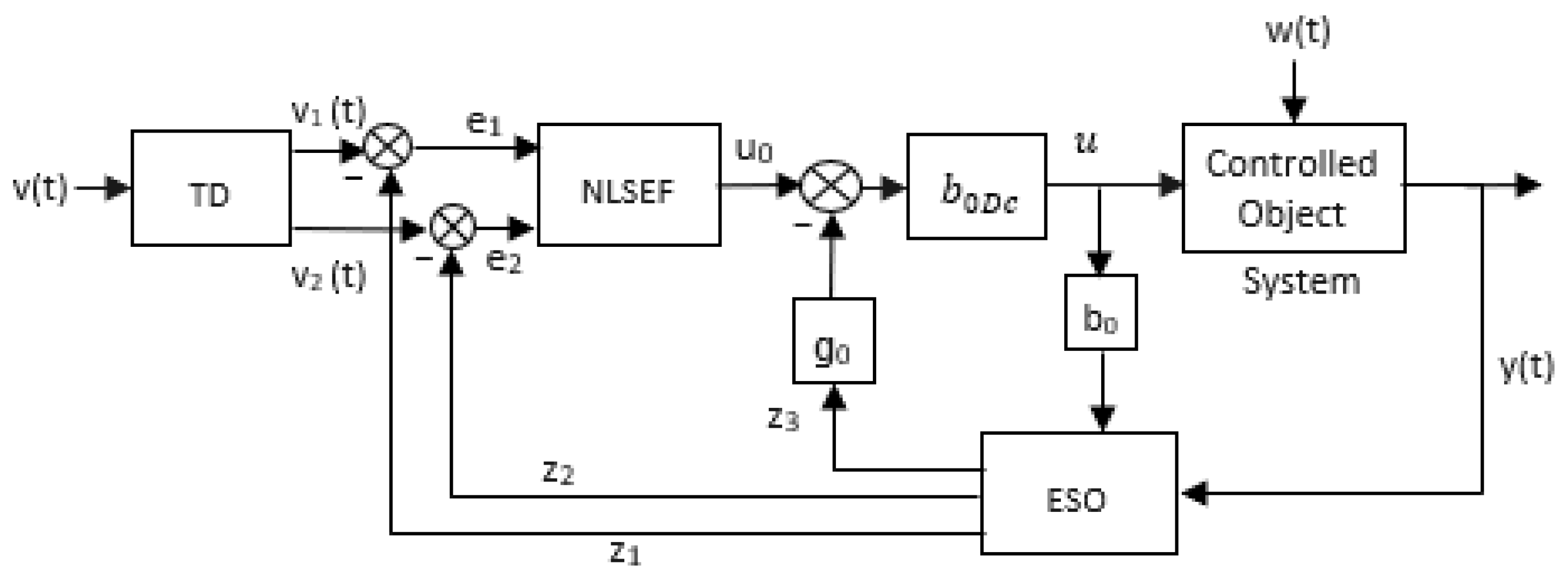
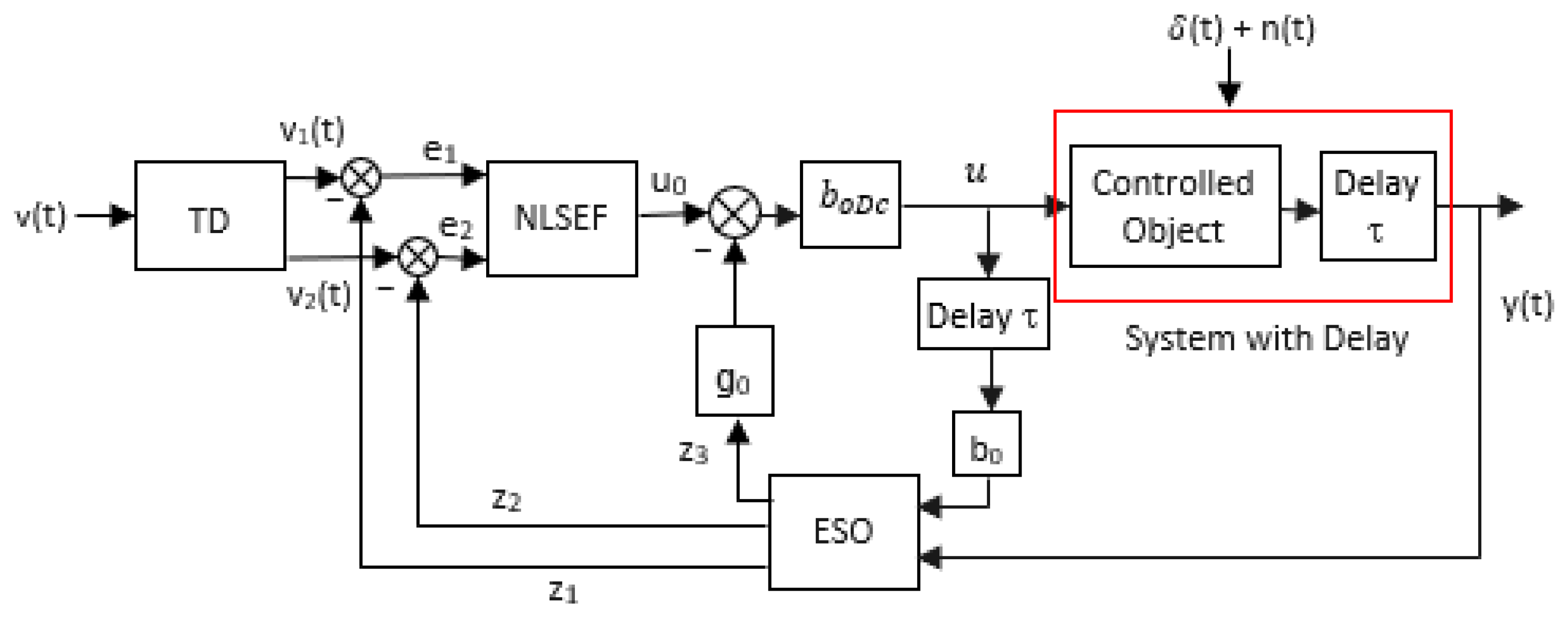
2.1. Conventional ADRC
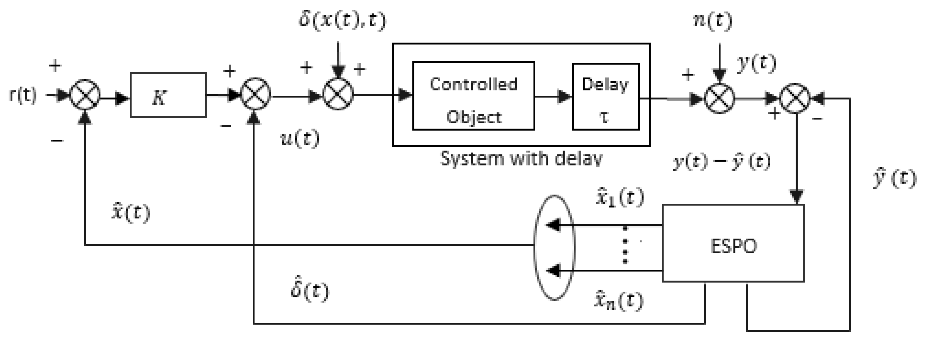
2.2. ESPO-Based Controller
2.3. Integral of Time-Weighted Absolute Error (ITAE) Criterion
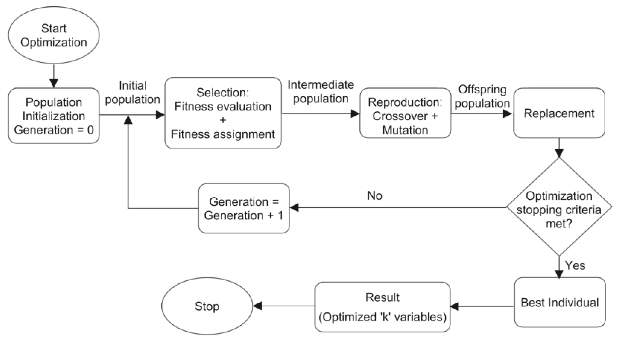
2.4. Optimizing the Controller Parameters using GA
3. Proposed Predictive ESO-based Active Disturbance Rejection Control Design
| Algorithm 1. Control Design of the Proposed Predictive ESO-based ADRC Controller | |
| 1: | Design the controller NLSEF of the modified time-delay-based ADRC structure: Use GA to find the optimal damping coefficient , the precision factor , and the control gain that minimizes the ITAE between the output response and the desired response. An automatic stop condition is incorporated. The optimization is conducted using the GA for Type 0 system given bounds on , , , , , and for a time-delay , whereas the optimization is conducted using the GA for Type 1 and Type 2 systems given bounds on , , and for a time-delay . , , , and for the ESO are kept constant. and for TD are kept constant. |
| 2: | if , , , , , or (for Type 0) value or , , or (for Type 1 and Type 2 systems) value falls on the bound after an optimization run then |
| 3: | bounds are changed and the ADRC is re-optimized. |
| 4: | Else |
| 5: | Save the best , , , , , and (for Type 0) or , , and (for Type 1 and Type 2 systems). |
| 6: | end if |
| 7: | Design the observer ESPO: Use Equations (11)–(14). The bandwidth is tuned to obtain the best disturbance compensation performance, given the input disturbances and output disturbance . |
| 8: | Obtain the control law ()) of the proposed controller design using Equation (19). |
| 9: | Simulate, with time-delay , the control of the plant by the proposed predictive ESO-based ADRC: The aim is to assess the proposed design’s controller performance for disturbance compensation in the presence of time delay. Keep the constants of ESPO found in line 7, delay-based ADRC constants, and NLSEF parameters found through the optimization in line 2 of Algorithm 1, with the input disturbances and output disturbance , and measurement noise . |
4. Experiments and Results
- (1)
- Modified time-delay-based ADRC:
- (2)
- ESPO-based controller:
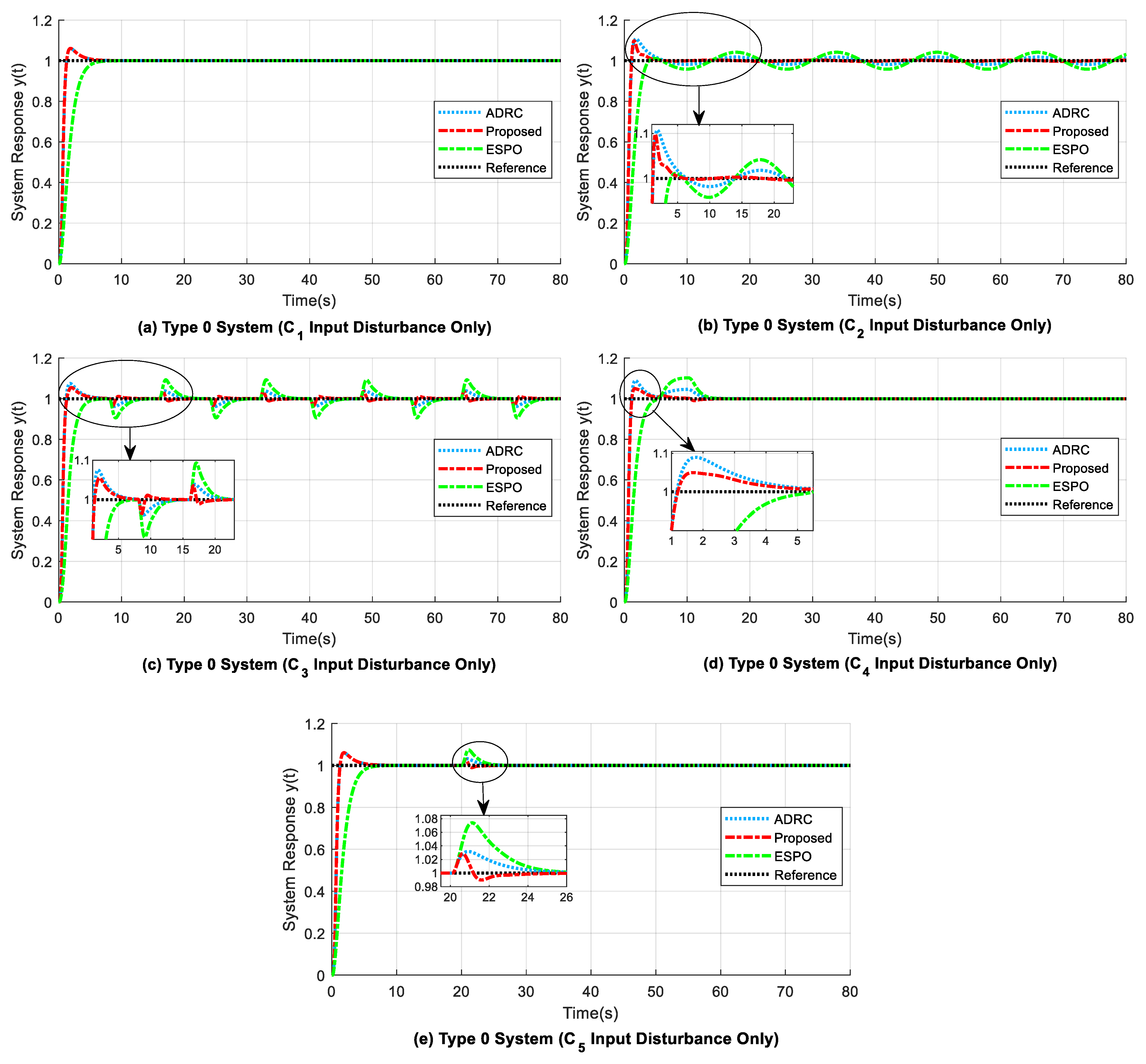
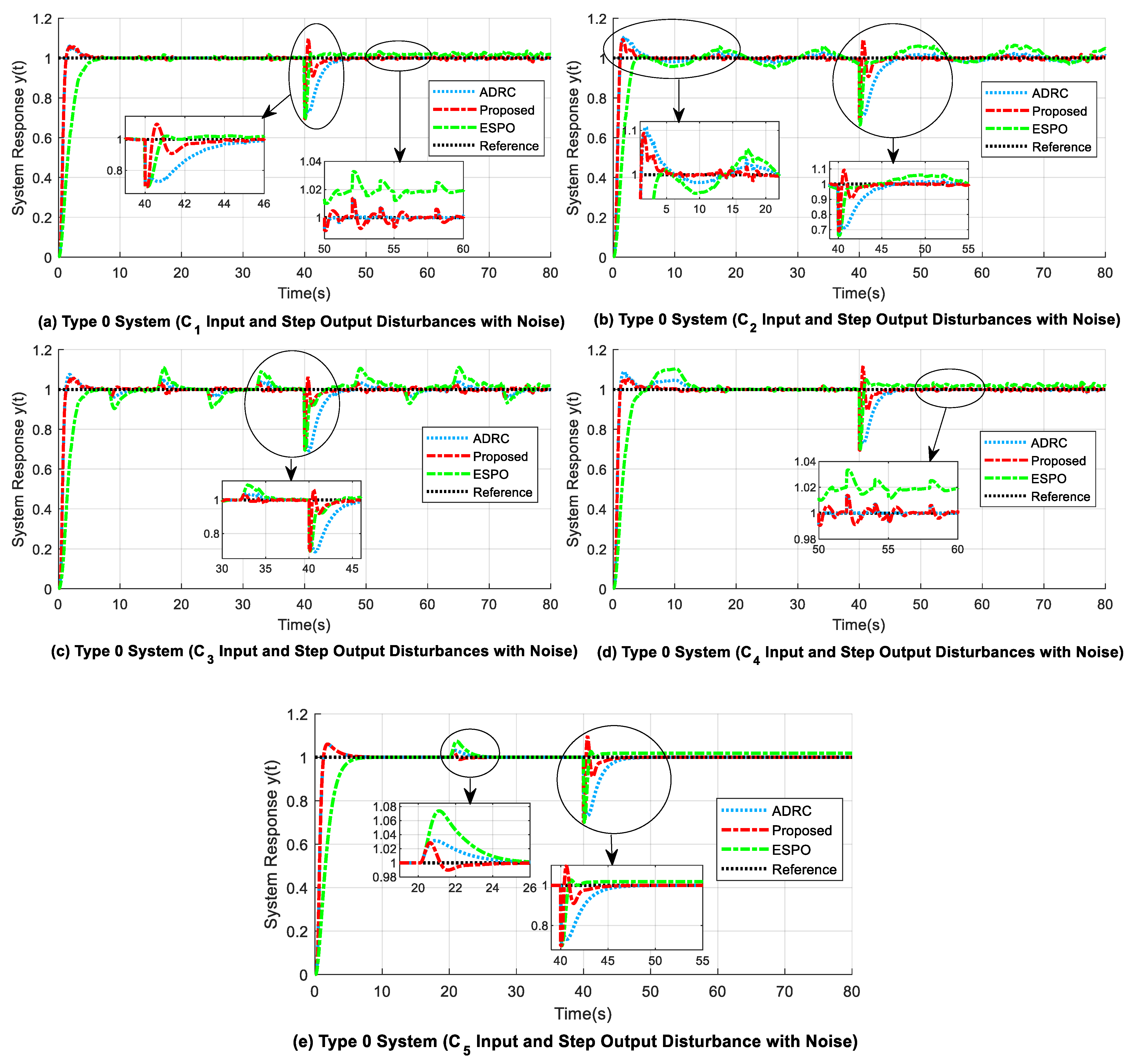
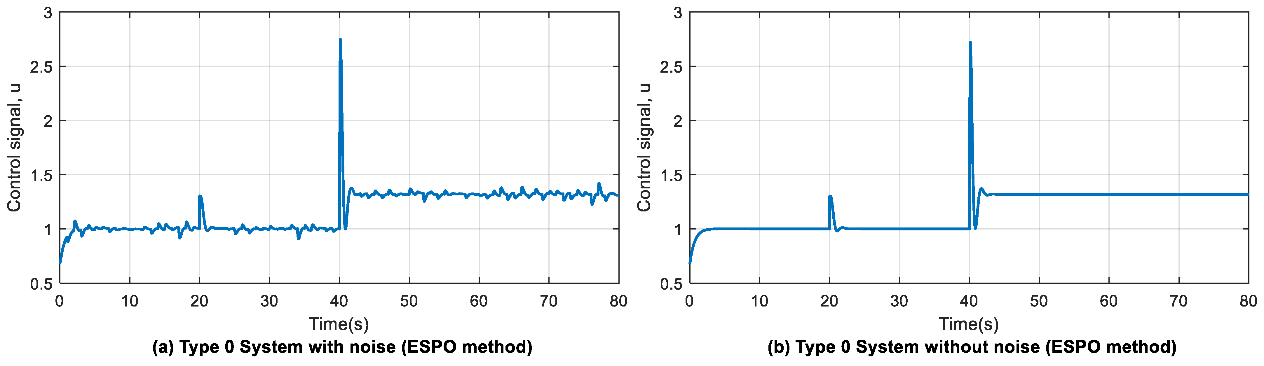
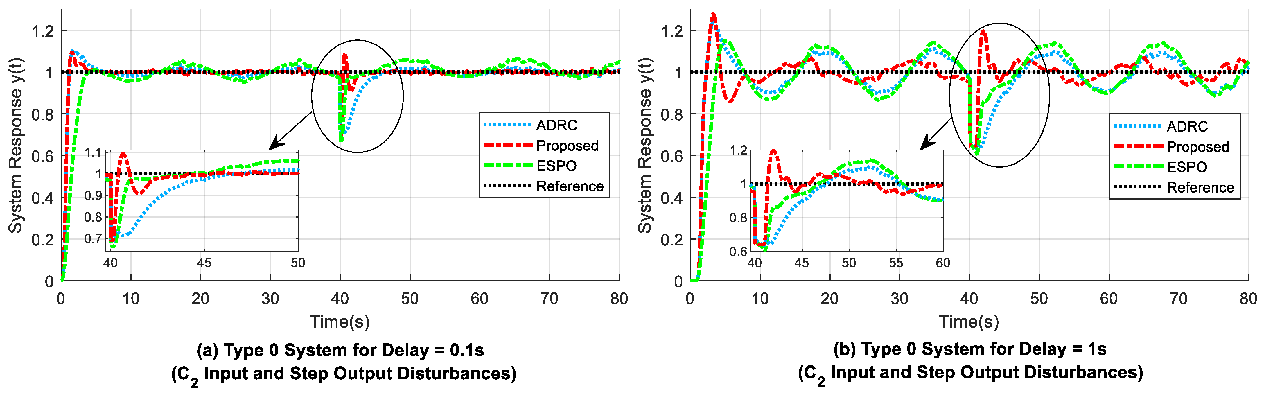
4.1. Experiment 1: Second-Order Type 0 System
- 1.
- The values of the maximum drop from reference () due to output disturbance are similar for all methods, but the adjustment time needed to return to reference () is small for the proposed design compared with the delay-based ADRC (refer to Table 3). For the ESPO method, the response curve does not attain zero SSE after output disturbance compensation (refer to Figure 7a,d,e).
- 2.
- As shown in Table 2, in the case of both disturbances present, i.e., input () and step output disturbances, the proposed system gives the smallest ITAE values of 3.4517 (from 0 s to 40 s), 19.0940 (from 40 s to 80 s), and 22.5330 (from 0 s to 80 s), whereas the corresponding ITAE values for ADRC and ESPO are relatively higher.
- 3.
- A comparison of the rise time () values in Table 3 shows that the considered ADRC and the proposed method had similar readings, unlike high rise times such as 3.0323 s and 2.5485 s as seen for the ESPO design. Further, for the proposed method, in Figure 7b,d, the overshoot (OS) at the beginning of the response curve due to the time delay present is reduced by about 1% and 3.6% when compared to that of the delay-based ADRC.
- 4.
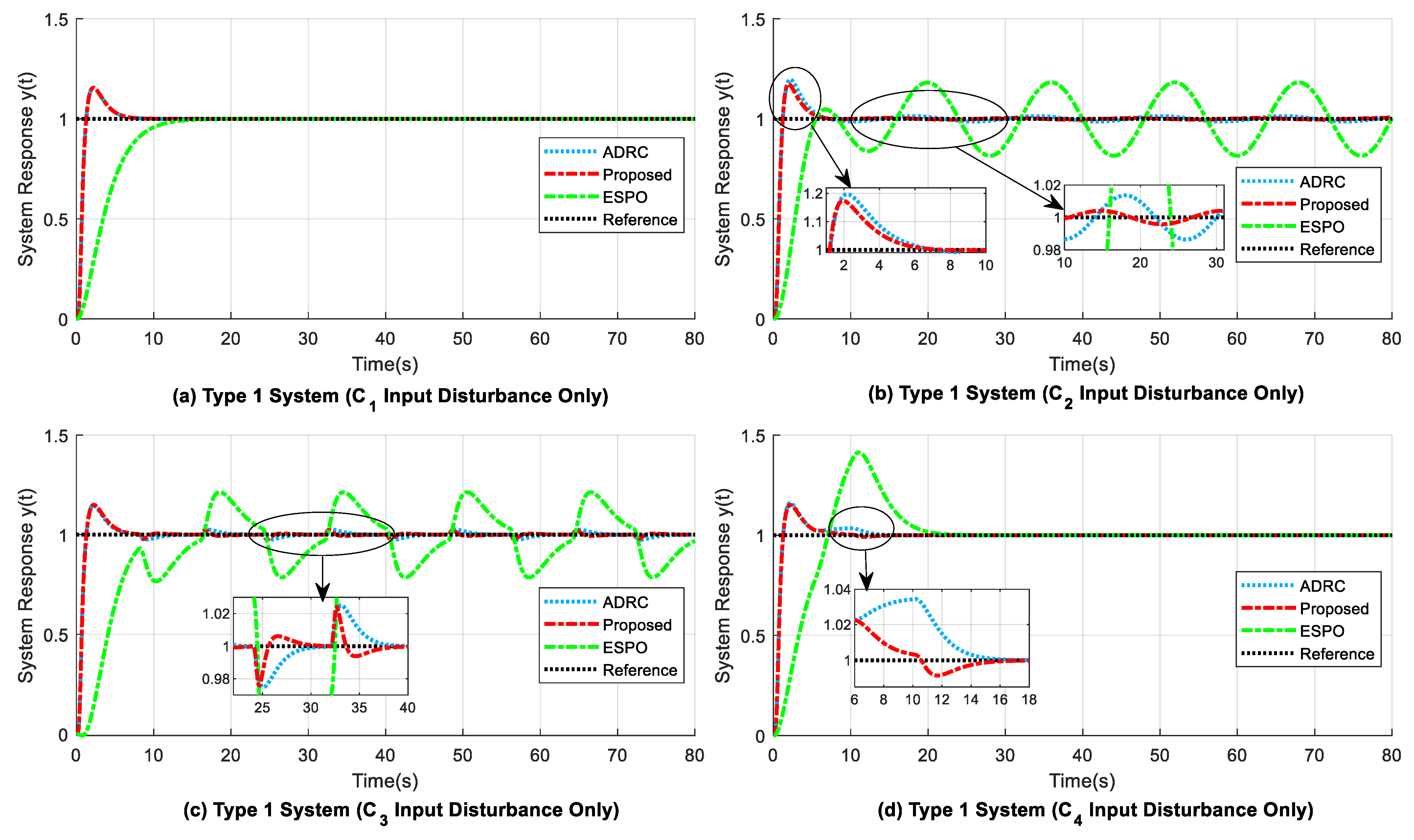
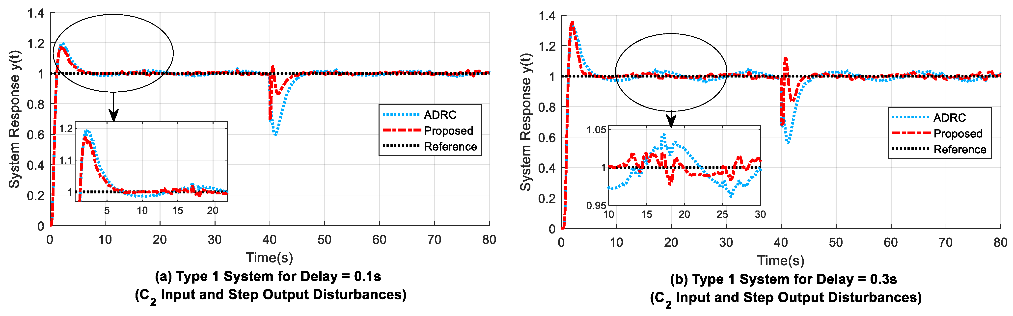
4.2. Experiment 2: Second-Order Type 1 System
- 1.
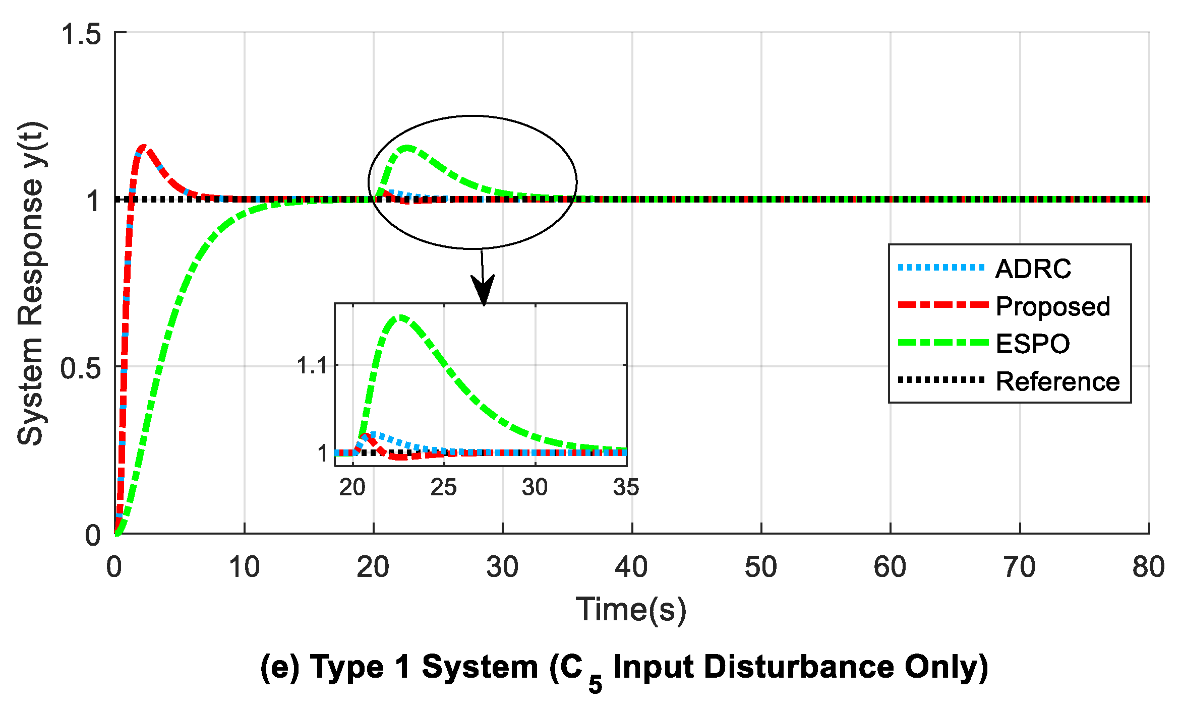
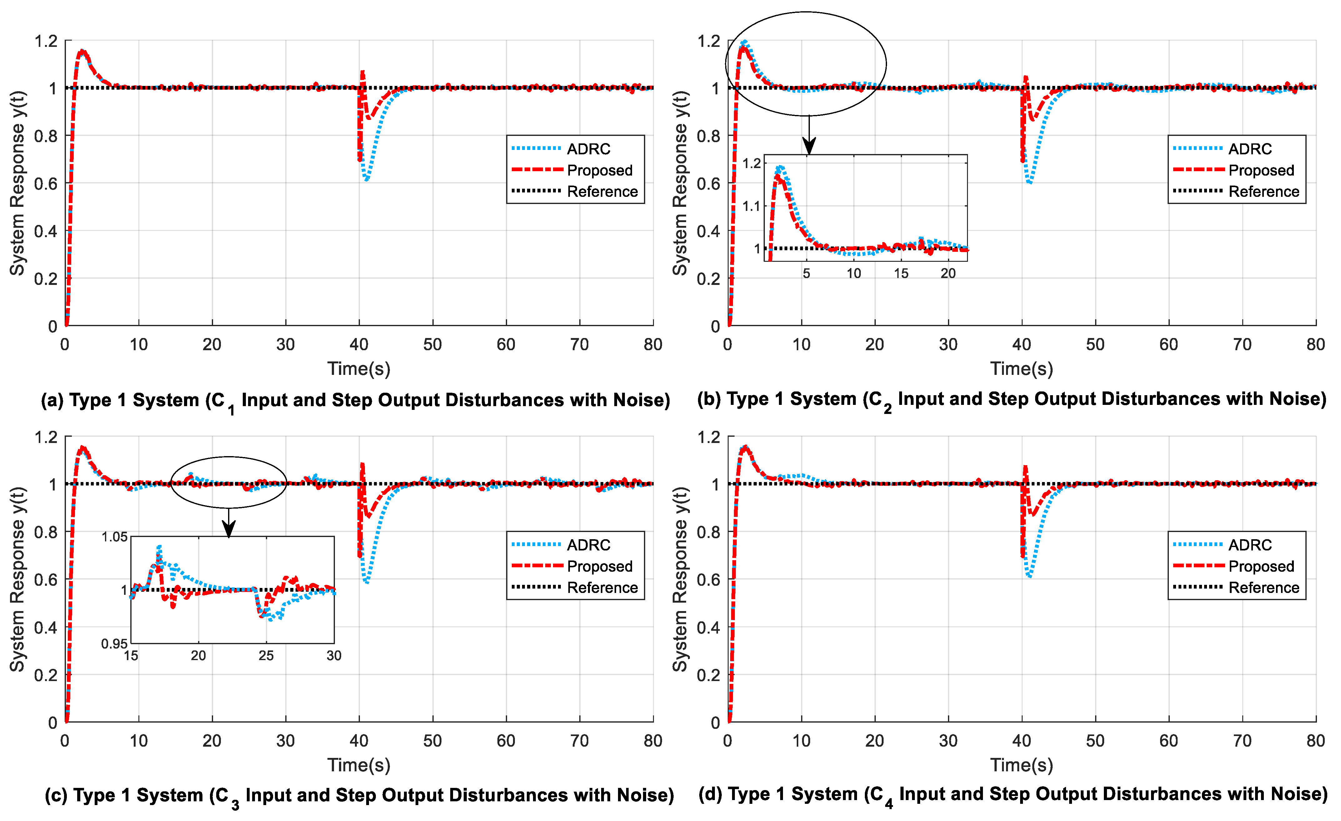
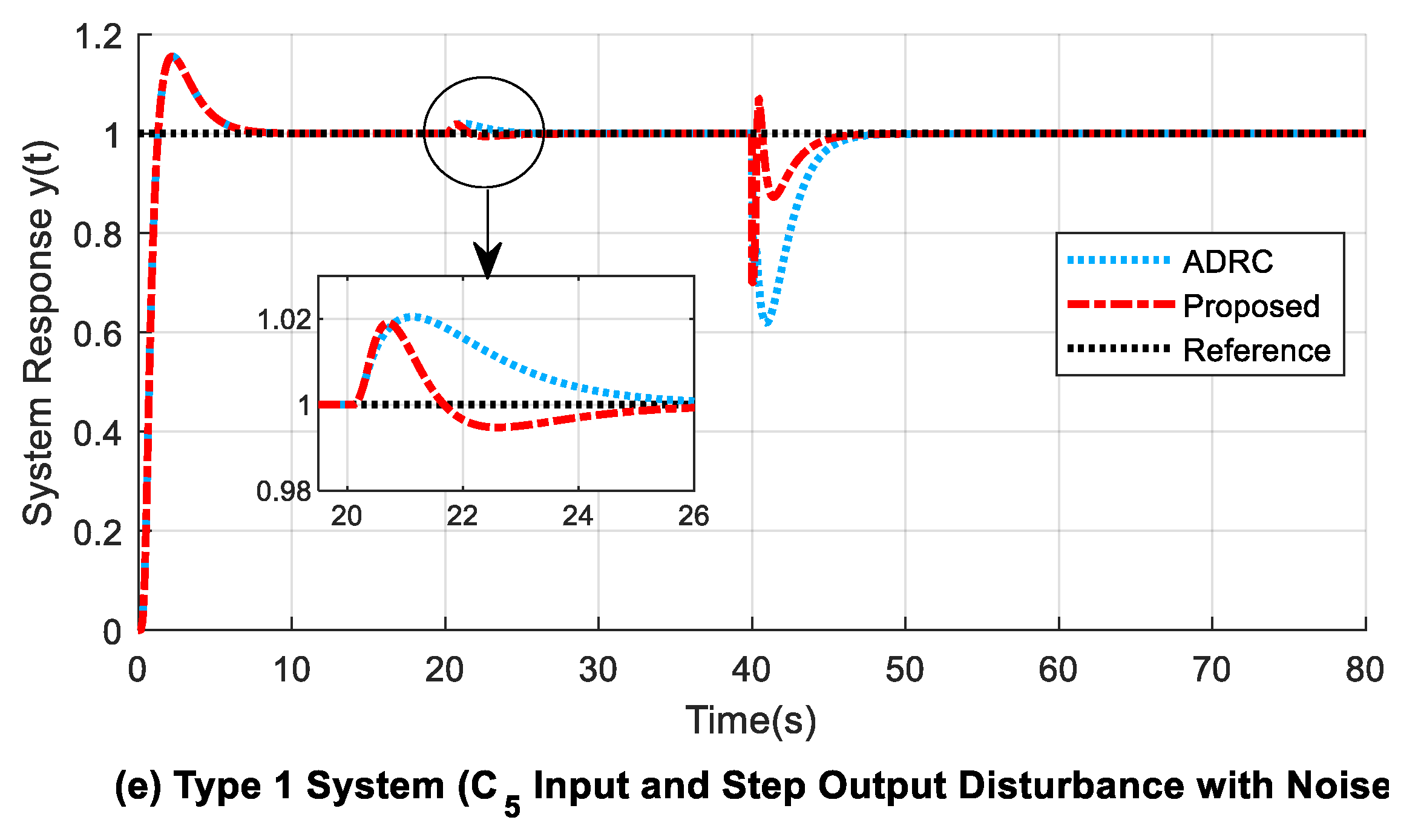
- The maximum drop from reference due to output disturbance () is slightly small for the proposed design when compared with that of the modified ADRC. However, the adjustment time needed to return to reference () is similar for both the former and latter methods. The ESPO method is found to be unstable due to the application of step output disturbance at 40 s (refer to Table 5).
- 2.
- For input () and step output disturbances present, the proposed system gives smaller ITAE values of 4.4819 (from 0 s to 40 s), 24.3140 (from 40 s to 80 s), and 28.7830 (from 0 s to 80 s). The corresponding ITAE values for ADRC are relatively higher, and the ESPO shows unstable behaviour due to step output disturbance.
- 3.
- For the proposed method, in Figure 8b and Figure 9b, the overshoot (OS) at the beginning of the response curve due to the time delay present is reduced by 2.3% when compared to that of the delay-based ADRC structure. Further, at 40 s when step output disturbance is applied (refer to Figure 9a–e), the amplitude of the output disturbance undershoot is reduced by around 25% to 27% in the proposed design, as compared to that of the time-delay-based ADRC structure.
- 4.
- A comparison of the rise times in Table 5 shows that the proposed and modified ADRC methods have similar small rise times (), in contrast to the high rise time for the ESPO method. This indicates that the proposed method shows acceptable behaviour by not making the system slower or unstable, unlike the ESPO design.
- 5.
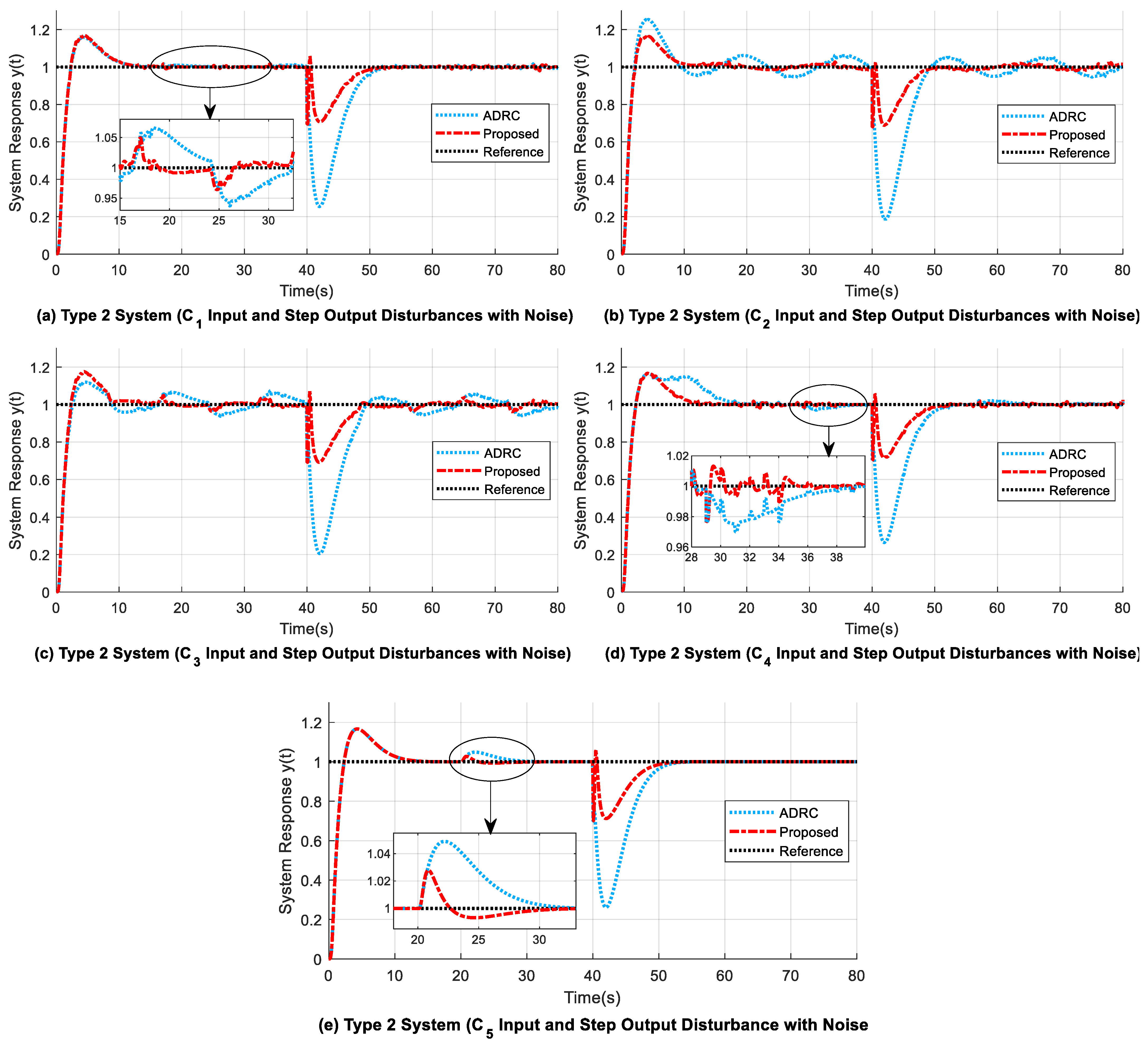
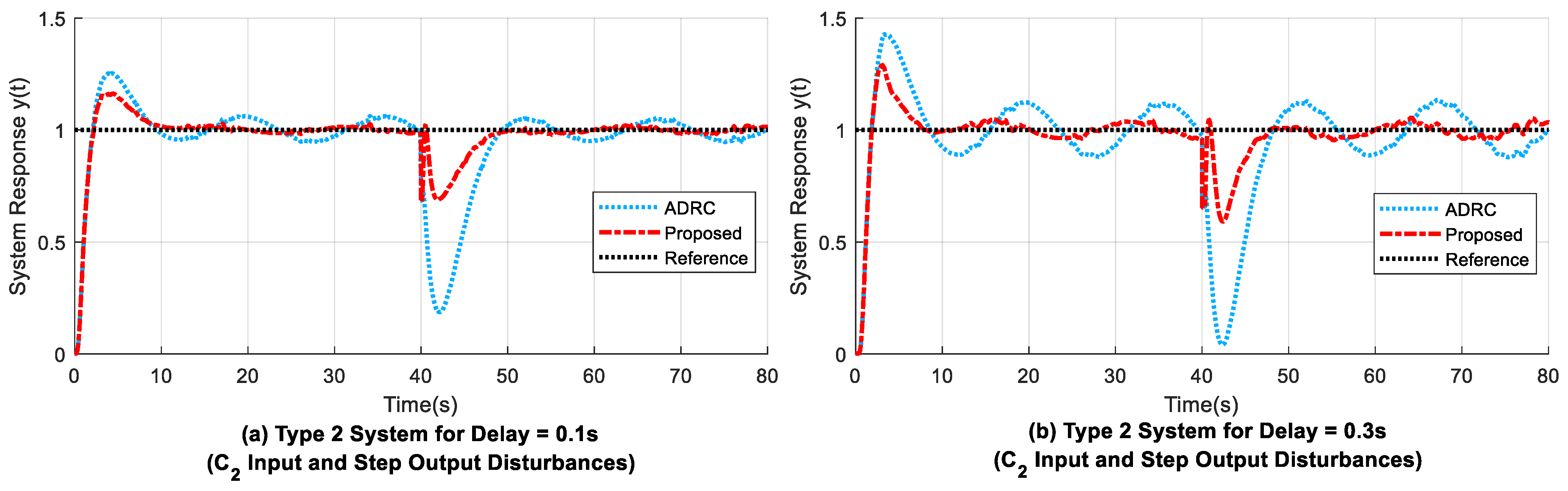
4.3. Experiment 3: Second-Order Type 2 System
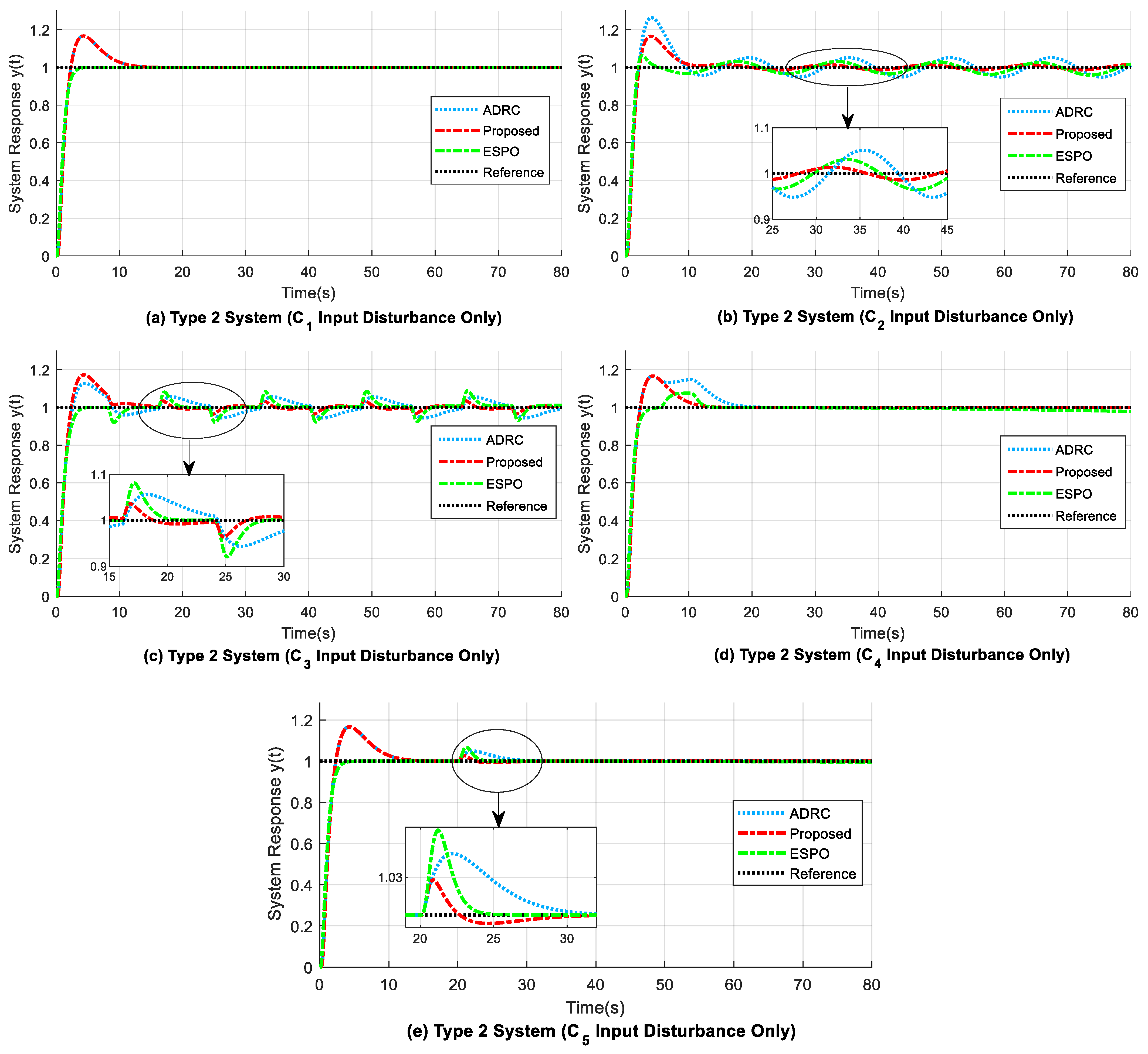
- 1.
- The overshoot (OS) at the start of the response due to time delay is decreased by 9.1% for the proposed structure when compared to that of the modified ADRC (refer to Figure 10b and Figure 11b). In addition, there is a decrease in the time width of the startup overshoot by 67.607% in the proposed design.
- 2.
- As shown in Table 7, the maximum drop from reference due to output disturbance () is less for the proposed design when compared with that of the modified ADRC. Thus, is greatly reduced by around 59% to 61% in the proposed design, as compared to that of the modified ADRC structure (refer to Figure 11a–e). However, the adjustment time needed to return to reference () is similar for both the former and latter methods, whereas the response of the ESPO design becomes unstable when step output disturbance is applied at 40 s (refer to Table 7).
- 3.
- Table 6 shows that the ITAE values for the proposed design are comparatively smaller value than those of the modified ADRC. For example, for input and step output disturbances present, the proposed system has ITAE values of 11.6360 (from 0 s to 40 s), 76.9720 (from 40 s to 80 s), and 88.5950 (from 0 s to 80 s), whereas the corresponding ITAE values for ADRC are relatively higher, and the ESPO shows unstable behaviour due to the step output disturbance applied.
- 4.
- A comparison of the rise time () values in Table 7 shows that the modified ADRC and proposed methods have approximately similar readings, unlike the slightly higher rise times such as 2.110 s seen for the ESPO design.
- 5.
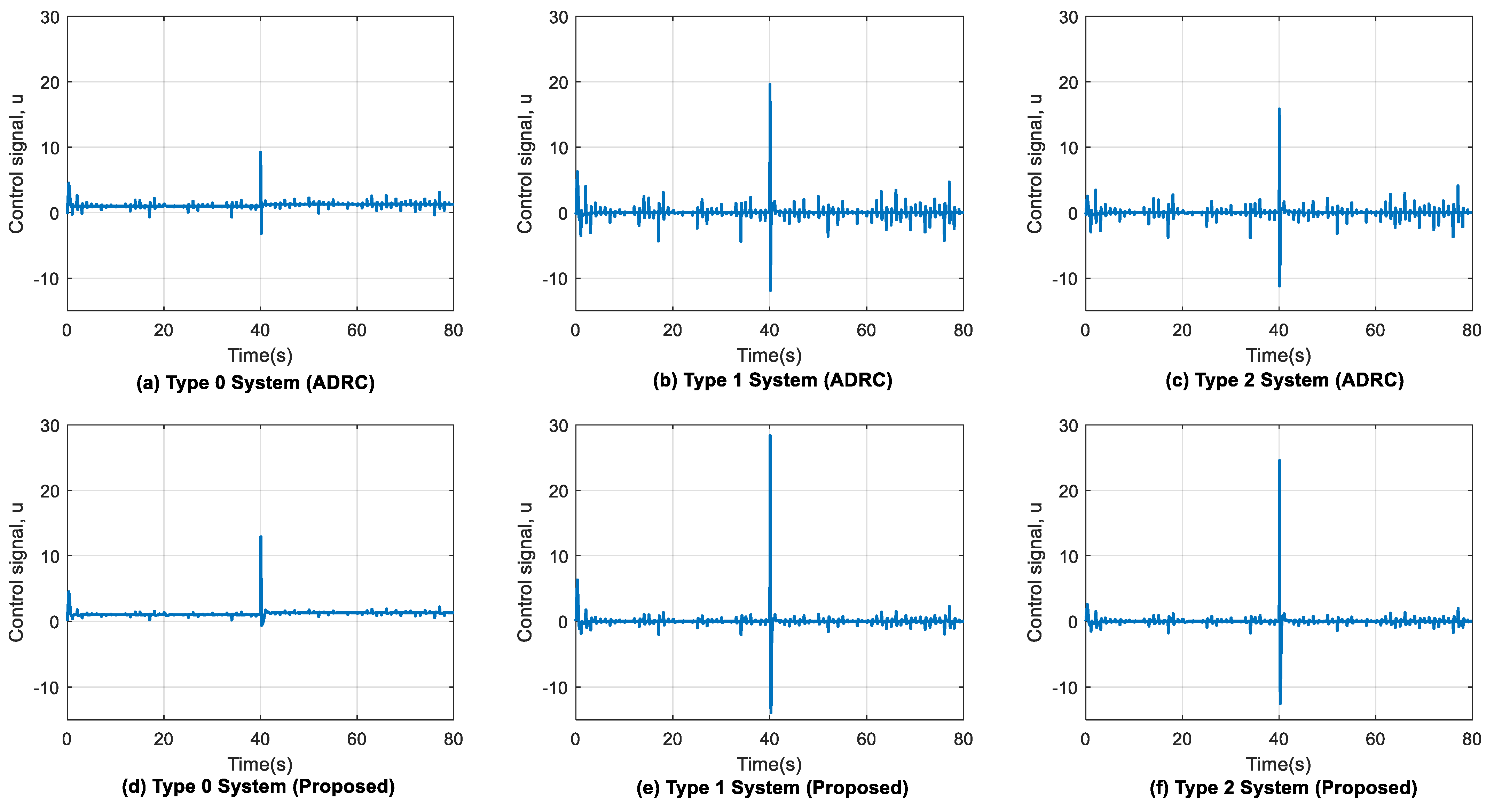
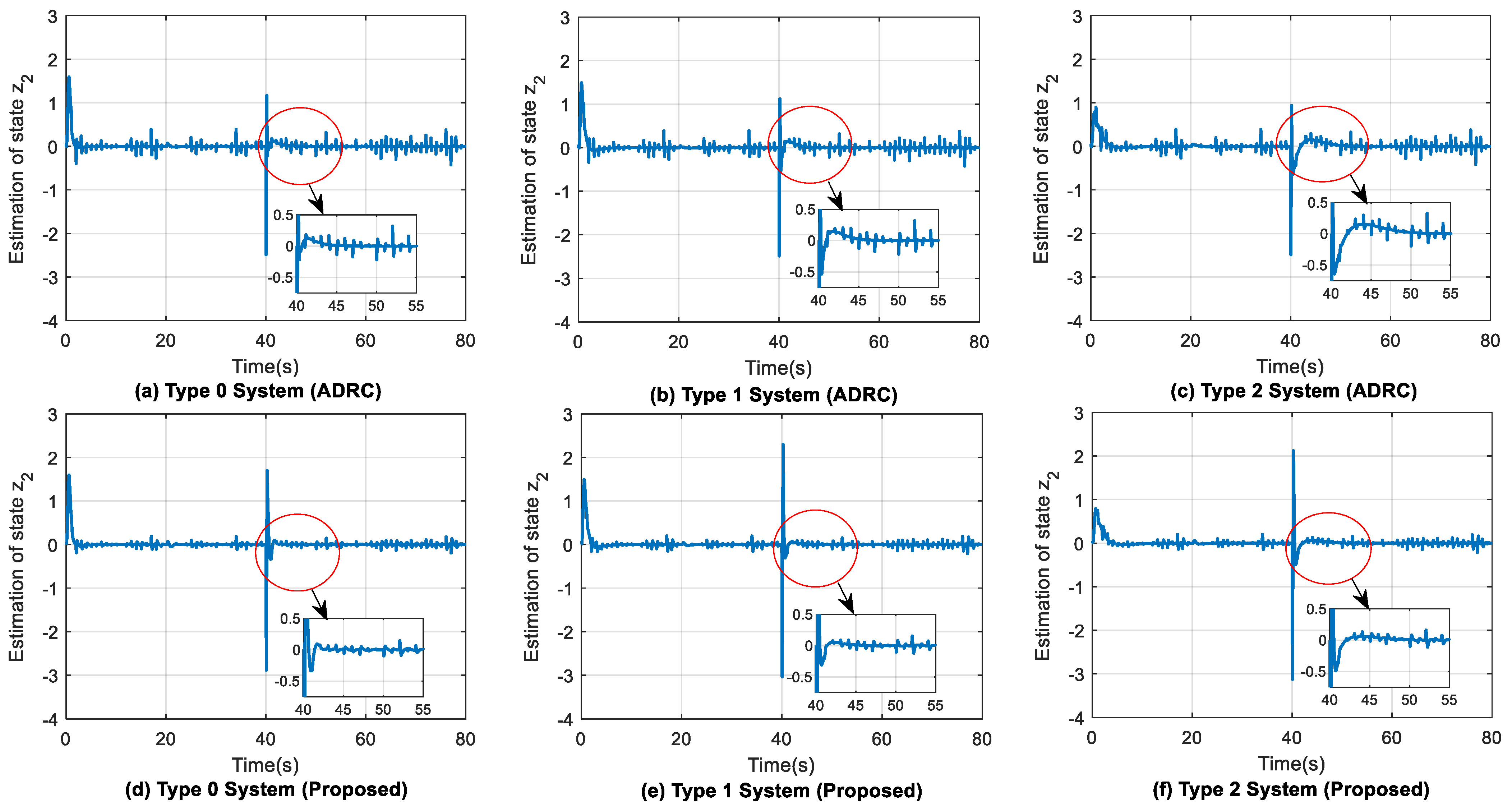
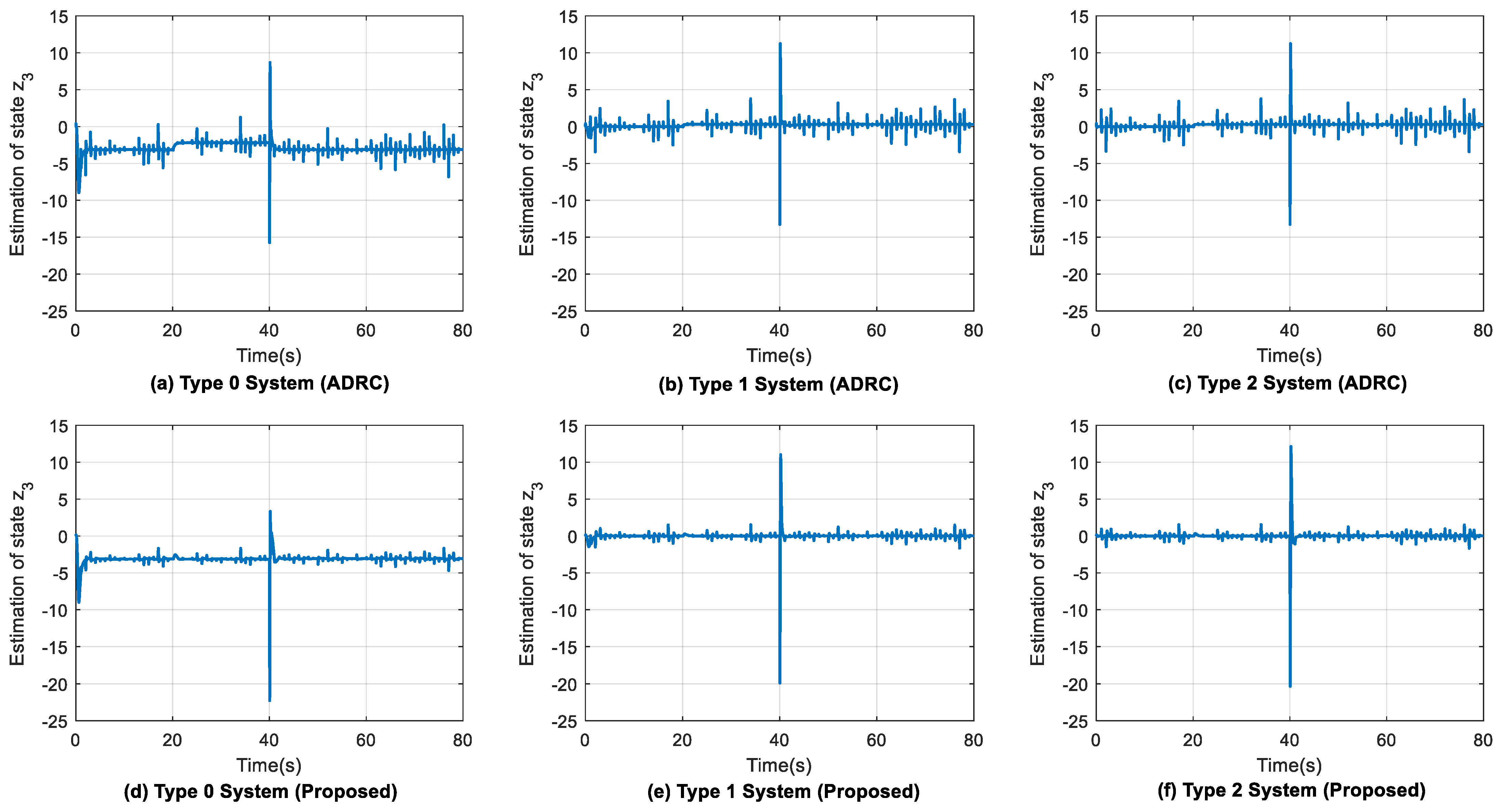
4.4. Effect of Control Signal and ESO States ( and )
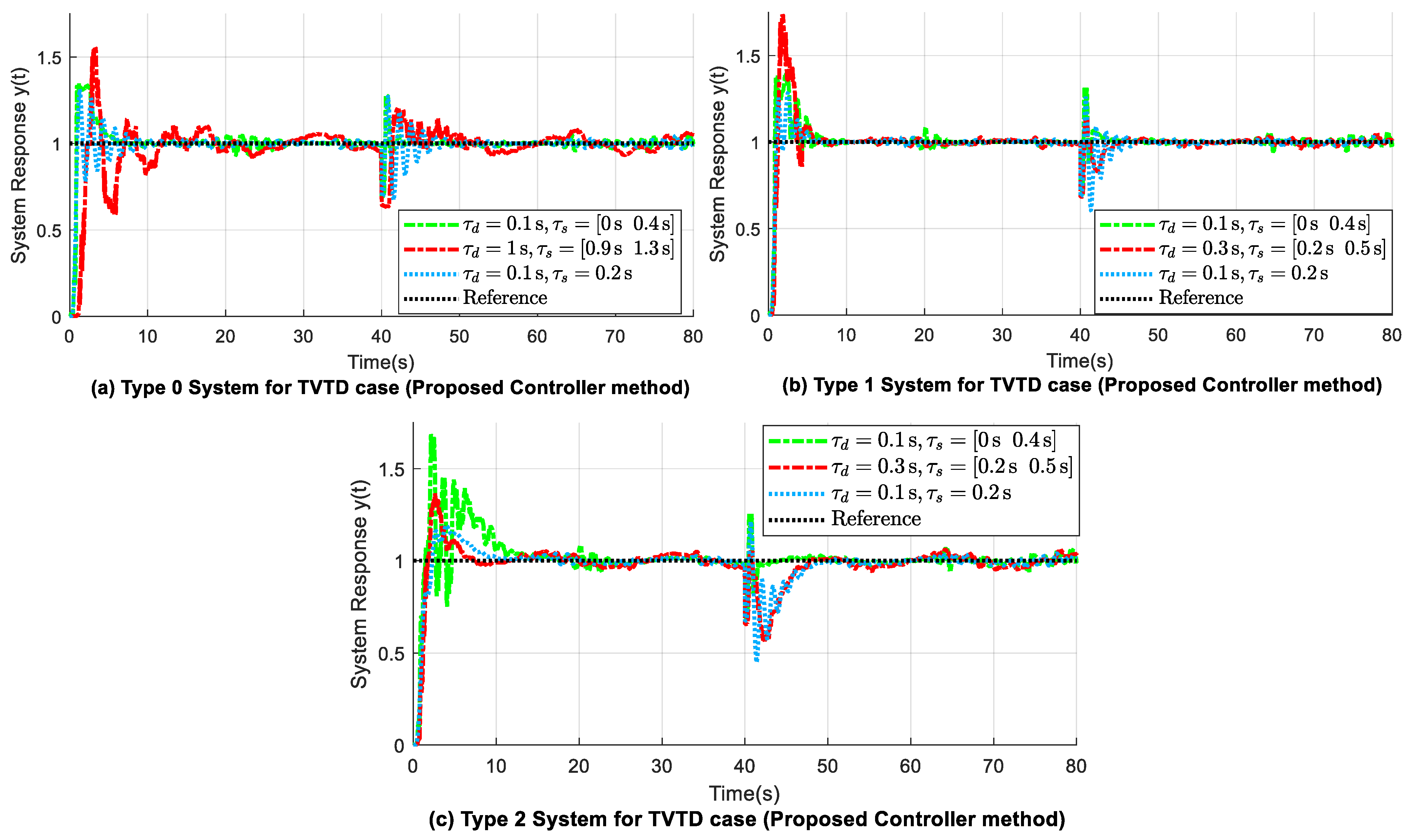
4.5. Effect of Change in Time Delay
5. Discussion
5.1. Disturbance Compensation with Noise and Time Delay
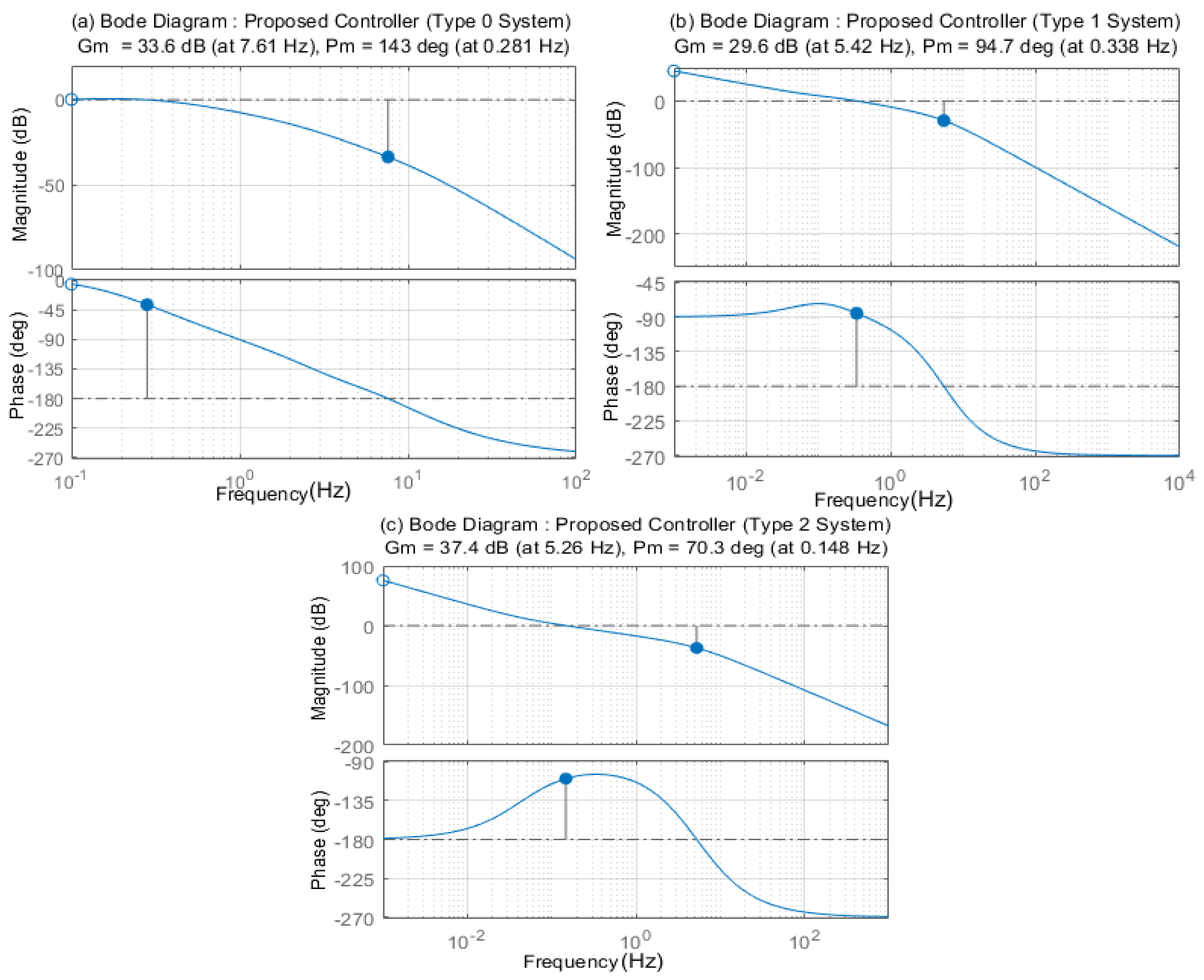
5.2. Rise Time and Bandwidth
5.3. Stability Analysis
5.4. Performance Criteria Analysis
6. Conclusions and Future Recommendations
Author Contributions
Funding
Institutional Review Board Statement
Informed Consent Statement
Data Availability Statement
Conflicts of Interest
References
- Hokayem, P.F.; Spong, M.W. Bilateral teleoperation: An historical survey. Automatica 2006, 42, 2035–2057. [Google Scholar] [CrossRef]
- Richard, J.-P. Time-delay systems: An overview of some recent advances and open problems. Automatica 2003, 39, 1667–1694. [Google Scholar] [CrossRef]
- Shahbazi, M.; Atashzar, S.F.; Patel, R. A Systematic Review of Multilateral Teleoperation Systems. IEEE Trans. Haptics 2018, 11, 338–356. [Google Scholar] [CrossRef] [PubMed]
- Nahri, S.N.F.; Du, S.; Van Wyk, B.J. A Review on Haptic Bilateral Teleoperation Systems. J. Intell. Robot. Syst. 2022, 104, 13. [Google Scholar] [CrossRef]
- Han, J. A class of extended state observers for uncertain systems. Control Decis. 1995, 10, 85–88. [Google Scholar]
- Han, J.Q. Auto Disturbance Rejection Controller and It’s Applications. Control Decis. 1998, 13, 19–23. [Google Scholar] [CrossRef]
- Han, J. From PID to Active Disturbance Rejection Control. IEEE Trans. Ind. Electron. 2009, 56, 900–906. [Google Scholar] [CrossRef]
- Gao, Z. On the centrality of disturbance rejection in automatic control. ISA Trans. 2014, 53, 850–857. [Google Scholar] [CrossRef] [Green Version]
- Feng, H.; Guo, B.-Z. Active disturbance rejection control: Old and new results. Annu. Rev. Control 2017, 44, 238–248. [Google Scholar] [CrossRef]
- Chu, Z.; Wu, C.; Sepehri, N. Active disturbance rejection control applied to high-order systems with parametric uncertainties. Int. J. Control Autom. Syst. 2019, 17, 1483–1493. [Google Scholar] [CrossRef]
- He, T.; Wu, Z.; Li, D.; Wang, J. A tuning method of active disturbance rejection control for a class of high-order processes. IEEE Trans. Ind. Electron. 2019, 67, 3191–3201. [Google Scholar] [CrossRef]
- Wu, Z.; Shi, G.; Li, D.; Liu, Y.; Chen, Y. Active disturbance rejection control design for high-order integral systems. ISA Trans. 2022, 125, 560–570. [Google Scholar] [CrossRef]
- Wu, Z.; Gao, Z.; Li, D.; Chen, Y.; Liu, Y. On transitioning from PID to ADRC in thermal power plants. Control Theory Technol. 2021, 19, 3–18. [Google Scholar] [CrossRef]
- Fareh, R.; Khadraoui, S.; Abdallah, M.Y.; Baziyad, M.; Bettayeb, M. Active disturbance rejection control for robotic systems: A review. Mechatronics 2021, 80, 102671. [Google Scholar] [CrossRef]
- Nahri, S.N.F.; Du, S.; van Wyk, B.J. Active Disturbance Rejection Control Design for a Haptic Machine Interface Platform. Adv. Sci. Technol. Eng. Syst. J. 2021, 6, 898–911. [Google Scholar] [CrossRef]
- Wang, F.; Liu, P.; Xie, M.; Jing, F.; Liu, B.; Cao, Y.; Ma, C. Robust Reduced-Order Active Disturbance Rejection Control Method: A Case Study on Speed Control of a One-Dimensional Gimbal. Machines 2022, 10, 592. [Google Scholar] [CrossRef]
- Sun, A.; Songmao, P.; He, Z.; Xiao, K.; Sun, P.; Wang, P.; Wei, X. Application of model free active disturbance rejection controller in nuclear reactor power control. Prog. Nucl. Energy 2021, 140, 103907. [Google Scholar] [CrossRef]
- Niculescu, S.-I. Delay Effects on Stability: A Robust Control Approach; Springer Science & Business Media: Berlin/Heidelberg, Germany, 2001; Volume 269. [Google Scholar]
- Wang, L.; Li, Q.; Tong, C.; Yin, Y. Overview of active disturbance rejection control for systems with time-delay. Control Theory Appl. 2013, 30, 1521–1533. [Google Scholar] [CrossRef]
- Chen, S.; Xue, W.; Zhong, S.; Huang, Y. On comparison of modified ADRCs for nonlinear uncertain systems with time delay. Sci. China Inf. Sci. 2018, 61, 70223. [Google Scholar] [CrossRef] [Green Version]
- Xia, Y.; Liu, G.P.; Shi, P.; Han, J.; Rees, D. Active disturbance rejection control for uncertain multivariable systems with time-delay. IET Control Theory Appl. 2007, 1, 75–81. [Google Scholar] [CrossRef]
- Pawar, S.N.; Chile, R.H.; Patre, B.M. Predictive extended state observer-based robust control for uncertain linear systems with experimental validation. Trans. Inst. Meas. Control 2021, 43, 2615–2627. [Google Scholar] [CrossRef]
- Chen, G.; Liu, D.; Mu, Y.; Xu, J.; Cheng, Y. A Novel Smith Predictive Linear Active Disturbance Rejection Control Strategy for the First-Order Time-Delay Inertial System. Math. Probl. Eng. 2021, 2021, 5560123. [Google Scholar] [CrossRef]
- Li, P.; Wang, L.; Zhu, G.; Zhang, M. Predictive active disturbance rejection control for servo systems with communication delays via sliding mode approach. IEEE Trans. Ind. Electron. 2020, 68, 12679–12688. [Google Scholar] [CrossRef]
- Artheec Kumar, V.; Cao, Z.; Man, Z.; Chuei, R.; Bombuwela, D. Predictive extended state observer-based repetitive controller for uncertain systems with input delay. Automatika 2022, 63, 122–131. [Google Scholar] [CrossRef]
- Wang, C.; Zuo, Z.; Qi, Z.; Ding, Z. Predictor-based extended-state-observer design for consensus of MASs with delays and disturbances. IEEE Trans. Cybern. 2018, 49, 1259–1269. [Google Scholar] [CrossRef] [PubMed]
- Castillo, A.; Santos, T.L.; Garcia, P.; Normey-Rico, J.E. Predictive ESO-based control with guaranteed stability for uncertain MIMO constrained systems. ISA Trans. 2021, 112, 161–167. [Google Scholar] [CrossRef] [PubMed]
- Zheng, Q.; Gao, Z. Predictive active disturbance rejection control for processes with time delay. ISA Trans. 2014, 53, 873–881. [Google Scholar] [CrossRef] [PubMed]
- Xue, W.; Liu, P.; Chen, S.; Huang, Y. On Extended State Predictor Observer Based Active Disturbance Rejection Control for Uncertain Systems with Sensor Delay. In Proceedings of the 2016 16th International Conference on Control, Automation and Systems (ICCAS), Gyeongju, Korea, 16–19 October 2016; pp. 1267–1271. [Google Scholar]
- Tan, W.; Fu, C. Analysis of Active Disturbance Rejection Control for Processes with Time Delay. In Proceedings of the 2015 American Control Conference (ACC), Chicago, IL, USA, 1–3 July 2015; pp. 3962–3967. [Google Scholar]
- Zhang, B.; Tan, W.; Li, J. Tuning of Smith predictor based generalized ADRC for time-delayed processes via IMC. ISA Trans. 2020, 99, 159–166. [Google Scholar] [CrossRef]
- Cheng, Y.; Chen, Z.; Sun, M.; Sun, Q. Active disturbance rejection generalized predictive control for a high purity distillation column process with time delay. Can. J. Chem. Eng. 2019, 97, 2941–2951. [Google Scholar] [CrossRef]
- Fu, C.; Tan, W. Linear active disturbance rejection control for processes with time delays: IMC interpretation. IEEE Access 2020, 8, 16606–16617. [Google Scholar] [CrossRef]
- Chen, S.; Xue, W.; Huang, Y.; Liu, P. On Comparison between Smith Predictor and Predictor Observer Based Adrcs for Nonlinear Uncertain Systems with Output Delay. In Proceedings of the 2017 American Control Conference (ACC), Seattle, WA, USA, 24–26 May 2017; pp. 5083–5088. [Google Scholar]
- Zhao, S.; Gao, Z. Modified active disturbance rejection control for time-delay systems. ISA Trans. 2014, 53, 882–888. [Google Scholar] [CrossRef]
- Wang, S.; Sun, G.; Liu, S. Active disturbance rejection sliding mode control for time-delay systems. J. Syst. Simul. 2019, 31, 102. [Google Scholar]
- Ran, M.; Wang, Q.; Dong, C.; Xie, L. Active disturbance rejection control for uncertain time-delay nonlinear systems. Automatica 2020, 112, 108692. [Google Scholar] [CrossRef]
- Wang, X.; Zhou, Y.; Zhao, Z.; Wei, W.; Li, W. Time-delay system control based on an integration of active disturbance rejection and modified twice optimal control. IEEE Access 2019, 7, 130734–130744. [Google Scholar] [CrossRef]
- Zheng, Q.; Gao, L.Q.; Gao, Z. On Validation of Extended State Observer Through Analysis and Experimentation. J. Dyn. Syst. Meas. Control 2012, 134, 024505. [Google Scholar] [CrossRef]
- YV Wen-bin, Y.D. Modeling and Simulation of an Active Disturbance Rejection Controller Based on Matlab/Simulink. Int. J. Res. Eng. Sci. 2015, 3, 62–69. [Google Scholar]
- Han, J.-q. Auto disturbances rejection control technique. Front. Sci. 2007, 1, 24–31. [Google Scholar]
- Jiang, P.; Hao, J.-Y.; Zong, X.-P.; Wang, P.-G. Modeling and Simulation of Active-Disturbance-Rejection Controller with Simulink. In Proceedings of the 2010 International Conference on Machine Learning and Cybernetics, Qingdao, China, 11–14 July 2010; pp. 927–931. [Google Scholar]
- Gao, Z. Scaling and Bandwidth-Parameterization Based Controller Tuning. In Proceedings of the American Control Conference, Denver, CO, USA, 4–6 June 2003; pp. 4989–4996. [Google Scholar]
- Yoo, D.; Yau, S.-T.; Gao, Z. Optimal fast tracking observer bandwidth of the linear extended state observer. Int. J. Control 2007, 80, 102–111. [Google Scholar] [CrossRef]
- Zhang, X.; Zhang, X.; Xue, W.; Xin, B. An overview on recent progress of extended state observers for uncertain systems: Methods, theory, and applications. Adv. Control Appl. Eng. Ind. Syst. 2021, 3, e89. [Google Scholar] [CrossRef]
- Martins, F.G. Tuning PID controllers using the ITAE criterion. Int. J. Eng. Educ. 2005, 21, 867. [Google Scholar]
- Saraswat, M.; Sharma, A. Genetic Algorithm for optimization using MATLAB. Int. J. Adv. Res. Comput. Sci. 2013, 4, 155–159. [Google Scholar]
- Rasolomampionona, D.; Klos, M.; Cirit, C.; Montegiglio, P.; De Tuglie, E.E. A New Method for Optimization of Load Frequency Control Parameters in Multi-Area Power Systems Using Genetic Algorithms. In Proceedings of the 2022 IEEE International Conference on Environment and Electrical Engineering and 2022 IEEE Industrial and Commercial Power Systems Europe (EEEIC/I&CPS Europe), Prague, Czech Republic, 28 June–1 July 2022; pp. 1–9. [Google Scholar]
- Nahri, S.N.F.; Du, S.; Van Wyk, B. Haptic System Interface Design and Modelling for Bilateral Teleoperation Systems. In Proceedings of the 2020 International SAUPEC/RobMech/PRASA Conference, Cape Town, South Africa, 29–31 January 2020; pp. 1–6. [Google Scholar]


| Delay-Based ADRC | ||||||
|---|---|---|---|---|---|---|
| Type 0 System | 0.7645 | 1.0831 | 56.0350 | 0.3097 | 3.1303 | 1.0314 |
| Type 1 System | 1.0710 | 0.9340 | 41.5480 | 1.0000 | 1.0000 | 1.0000 |
| Type 2 System | 0.8990 | 2.0216 | 62.9887 | 1.0000 | 1.0000 | 1.0000 |
| Input Disturbance Number | Method | With Input Disturbance () * | With Input Disturbance () *, Output Disturbance, and Noise | ||||
|---|---|---|---|---|---|---|---|
| ITAE (0–40 s) | ITAE (40–80 s) | ITAE (0–80 s) | ITAE (0–40 s) | ITAE (40–80 s) | ITAE (0–80 s) | ||
| = 1 | ADRC | 0.6676 | 0.0009 | 1.0607 | 1.6124 | 31.1490 | 32.7500 |
| Proposed | 0.6676 | 0.0009 | 0.6685 | 2.5574 | 17.4630 | 20.0080 | |
| ESPO | 2.3805 | 0 | 2.3805 | 4.3932 | 50.4860 | 54.8670 | |
| = 2 | ADRC | 9.6014 | 27.387 | 36.988 | 9.7792 | 53.7620 | 63.5280 |
| Proposed | 2.25885 | 5.1091 | 7.3678 | 3.4517 | 19.0940 | 22.5330 | |
| ESPO | 21.6490 | 62.9280 | 84.5760 | 21.2200 | 72.2790 | 93.4850 | |
| = 3 | ADRC | 8.2367 | 24.8410 | 33.0780 | 8.6993 | 53.2740 | 61.9610 |
| Proposed | 3.8284 | 10.7540 | 14.5830 | 4.6495 | 21.6770 | 26.3140 | |
| ESPO | 18.3780 | 54.2800 | 72.6580 | 18.8440 | 77.7070 | 96.5380 | |
| = 4 | ADRC | 3.0302 | 0.0003 | 3.0304 | 3.9263 | 30.2750 | 34.1890 |
| Proposed | 1.0168 | 0.0009 | 1.0177 | 2.9576 | 18.5780 | 21.5230 | |
| ESPO | 6.6778 | 0 | 6.6778 | 8.6929 | 52.2850 | 60.9650 | |
| = 5 | ADRC | 2.2397 | 0.0006 | 2.2403 | 3.1505 | 31.1490 | 34.2880 |
| Proposed | 1.3506 | 0.0009 | 1.3515 | 3.1726 | 17.4630 | 20.6230 | |
| ESPO | 5.7809 | 4.7184 × 10⁻⁶ | 5.7809 | 7.7430 | 50.4860 | 58.2160 | |
| Input Disturbance Number | Method | With Input Disturbance ( ) * | With Input Disturbance () *, Output Disturbance, and Noise | |||||
|---|---|---|---|---|---|---|---|---|
| OS (%) | OS (%) | |||||||
| = 1 | ADRC | 6.0700 | 0.6478 | 0 | 6.0700 | 0.6298 | 0.2721 | 8.0300 |
| Proposed | 6.0700 | 0.6478 | 0 | 5.8200 | 0.6308 | 0.3051 | 5.6500 | |
| ESPO | 0 | 2.8782 | 0 | 0.7200 | 3.0323 | 0.3051 | Non-zero finite SSE | |
| = 2 | ADRC | 10.7500 | 0.6459 | 0.0182 | 10.7300 | 0.6299 | 0.3190 | 7.0600 |
| Proposed | 9.8400 | 0.6121 | 0.0031 | 9.3800 | 0.6002 | 0.3085 | 5.3800 | |
| ESPO | 1.8300 | 2.4102 | 0.0418 | 1.8400 | 2.4449 | 0.3374 | 4.2400 | |
| = 3 | ADRC | 7.5100 | 0.5966 | 0.0387 | 7.5200 | 0.5943 | 0.3088 | 8.1700 |
| Proposed | 5.4900 | 0.5982 | 0.0358 | 5.6300 | 0.5960 | 0.3052 | 5.5500 | |
| ESPO | 0 | 2.3637 | 0.0946 | 0.4800 | 2.3880 | 0.3052 | 3.2300 | |
| = 4 | ADRC | 8.9500 | 0.6075 | 0.0030 | 8.9000 | 0.6019 | 0.2678 | 9.0200 |
| Proposed | 8.9500 | 0.6075 | 0.0030 | 5.2100 | 0.6060 | 0.3056 | 5.7200 | |
| ESPO | 1.0270 | 2.5169 | 0.1030 | 10.4200 | 2.5485 | 0.3056 | Non-zero finite SSE | |
| = 5 | ADRC | 6.0700 | 0.6478 | 0.0320 | 6.0700 | 0.6298 | 0.3051 | 8.0100 |
| Proposed | 6.0700 | 0.6478 | 0.0290 | 5.8200 | 0.6308 | 0.3057 | 5.5000 | |
| ESPO | 7.3900 | 2.8782 | 0.0740 | 0.7200 | 3.0323 | 0.3000 | Non-zero finite SSE | |
| Input Disturbance Number | Method | With Input Disturbance () * | With Input Disturbance () *, Output Disturbance, and Noise | ||||
|---|---|---|---|---|---|---|---|
| ITAE (0–40 s) | ITAE (40–80 s) | ITAE (0–80 s) | ITAE (0–40 s) | ITAE (40–80 s) | ITAE (0–80 s) | ||
| = 1 | ADRC | 1.5766 | 9.8378 × 10⁻¹¹ | 1.5766 | 2.8122 | 47.5200 | 50.3200 |
| Proposed | 1.5766 | 9.8378 × 10⁻¹¹ | 1.5766 | 3.3515 | 22.6150 | 25.9540 | |
| ESPO | 12.4050 | 4.0049 × 10⁻⁶ | 12.4050 | Unstable | Unstable | Unstable | |
| = 2 | ADRC | 8.2185 | 20.4950 | 28.7130 | 8.9441 | 62.972 | 71.903 |
| Proposed | 3.4850 | 6.3879 | 9.8729 | 4.4819 | 24.3140 | 28.7830 | |
| ESPO | 93.1820 | 280.2800 | 373.4600 | Unstable | Unstable | Unstable | |
| = 3 | ADRC | 7.0513 | 18.5120 | 25.5630 | 7.8534 | 63.0580 | 70.8990 |
| Proposed | 4.6276 | 10.1540 | 14.7820 | 5.3395 | 28.0510 | 33.3780 | |
| ESPO | 102.6800 | 284.4000 | 387.0800 | Unstable | Unstable | Unstable | |
| = 4 | ADRC | 3.2785 | 1.1437 × 10⁻¹⁰ | 3.2785 | 4.4735 | 47.4000 | 51.8610 |
| Proposed | 2.0698 | 1.3578 × 10⁻¹⁰ | 2.0698 | 3.7814 | 22.9790 | 26.7480 | |
| ESPO | 38.9340 | 0.0006 | 38.9340 | Unstable | Unstable | Unstable | |
| = 5 | ADRC | 2.7463 | 2.2000 × 10⁻⁷ | 2.7463 | 3.9124 | 47.5200 | 51.4200 |
| Proposed | 2.2268 | 2.0090 × 10⁻⁷ | 2.2268 | 3.9120 | 22.6150 | 26.5150 | |
| ESPO | 33.1020 | 0.0229 | 33.1250 | Unstable | Unstable | Unstable | |
| Input Disturbance Number | Method | With Input Disturbance () * | With Input Disturbance () *, Output Disturbance, and Noise | |||||
|---|---|---|---|---|---|---|---|---|
| OS (%) | OS (%) | |||||||
| = 1 | ADRC | 15.5500 | 0.6940 | 0 | 15.5800 | 0.6750 | 0.3903 | 9.0100 |
| Proposed | 15.5500 | 0.6940 | 0 | 16.1500 | 0.6771 | 0.3054 | 9.0100 | |
| ESPO | 0 | 6.7158 | 0 | Unstable | Unstable | Unstable | Unstable | |
| = 2 | ADRC | 19.7100 | 0.6767 | 0.0140 | 19.4800 | 0.6596 | 0.4049 | 7.0000 |
| Proposed | 17.3800 | 0.6534 | 0.0041 | 17.1600 | 0.6399 | 0.3095 | 7.0000 | |
| ESPO | 4.7300 | 3.5289 | 0.1847 | Unstable | Unstable | Unstable | Unstable | |
| = 3 | ADRC | 14.6700 | 0.6884 | 0.0250 | 14.8900 | 0.6691 | 0.4173 | 8.0400 |
| Proposed | 15.0200 | 0.6991 | 0.0242 | 16.0800 | 0.6803 | 0.3054 | 8.0400 | |
| ESPO | 0 | 5.1066 | 0.2147 | Unstable | Unstable | Unstable | Unstable | |
| = 4 | ADRC | 16.1500 | 0.6781 | 0.0340 | 16.1200 | 0.6598 | 0.3916 | 8.0000 |
| Proposed | 15.1300 | 0.6789 | 0.0086 | 15.7500 | 0.6622 | 0.3055 | 8.0000 | |
| ESPO | 41.4200 | 5.2571 | 0.4140 | Unstable | Unstable | Unstable | Unstable | |
| = 5 | ADRC | 15.5500 | 0.6940 | 0.0200 | 15.5800 | 0.6750 | 0.3899 | 8.0000 |
| Proposed | 15.5500 | 0.6940 | 0.0190 | 16.1500 | 0.6771 | 0.3055 | 7.3200 | |
| ESPO | 15.3600 | 6.7158 | 0.1540 | Unstable | Unstable | Unstable | Unstable | |
| Input Disturbance Number | Method | With Input Disturbance () * | With Input Disturbance () *, Output Disturbance, and Noise | ||||
|---|---|---|---|---|---|---|---|
| ITAE (0–40 s) | ITAE (40–80 s) | ITAE (0–80 s) | ITAE (0–40 s) | ITAE (40–80 s) | ITAE (0–80 s) | ||
| = 1 | ADRC | 5.6431 | 1.3318 × 10⁻⁶ | 5.6431 | 8.3739 | 167.5400 | 175.9000 |
| Proposed | 5.6431 | 1.3318 × 10⁻⁶ | 5.6431 | 7.4086 | 68.3370 | 75.7330 | |
| ESPO | 0.8550 | 5.0639 × 10⁻¹² | 0.8550 | Unstable | Unstable | Unstable | |
| = 2 | ADRC | 29.9070 | 77.8620 | 107.7700 | 32.2100 | 229.5100 | 261.7100 |
| Proposed | 11.3450 | 21.2620 | 32.6060 | 11.6360 | 76.9720 | 88.5950 | |
| ESPO | 16.5060 | 51.3300 | 67.8250 | Unstable | Unstable | Unstable | |
| = 3 | ADRC | 27.8760 | 78.8290 | 106.7000 | 30.1880 | 230.4000 | 260.5800 |
| Proposed | 12.4240 | 23.7290 | 36.1520 | 12.6680 | 79.5770 | 92.2330 | |
| ESPO | 13.9060 | 48.5680 | 62.4720 | Unstable | Unstable | Unstable | |
| = 4 | ADRC | 14.5970 | 5.9430 × 10⁻⁶ | 14.5970 | 19.7420 | 168.6300 | 188.3600 |
| Proposed | 5.6431 | 1.3318 × 10⁻⁶ | 5.6431 | 8.0527 | 65.4530 | 73.4940 | |
| ESPO | 5.6828 | 29.7870 | 35.4680 | Unstable | Unstable | Unstable | |
| = 5 | ADRC | 11.3930 | 0.0021 | 11.3950 | 13.9520 | 167.5400 | 181.4800 |
| Proposed | 7.2863 | 0.0007 | 7.2871 | 8.6107 | 68.3360 | 76.9340 | |
| ESPO | 3.4259 | 5.3366 | 8.7624 | Unstable | Unstable | Unstable | |
| Input Disturbance Number | Method | With Input Disturbance () * | With Input Disturbance () *, Output Disturbance, and Noise | |||||
|---|---|---|---|---|---|---|---|---|
| OS (%) | OS (%) | |||||||
| = 1 | ADRC | 16.6700 | 1.4293 | 0 | 15.8700 | 1.4109 | 0.7458 | 13.5400 |
| Proposed | 16.6700 | 1.4293 | 0 | 16.9300 | 1.4319 | 0.3056 | 13.3700 | |
| ESPO | 0 | 1.6790 | 0 | Unstable | Unstable | Unstable | Unstable | |
| = 2 | ADRC | 26.3700 | 1.2905 | 0.0510 | 25.3900 | 1.2759 | 0.8127 | 9.3700 |
| Proposed | 16.5000 | 1.3158 | 0.0310 | 16.2900 | 1.3255 | 0.3199 | 10.4100 | |
| ESPO | 6.1900 | 1.2815 | 0.0140 | Unstable | Unstable | Unstable | Unstable | |
| = 3 | ADRC | 12.7700 | 1.5407 | 0.0560 | 12.0000 | 1.5804 | 0.7948 | 9.4900 |
| Proposed | 17.2700 | 1.4737 | 0.0360 | 17.6000 | 1.5254 | 0.3090 | 8.5700 | |
| ESPO | 0.0400 | 2.1103 | 0.0820 | Unstable | Unstable | Unstable | Unstable | |
| = 4 | ADRC | 16.5000 | 1.4045 | 0.1670 | 16.5900 | 1.4482 | 0.7361 | 15.9500 |
| Proposed | 16.6700 | 1.4293 | 0.1670 | 16.7600 | 1.4963 | 0.2961 | 15.9500 | |
| ESPO | 7.6300 | 1.5489 | 0.0760 | Unstable | Unstable | Unstable | Unstable | |
| = 5 | ADRC | 16.6700 | 1.4293 | 0.0490 | 15.8700 | 1.4109 | 0.7459 | 13.5500 |
| Proposed | 16.6700 | 1.4293 | 0.0300 | 16.9300 | 1.4319 | 0.3057 | 13.3700 | |
| ESPO | 6.7600 | 1.6559 | 0.0680 | Unstable | Unstable | Unstable | Unstable | |
Disclaimer/Publisher’s Note: The statements, opinions and data contained in all publications are solely those of the individual author(s) and contributor(s) and not of MDPI and/or the editor(s). MDPI and/or the editor(s) disclaim responsibility for any injury to people or property resulting from any ideas, methods, instructions or products referred to in the content. |
© 2023 by the authors. Licensee MDPI, Basel, Switzerland. This article is an open access article distributed under the terms and conditions of the Creative Commons Attribution (CC BY) license (https://creativecommons.org/licenses/by/4.0/).
Share and Cite
Nahri, S.N.F.; Du, S.; van Wyk, B.J. Predictive Extended State Observer-Based Active Disturbance Rejection Control for Systems with Time Delay. Machines 2023, 11, 144. https://doi.org/10.3390/machines11020144
Nahri SNF, Du S, van Wyk BJ. Predictive Extended State Observer-Based Active Disturbance Rejection Control for Systems with Time Delay. Machines. 2023; 11(2):144. https://doi.org/10.3390/machines11020144
Chicago/Turabian StyleNahri, Syeda Nadiah Fatima, Shengzhi Du, and Barend J. van Wyk. 2023. "Predictive Extended State Observer-Based Active Disturbance Rejection Control for Systems with Time Delay" Machines 11, no. 2: 144. https://doi.org/10.3390/machines11020144