
Monitoring of Tool and Component Wear for Self-Adaptive Digital Twins: A Multi-Stage Approach through Anomaly Detection and Wear Cycle Analysis

Abstract
:1. Introduction
2. State of the Art and Related Work
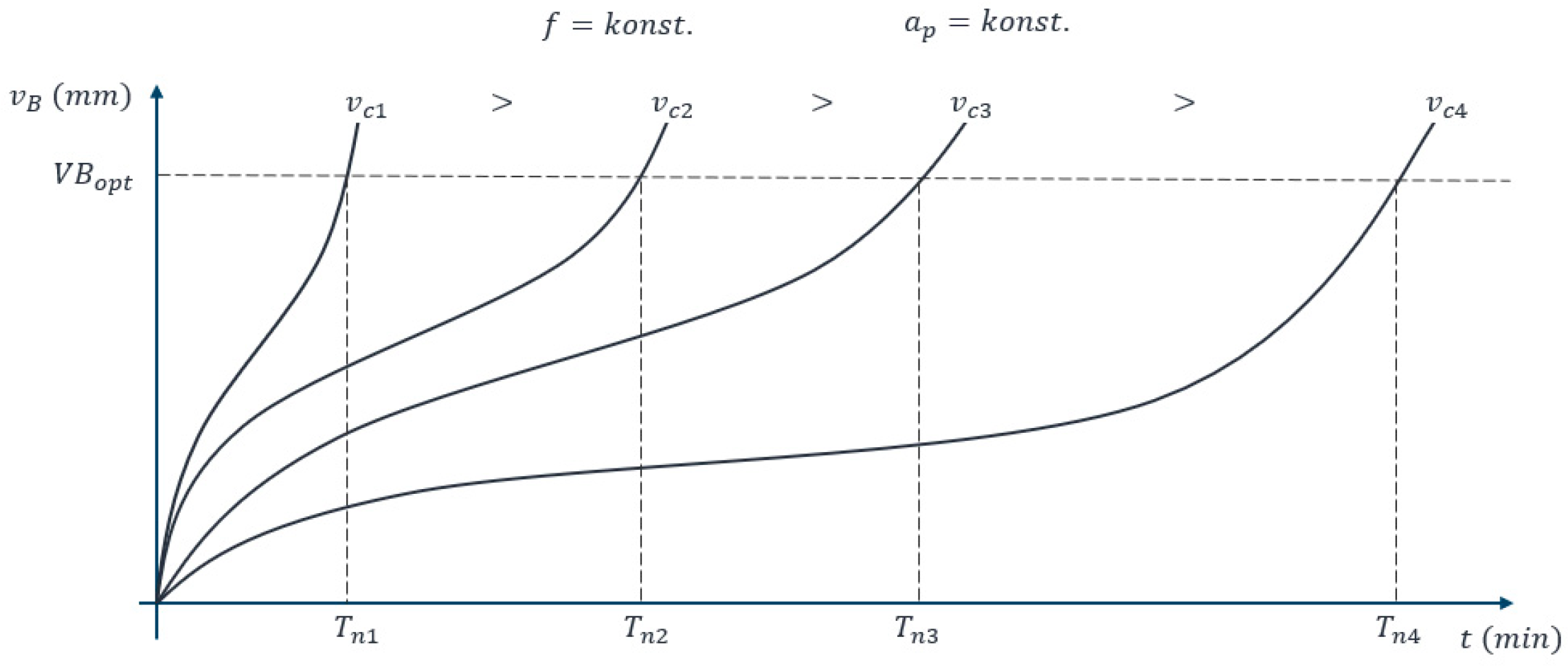
2.1. Tool Wear Detection
2.2. Current-Based Component Wear Detection
2.3. Self-Adapting Digital Twins
2.4. Data Transfer for Digital Twins
- (a)
- Direct data flow from the data source into the Digital Twin;
- (b)
- Indirect data flow from the data source through a processing step into the Digital Twin.
3. Proposed Method
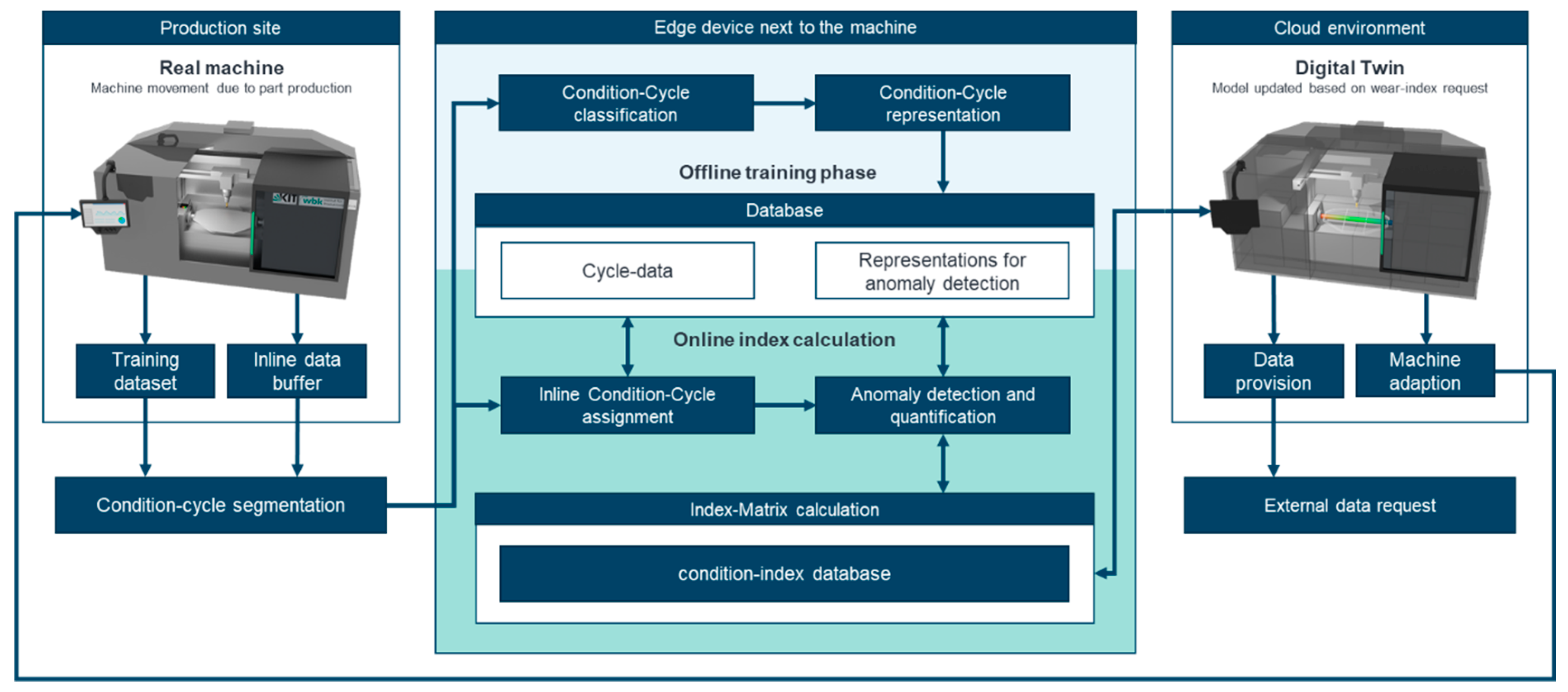
3.1. Concept
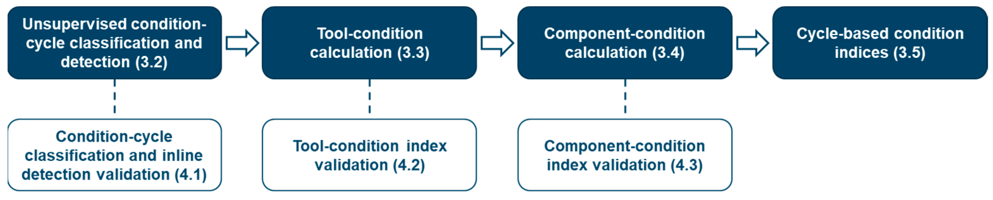
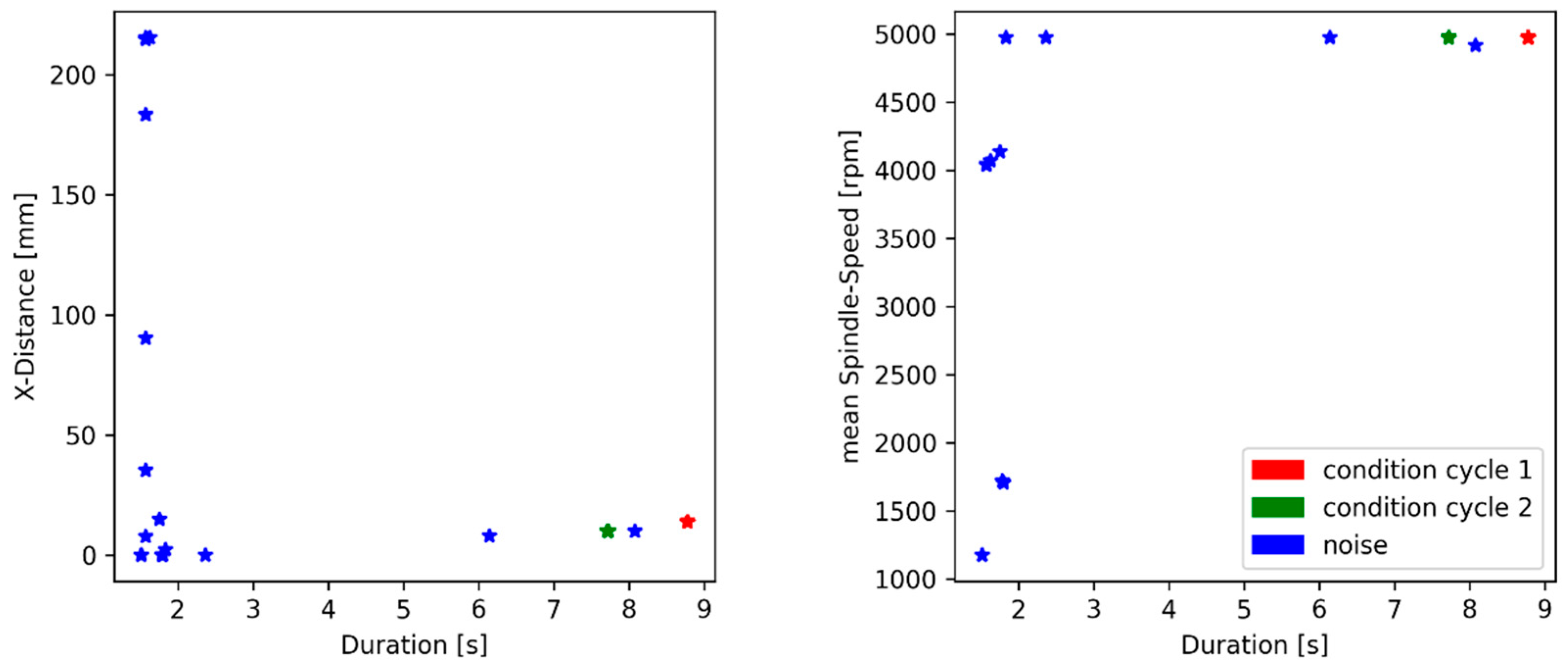
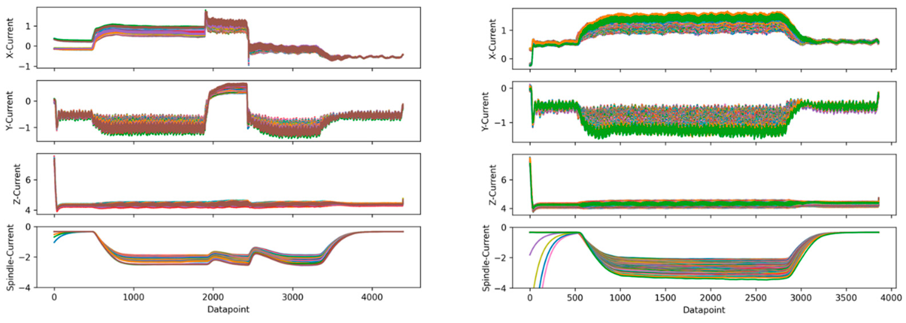
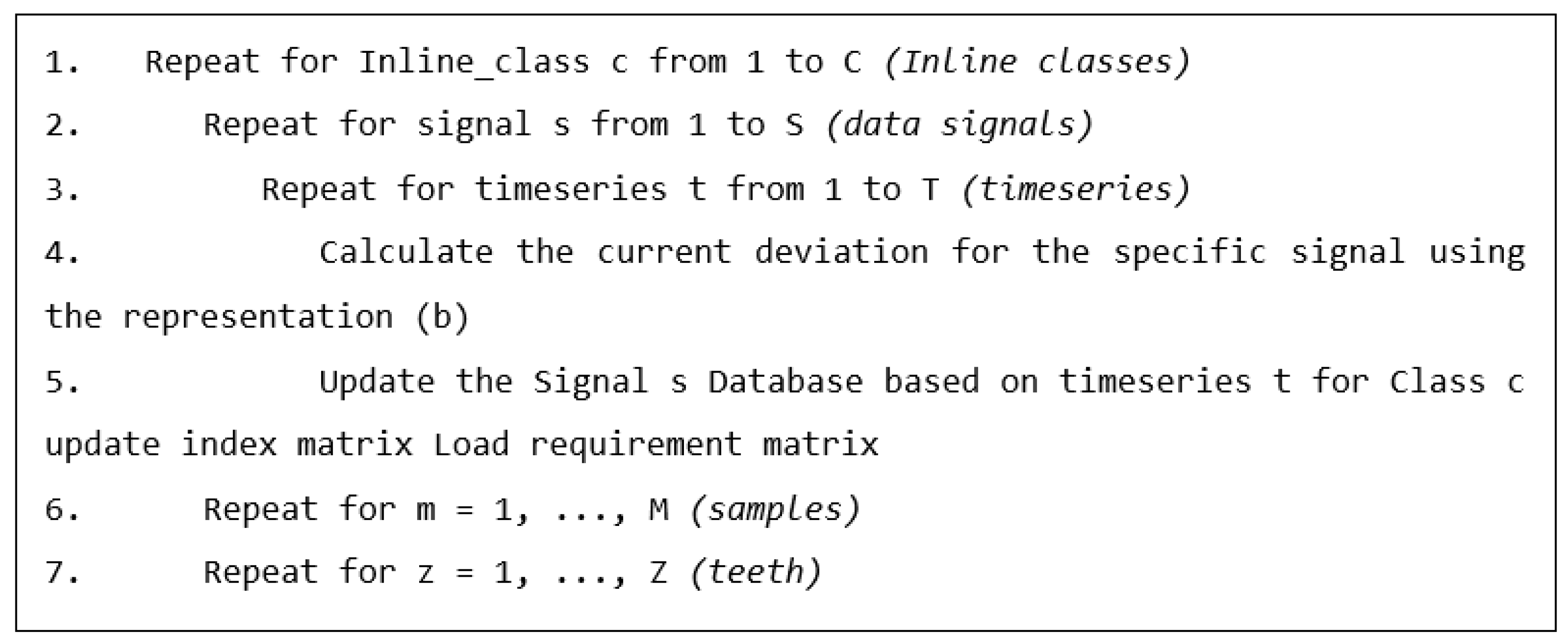
3.2. Unsupervised Condition-Cycle Classification and Detection
3.3. Tool Condition Calculation
3.4. Component Condition Calculation


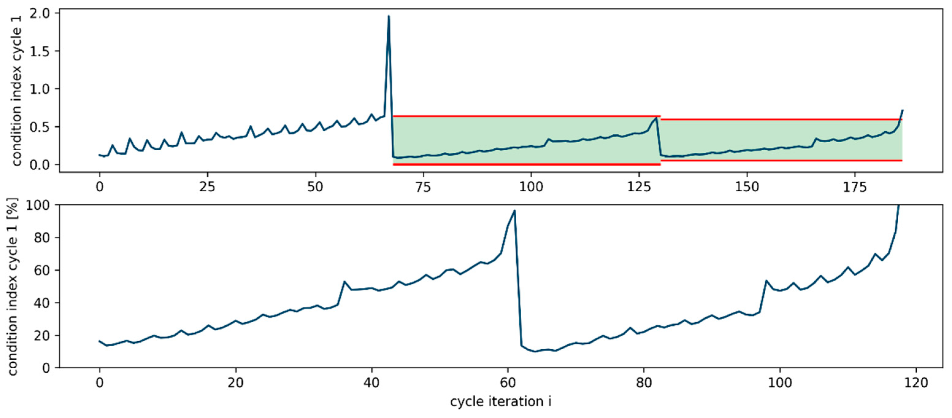
3.5. Cycle-Based Condition Indices
4. Validation
4.1. Condition Cycle Classification and Inline Detection
4.2. Tool Condition Index
4.3. Component Condition Index
5. Discussion
5.1. Wear-Cycle Detection
5.2. Tool Wear Detection
5.3. Component Wear Detection
5.4. Cycle-Based Two-Stage Tool and Component Condition Index
6. Conclusions and Outlook
Author Contributions
Funding
Data Availability Statement
Conflicts of Interest
Abbreviations
| Parameter | Value |
| IPC | Industrial PC |
| Spindle current threshold for relevant sections | |
| Axis position derivative threshold for a relevant section | |
| Number of condition cycles used for the reference | |
| Length of a condition cycle | |
| deviation measure a | Mean value |
| deviation measure b | The mean distance between the data points |
| deviation measure c | Autoencoder reconstruction error |
| condition index calculation for the tool in condition cycle | |
| condition index calculation | |
| Condition-cycle number | |
| Axis or spindle reference, | |
| Weight for the deviation of component during tool run | |
| Current deviation for component in cycle during the Condition index calculation | |
| Lifecycle of a tool | |
| Threshold for tool replacement indicating a recalculation | |
| Ratio factor for the weight recalculation | |
| Spearman correlation | |
| Correlation exponent | |
| Lower tool condition threshold | |
| Upper tool condition threshold | |
| Second derivatives for component in condition cycle during using the local minimum | |
| Second derivatives for component in condition cycle during using the local maximum | |
| Threshold for a change from stage 0 to 1 | |
| Threshold for a change from stage 1 to 2 | |
| Threshold for a change from stage 2 to 3 | |
| Percentage for a change from stage 0 to 1 | |
| Percentage for a change from stage 1 to 2 | |
| Percentage for a change from stage 2 to 3 |
References
- Xu, X. Machine Tool 4.0 for the new era of manufacturing. Int. J. Adv. Manuf. Technol. 2017, 92, 1893–1900. [Google Scholar] [CrossRef]
- Iglesias, A.; Taner Tunç, L.; Özsahin, O.; Franco, O.; Munoa, J.; Budak, E. Alternative experimental methods for machine tool dynamics identification: A review. Mech. Syst. Signal Process. 2022, 170, 108837. [Google Scholar] [CrossRef]
- Rüßmann, M.; Lorenz, M.; Gerbert, P.; Waldner, M.; Justus, J.; Engel, P.; Harnisch, M. Industry 4.0: The Future of Productivity and Growth in Manufacturing Industries. 2015. Available online: https://inovasyon.org/images/Haberler/bcgperspectives_Industry40_2015.pdf (accessed on 16 February 2023).
- Chabanet, S.; El-Haouzi, H.B.; Thomas, P. Toward a self-adaptive Digital Twin based Active learning method: An application to the lumber industry. IFAC-PapersOnLine 2022, 55, 378–383. [Google Scholar] [CrossRef]
- Dalibor, M.; Michael, J.; Rumpe, B.; Varga, S.; Wortmann, A. Towards a Model-Driven Architecture for Interactive Digital Twin Cockpits. In Proceedings of the International Conference on Conceptual Modeling, Vienna, Austria, 3–6 November 2020; Springer: Cham, Switzerland, 2020; pp. 377–387. [Google Scholar]
- Cook, A.A.; Misirli, G.; Fan, Z. Anomaly Detection for IoT Time-Series Data: A Survey. IEEE Internet Things J. 2020, 7, 6481–6494. [Google Scholar] [CrossRef]
- Seevers, J.-P.; Johst, J.; Weiß, T.; Meschede, H.; Hesselbach, J. Automatic Time Series Segmentation as the Basis for Unsupervised, Non-Intrusive Load Monitoring of Machine Tools. Procedia CIRP 2019, 81, 695–700. [Google Scholar] [CrossRef]
- Netzer, M.; Palenga, Y.; Goennheimer, P.; Fleischer, J. Offline-Online pattern recognition for enabling time series anomaly detection on older NC machine tools. J. Mach. Eng. 2021, 21, 98–108. [Google Scholar] [CrossRef]
- Netzer, M.; Palenga, Y.; Fleischer, J. Machine tool process monitoring by segmented timeseries anomaly detection using subprocess-specific thresholds. Prod. Eng. Res. Devel. 2022, 16, 597–606. [Google Scholar] [CrossRef]
- Putz, M.; Frieß, U.; Wabner, M.; Friedrich, A.; Zander, A.; Schlegel, H. State-based and Self-adapting Algorithm for Condition Monitoring. Procedia CIRP 2017, 62, 311–316. [Google Scholar] [CrossRef]
- Jove, E.; Casteleiro-Roca, J.-L.; Quintián, H.; Méndez-Pérez, J.A.; Calvo-Rolle, J.L. A fault detection system based on unsupervised techniques for industrial control loops. Expert Syst. 2019, 36, e12395. [Google Scholar] [CrossRef]
- Theumer, P.; Zeiser, R.; Trauner, L.; Reinhart, G. Anomaly detection on industrial time series for retaining energy efficiency. Procedia CIRP 2021, 99, 33–38. [Google Scholar] [CrossRef]
- Christ, M.; Kempa-Liehr, A.W.; Feindt, M. Distributed and parallel time series feature extraction for industrial big data applications. Neurocomputing 2017, 307, 72–77. [Google Scholar] [CrossRef]
- Zhang, Z.; Wu, X.; Liu, T.; Liu, X. Fault diagnosis of planetary gear backlash based on motor current and Fisher criterion optimized sparse autoencoder. Proc. Inst. Mech. Eng. Part C J. Mech. Eng. Sci. 2022, 236, 7529–7545. [Google Scholar] [CrossRef]
- Teti, R.; Jemielniak, K.; O’Donnell, G.; Dornfeld, D. Advanced monitoring of machining operations. CIRP Ann. 2010, 59, 717–739. [Google Scholar] [CrossRef]
- Hatt, O.; Crawforth, P.; Jackson, M. On the mechanism of tool crater wear during titanium alloy machining. Wear 2017, 374–375, 15–20. [Google Scholar] [CrossRef]
- Siddhpura, A.; Paurobally, R. A review of flank wear prediction methods for tool condition monitoring in a turning process. Int. J. Adv. Manuf. Technol. 2013, 65, 371–393. [Google Scholar] [CrossRef]
- Twardowski, P.; Tabaszewski, M.; Wiciak-Pikuła, M.; Felusiak-Czyryca, A. Identification of tool wear using acoustic emission signal and Machine Learning methods. Precis. Eng. 2021, 72, 738–744. [Google Scholar] [CrossRef]
- Gouarir, A.; Martínez-Arellano, G.; Terrazas, G.; Benardos, P.; Ratchev, S. In-process Tool Wear Prediction System Based on Machine Learning Techniques and Force Analysis. Procedia CIRP 2018, 77, 501–504. [Google Scholar] [CrossRef]
- Neslušan, M.; Turek, S.; Brychta, J.; Čep, R.; Tabaček, M. Experimental methods in splinter machining. EDIS ŽU Žilina 2007, 343. Available online: https://scholar.google.com/citations?user=ipt-r1qaaaaj&hl=de&oi=sra (accessed on 15 February 2023).
- Wang, G.F.; Yang, Y.W.; Zhang, Y.C.; Xie, Q.L. Vibration sensor based tool condition monitoring using ν support vector machine and locality preserving projection. Sens. Actuators A Phys. 2014, 209, 24–32. [Google Scholar] [CrossRef]
- Bergs, T.; Holst, C.; Gupta, P.; Augspurger, T. Digital image processing with deep learning for automated cutting tool wear detection. Procedia Manuf. 2020, 48, 947–958. [Google Scholar] [CrossRef]
- Drouillet, C.; Karandikar, J.; Nath, C.; Journeaux, A.-C.; El Mansori, M.; Kurfess, T. Tool life predictions in milling using spindle power with the neural network technique. J. Manuf. Process. 2016, 22, 161–168. [Google Scholar] [CrossRef]
- Zhou, Y.; Sun, W. Tool Wear Condition Monitoring in Milling Process Based on Current Sensors. IEEE Access 2020, 8, 95491–95502. [Google Scholar] [CrossRef]
- Walther, M. Antriebsbasierte Zustandsdiagnose von Vorschubantrieben. Ph.D. Thesis, University of Stuttgart, Stuttgart, Germany, 2011. Heimsheim: Jost-Jetter (ISW/IPA Forschung und Praxis, 183). [Google Scholar]
- Han, Y.; Song, Y.H. Condition monitoring techniques for electrical equipment-a literature survey. IEEE Trans. Power Deliv. 2003, 18, 4–13. [Google Scholar] [CrossRef]
- Corne, B.; Knockaert, J.; Desmet, J. Misalignment and unbalance fault severity estimation using stator current measurements. In Proceedings of the IEEE 11th International Symposium on Diagnostics for Electrical Machines, Power Electronics and Drives (SDEMPED), Tinos, Greece, 29 August–1 September 2017. [Google Scholar]
- Nguyen, T.L.; Ro, S.-K.; Park, J.-K. Study of ball screw system preload monitoring during operation based on the motor current and screw-nut vibration. Mech. Syst. Signal Process. 2019, 131, 18–32. [Google Scholar] [CrossRef]
- Jamshidi, M.; Chatelain, J.-F.; Rimpault, X.; Balazinski, M. Tool condition monitoring based on the fractal analysis of current and cutting force signals during CFRP trimming. Int. J. Adv. Manuf. Technol. 2022, 121, 8127–8142. [Google Scholar] [CrossRef]
- Czichos, H. Tribologie-Handbuch. Tribometrie, Tribomaterialien, Tribotechnik; überarbeitete und erweiterte Auflage; Vieweg+Teubner: Wiesbaden, Germany, 2010. [Google Scholar]
- Zhao, J.; Lin, M.; Song, X.; Guo, Q. Analysis of the precision sustainability of the preload double-nut ball screw with consideration of the raceway wear. Proc. Inst. Mech. Eng. Part J J. Eng. Tribol. 2020, 234, 1530–1546. [Google Scholar] [CrossRef]
- Sato, R. Wear Estimation of Ball Screw and Support Bearing Based on Servo Signals in Feed Drive System. In Proceedings of the International Conference on Leading Edge Manufacturing in 21st Century, Nagoya, Japan, 19–22 October 2011; Volume 6, p. _3233-1_. [Google Scholar]
- Liu, X.; Mao, X.; He, Y.; Liu, H.; Fan, W.; Li, B. A new approach to identify the ball screw wear based on feed motor current. In Proceedings of the International Conference on Artificial Intelligence and Robotics and the International Conference on Automation, Control and Robotics Engineering, Kitakyushu, Japan, 13–15 July 2016; ACM: New York, NY, USA, 2016. [Google Scholar]
- Yang, Q.; Li, X.; Wang, Y.; Ainapure, A.; Lee, J. Fault Diagnosis of Ball Screw in Industrial Robots Using Non-Stationary Motor Current Signals. Procedia Manuf. 2020, 48, 1102–1108. [Google Scholar] [CrossRef]
- Kritzinger, W.; Karner, M.; Traar, G.; Henjes, J.; Sihn, W. Digital Twin in manufacturing: A categorical literature review and classification. IFAC-PapersOnLine 2018, 51, 1016–1022. [Google Scholar] [CrossRef]
- Bibow, P.; Dalibor, M.; Hopmann, C.; Mainz, B.; Rumpe, B.; Schmalzing, D. Model-Driven Development of a Digital Twin for Injection Molding. In Proceedings of the International Conference on Advanced Information Systems Engineering, Grenoble, France, 8–12 June 2020; Springer: Cham, Switzerland, 2020; pp. 85–100. Available online: https://link.springer.com/chapter/10.1007/978-3-030-49435-3_6 (accessed on 1 March 2023).
- Bolender, T.; Burvenich, G.; Dalibor, M.; Rumpe, B.; Wortmann, A. Self-Adaptive Manufacturing with Digital Twins. In Proceedings of the International Symposium on Software Engineering for Adaptive and Self-Managing Systems (SEAMS), Madrid, Spain, 18–24 May 2021. [Google Scholar]
- Hribernik, K.; Cabri, G.; Mandreoli, F.; Mentzas, G. Autonomous, context-aware, adaptive Digital Twins—State of the art and roadmap. Comput. Ind. 2021, 133, 103508. [Google Scholar] [CrossRef]
- Uhlemann, T.H.-J.; Schock, C.; Lehmann, C.; Freiberger, S.; Steinhilper, R. The Digital Twin: Demonstrating the Potential of Real Time Data Acquisition in Production Systems. Procedia Manuf. 2017, 9, 113–120. [Google Scholar] [CrossRef]
- Costantini, A.; Di Modica, G.; Ahouangonou, J.C.; Duma, D.C.; Martelli, B.; Galletti, M. IoTwins: Toward Implementation of Distributed Digital Twins in Industry 4.0 Settings. Computers 2022, 11, 67. [Google Scholar] [CrossRef]
- D’Agostino, D.; Morganti, L.; Corni, E.; Cesini, D.; Merelli, I. Combining Edge and Cloud computing for low-power, cost-effective metagenomics analysis. Future Gener. Comput. Syst. 2019, 90, 79–85. [Google Scholar] [CrossRef]
- Asim, M.; Wang, Y.; Wang, K.; Huang, P.-Q. A Review on Computational Intelligence Techniques in Cloud and Edge Computing. IEEE Trans. Emerg. Top. Comput. Intell. 2020, 4, 742–763. [Google Scholar] [CrossRef]
- Shi, W.; Cao, J.; Zhang, Q.; Li, Y.; Xu, L. Edge Computing: Vision and Challenges. IEEE Internet Things J. 2016, 3, 637–646. [Google Scholar] [CrossRef]
- Hu, L.; Nguyen, N.-T.; Tao, W.; Leu, M.C.; Liu, X.F.; Shahriar, M.R.; Al Sunny, S.M.N. Modeling of Cloud-Based Digital Twins for Smart Manufacturing with MT Connect. Procedia Manuf. 2018, 26, 1193–1203. [Google Scholar] [CrossRef]
- Jiang, Y.; Yin, S.; Li, K.; Luo, H.; Kaynak, O. Industrial applications of Digital Twins. Philos. Trans. Ser. A Math. Phys. Eng. Sci. 2021, 379, 20200360. [Google Scholar] [CrossRef] [PubMed]
- Salgado, D.R.; Alonso, F.J. An approach based on current and sound signals for in-process tool wear monitoring. Int. J. Mach. Tools Manuf. 2007, 47, 2140–2152. [Google Scholar] [CrossRef]
- Schubert, E.; Sander, J.; Ester, M.; Kriegel, H.P.; Xu, X. DBSCAN Revisited. ACM Trans. Database Syst. 2017, 42, 19. [Google Scholar] [CrossRef]
- Zhang, C.; Liu, J.; Chen, W.; Shi, J.; Yao, M.; Yan, X.; Xu, N.; Chen, D. Unsupervised anomaly detection based on deep autoencoding and clustering. Secur. Commun. Netw. 2021, 2021, 7389943. [Google Scholar] [CrossRef]
- Netzer, M. Intelligente Anomalieerkennung für Hochflexible Produktionsmaschinen: Prozessüberwachung in der Brownfield Produktion. Ph.D. Thesis, Karlsruhe Institute of Technology, Karlsruhe, Germany, 2022. [Google Scholar]
- 50. Zhang, L.; Gao, H.; Dong, D.; Fu, G.; Liu, Q. Wear Calculation-Based Degradation Analysis and Modeling for Remaining Useful Life Prediction of Ball Screw. Math. Probl. Eng. 2018, 2018, 2969854. [Google Scholar] [CrossRef]


| Corr (a,b) | Corr (b,c) | Corr (c,b) | |
|---|---|---|---|
| 1 x-axis | −0.04939276 | −0.16543531 | −0.91010147 |
| 1 y-axis | −0.95581863 | −0.98985663 | 0.94993983 |
| 1 z-axis | −0.70774908 | 0.97707274 | −0.76128193 |
| 1 spindle | −0.99934485 | −0.99784553 | 0.99735604 |
| 2 x-axis | −0.49271491 | 0.50516899 | −0.85388119 |
| 2 y-axis | −0.76455602 | −0.81543437 | 0.63313464 |
| 2 z-axis | −0.98536464 | 0.54104406 | −0.53004049 |
| 2 spindle | −0.99961592 | −0.9941404 | 0.99477251 |
| 3 x-axis | −0.75277514 | 0.59002364 | −0.70386803 |
| 3 y-axis | −0.96254714 | −0.96116497 | 0.93236389 |
| 3 z-axis | −0.99820867 | −0.52270938 | 0.52980505 |
| 3 spindle | −0.99970386 | 0.97345975 | −0.97130338 |
| Area Transition | Condition | Percentage |
|---|---|---|
| 0 to 1 | ||
| 1 to 2 | ||
| 2 to 3 |
Disclaimer/Publisher’s Note: The statements, opinions and data contained in all publications are solely those of the individual author(s) and contributor(s) and not of MDPI and/or the editor(s). MDPI and/or the editor(s) disclaim responsibility for any injury to people or property resulting from any ideas, methods, instructions or products referred to in the content. |
© 2023 by the authors. Licensee MDPI, Basel, Switzerland. This article is an open access article distributed under the terms and conditions of the Creative Commons Attribution (CC BY) license (https://creativecommons.org/licenses/by/4.0/).
Share and Cite
Ströbel, R.; Bott, A.; Wortmann, A.; Fleischer, J. Monitoring of Tool and Component Wear for Self-Adaptive Digital Twins: A Multi-Stage Approach through Anomaly Detection and Wear Cycle Analysis. Machines 2023, 11, 1032. https://doi.org/10.3390/machines11111032
Ströbel R, Bott A, Wortmann A, Fleischer J. Monitoring of Tool and Component Wear for Self-Adaptive Digital Twins: A Multi-Stage Approach through Anomaly Detection and Wear Cycle Analysis. Machines. 2023; 11(11):1032. https://doi.org/10.3390/machines11111032
Chicago/Turabian StyleStröbel, Robin, Alexander Bott, Andreas Wortmann, and Jürgen Fleischer. 2023. "Monitoring of Tool and Component Wear for Self-Adaptive Digital Twins: A Multi-Stage Approach through Anomaly Detection and Wear Cycle Analysis" Machines 11, no. 11: 1032. https://doi.org/10.3390/machines11111032