Article

Kinematic Models and the Performance Level Index of a Picking-and-Placing Hybrid Robot

1
Lassonde School of Engineering, York University, Toronto, ON M3J 1P3, Canada
2
Department of Mechanical Engineering, The Hong Kong Polytechnic University, Hung Hom, Kowloon, Hong Kong
3
Intelligent Robotics Research Center, Zhejiang Lab, Hangzhou 311100, China
*
Author to whom correspondence should be addressed.
Machines 2023, 11(10), 979; https://doi.org/10.3390/machines11100979
Submission received: 9 October 2023 / Revised: 20 October 2023 / Accepted: 20 October 2023 / Published: 23 October 2023
(This article belongs to the Special Issue New Trends in Robotics and Automation)

Abstract

:
The mobile platform of the parallel robot designed for picking and placing operations is usually equipped with one or two extra degree(s) of freedom to enable flexible grasping orientations. However, additional motors indicate extra loads for the moving platform, and the total payload performance shrinks. This paper proposes a spatial picking-and-placing manipulator, in which one actuator that is supposed to be installed on the mobile platform is placed far away from the mobile platform. The platform has a large workspace along one direction. The comprehensive analytical inverse and forward kinematic solutions of this robot are derived. The reachable workspace of the parallel manipulator module is then explored. The novel performance level index is designed to normalize the performance index and demonstrate the performance rank for any pose. A mathematical proof is provided for this novel index. The manipulability index is taken as an example to examine the level indicator. A multi-objective optimization is implemented to pursue optimal performance; then, the initial design and optimized results are compared in detail. A sample trajectory is provided to verify the correctness of the kinematic mathematical model of the parallel mechanism.

1. Introduction

The products in picking and placing applications may have various shapes, sizes, weights, surface stiffness, positions and orientations, and complex stacking manners [1,2,3]. Hence, grippers are required to possess large reachable and dexterous workspaces in order to have flexible capabilities. Another essential condition is high speed and acceleration to improve operation efficiency, which makes this kind of task more complicated [4,5].
Apparently, a parallel-structure-based robot can conduct pick-and-place operations according to its intrinsic characteristics [6]. The Delta robot invented by Reymond Clavel [7] was equipped with 3-R(S-S)2 parallel structure (R is the rotary pair, and S indicates a spherical joint). It possessed a three-dimensional (3D) translational workspace and was widely employed in various picking-and-placing operations [8,9,10]. Belzile et al. [11] explored a 2-CRRH (C and H indicate, respectively, cylindrical and helical joints) parallel architecture for pick-and-place operations. The moving platform could achieve Schönflies motion in space with a premium limitless rotational capability. The X4 robot 4-R(S-S)2R was outlined in [12]. This robot could generate 3T1R (three translations and one rotation). An exhaustive study on the kinematic analysis was expressed, based upon which the optimal design was established. Furthermore, its dynamic performance evaluations and power consumption analysis were conducted in [13,14]. Rahul et al. [15] designed a two-degree-of-freedom (DOF) planar parallel robot to automatically load/unload paper pot seedlings in agriculture applications. This robot was equipped with five revolute joints, and most linkages were manufactured via 3D printing. The same kind of five-bar linkage mechanism was also mentioned in [16]. It was upgraded and named DexTAR, which exhibited high accuracy. Its four groups of operation modes, interference areas, and singularity loci were determined comprehensively. Similarly to H4 and I4R parallel robots, the Par4 parallel architecture with symmetrical features and an articulated mobile platform was introduced in [17]. This novel design could avoid the shortcomings of these previous robots and still possess high speed and acceleration. Briot and Bonev [18] developed a spatial parallel robot, Pantopteron, with pure sliding movements aimed at pick-and-place tasks. Its three DOFs were completely decoupled. It could realize high speeds and large reachable workspace due to the unique pantograph linkage mechanism installed in each kinematic branch.
Designing a picking-and-placing parallel robot with extraordinary strokes along one axis is still challenging, not to mention the requirement of a large workspace in all directions. Considering the different robot structures of serial and parallel robots, a serial–parallel hybrid robot may be an option for meeting the requirements of picking-and-placing operations.
In addition, the performance evaluation of parallel architecture is essential in order to make full use of its intrinsic advantages. A generalized articulated parallel manipulator (RRPaR)2-R-(RRPaRR)2 (Pa denotes parallelogram linkage) was established in [19]. Beyond the kinematic mathematic models and kinematic performance evaluations, a special workspace that was far from singularity configurations was selected as the operational workspace. The parallel diamond structure was reported in [20]. The rotary movement of the mobile platform was constrained due to the parallelogram mechanism in each kinematic limb. Detailed kinematic performance analyses, including workspace and dexterity analyses, were conducted. During the designing phase, the force transmission property was considered to be more suitable for battery assembly lines. Its global kinematic constraints and dynamic performance were further evaluated in [21]. A solar tracker based on the U/PRU/PUS (P and U represent prismatic and universal joints, respectively) parallel robot was designed in [22]. The two-axis rotational workspace/area of this device was computed and employed as the optimization target in dimensional synthesis. In the work of [23], the maximum orientation capacity and the global transmission and constraint index for parallel manipulators were deduced. Both were examined in a group of parallel robots: 3-UCR and 3-RCU (C indicates cylindrical joints). The novel dynamic transfer performance index and dynamic transfer balance performance index were defined in [24]. Better performances could be obtained using a larger former index and a smaller latter index. These indices were further employed as optimization objects in the trajectory planning of a hybrid robot. An end-effector transmission index and branch transmission index were proposed in [25]. The authors further brought forward a special local transmission index based on orthogonal degrees. This index was evaluated on a planar 2-DOF parallel robot with various driving modes. To avoid the singularity problem of the Jacobian matrix, the kinetostatic conditioning index was proposed in [26,27]. The designed index was not dependent on the configuration of the parallel robot. Patel and Sobh [28] investigated and concluded the widely used performance indices of parallel mechanisms. In this research study, thirty-six indices were sorted with respect to three methods: the local or global index, the kinematic or dynamic index or neither, and the intrinsic or extrinsic index. Brinker et al. [29] conducted an exhaustive study on kinematic performance indices for parallel structures. Both the advantages and shortcomings of the condition number, manipulability index, and motion/force transmission index were discussed in detail. The solutions for overcoming the limitations of Jacobian-matrix-based indices were provided.
These various indices can provide a more comprehensive understanding with respect to evaluating serial/parallel/hybrid robots. A concern arises with respect to how one can deal with many different categories of performance indices, kinematic/dynamic indices, and performance indices with various ranges. It is also difficult to clarify that one pose of a robot is superior to one specific pose of another robot relative to a given performance measure. The performance ranking of any pose within a reachable workspace is unknown.
Considering the above two main problems, a novel hybrid robot with a large workspace along one direction is proposed in this research study. A novel index is explored to normalize any performance index and provide performance ratings for each position/orientation within the workspace. The article is arranged as follows: the structural design of this robot is presented in Section 2, and it is followed by Section 3, which formulates the analytical kinematic relations. The workspace’s analysis and novel level index are investigated in Section 4. Multi-objective linkage optimization and performance comparisons are conducted in Section 5. A case study is shown in Section 6, and the conclusions are provided in Section 7.

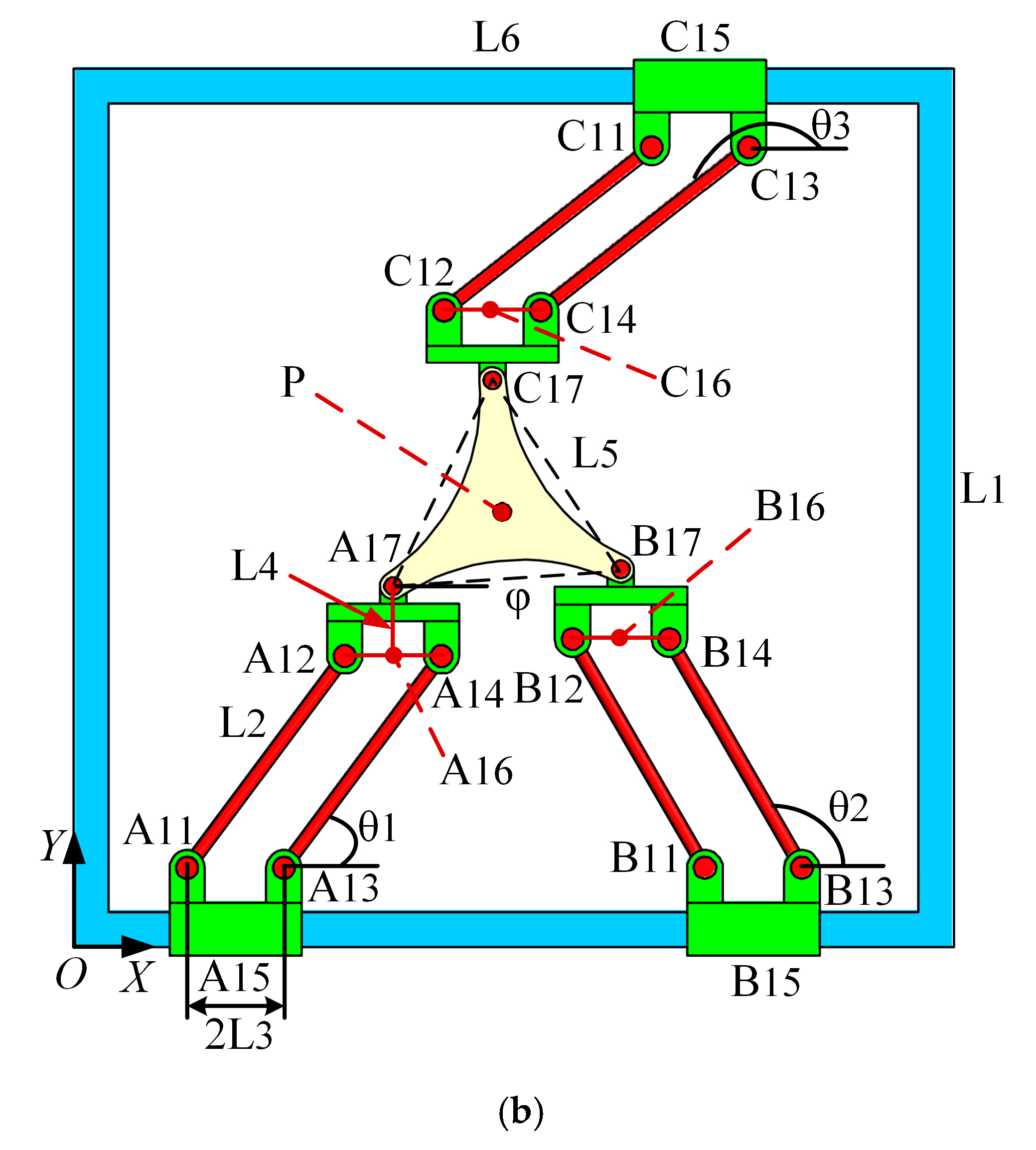
2. Mechanical Design

A hybrid manipulator employed for the picking-and-placing operation is proposed, as shown in Figure 1a. This hybrid structure comprises a planar parallel mechanism [30] (shown in Figure 1b), a belt drive system, a rack and pinion module, and a gripper. The coordinate system is located at the bottom left corner, as illustrated in Figure 1b. Based on the right-hand rule, the Z-axis is perpendicular to the XOY plane and points outward.
This parallel robot includes one fixed platform and a mobile platform connected by three independent kinematic chains. Each chain comprises one active prismatic joint, one parallelogram joint ((R-R)2 linkage), and a revolute joint. All sliding joints move along the X direction, and this linear motion can be realized using a lead screw motion system. The parallelogram joints are placed on the XOY plane. In each kinematic branch, one side of the parallelogram joint is installed on the driving sliding joint, and another side is attached to the moving platform with a rotary joint. The axes of the three rotational joints connected to the mobile platform are all parallel relative to the Z-axis.
Points A16, B16, and C16 are the midpoints of A12A14, B12B14, and C12C14, respectively. Pulley-a is placed at the midpoint of A11A13. Pulley-b and pulley-c both comprise two pulleys. They are separately mounted on points A16 and A17. The shafts of the aforementioned three pulleys are colinear with the Z-axis. Pulley-d is installed on the moving platform, and its axis is perpendicular to the Z-axis. Pulley-a drives pulley-b through belt-a. Pulley-b and pulley-c are linked by belt-b. Pulley-c and pulley-d are connected by belt-c.
The spur gear is fixed to pulley-d, and they share the same rotational axis. The rack matching the spur gear can slide along the Z direction with respect to the mobile platform. The rack is installed vertically at the center of the mobile platform. The gripper is fixed at the bottom end of the rack. The movement of pulley-a manipulates the translation of the gripper.
Although a motor directly installed on the mobile platform can drive the spur gear, this is avoided in this research study. One of the reasons is that a compact moving platform can be enabled. A remote actuator would make the moving platform geometrically more compact. Another concern is the inertial property. The mobile platform with three movements requires a larger mass in order to attach the actuator with the large mass feature. In this case, the inertia features of the mobile platform and the actuator are enlarged. The high-speed performance of the parallel robot module is affected. The requirements for the other three sliding actuators are improved under the same payload conditions. Therefore, this actuator for Z-direction translation is installed far from the mobile platform. The corresponding transmission parts are designed using lightweight structures and materials.
This planar parallel architecture can achieve two translations along the X-axis and Y-axis and one rotational movement about the Z-axis. The belt drive system and the gear rack system enable the gripper to translate along the Z direction. In summary, the entire hybrid robot has four DOFs.

3. Kinematic Solutions

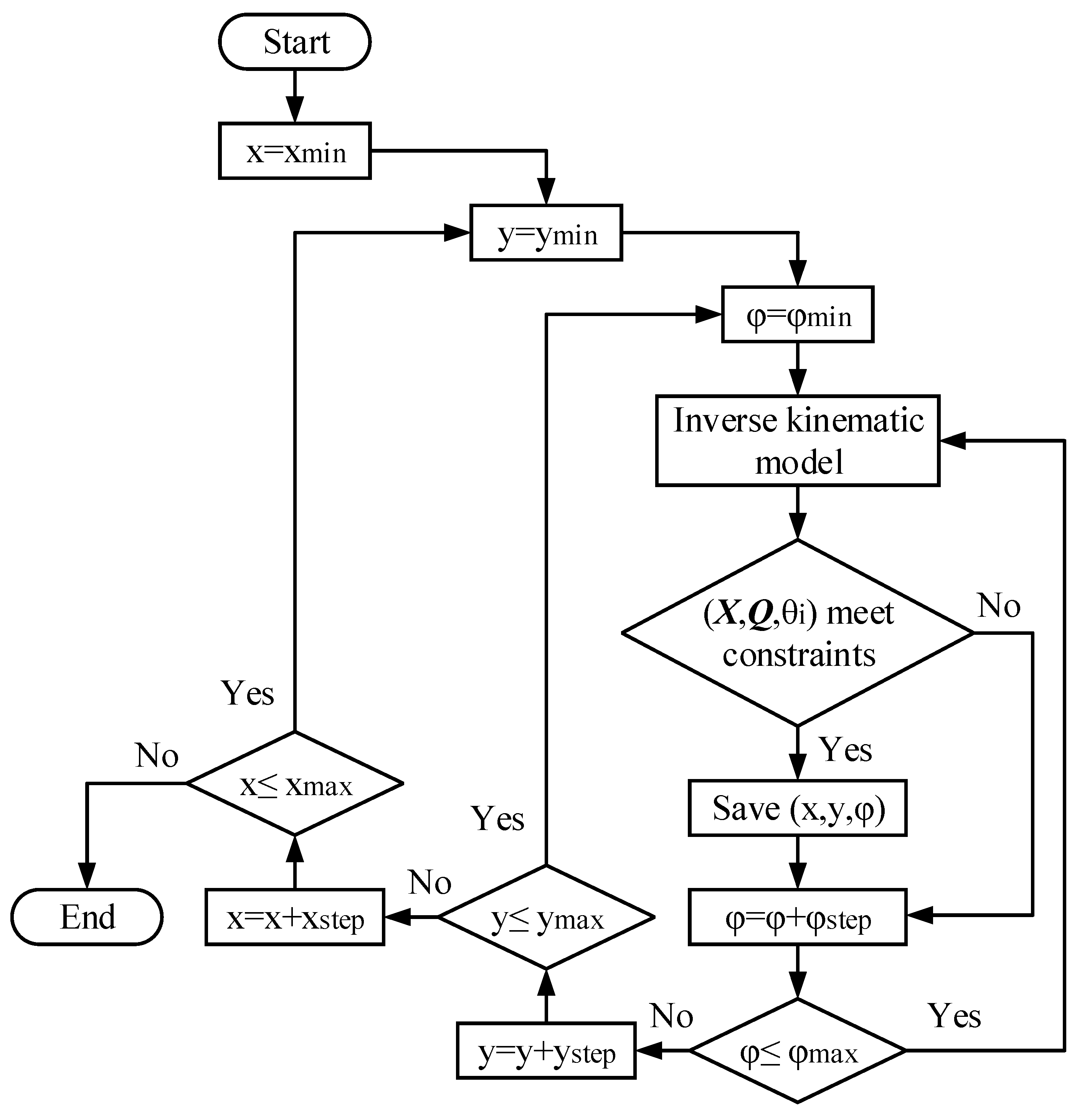
3.1. Inverse Kinematics of the Parallel Robot

The detailed linkage dimensions of the parallel manipulator with three identical chains are also illustrated in Figure 1b. The fixed platform is a rectangle with a length of L1 and width of L6. A 11 A 12 = A 13 A 14 = L 2 . A 11 A 13 = A 12 A 14 = 2 L 3 . A 16 A 17 = L 4 . The corresponding linkages of the three chains have the same dimensions. Mobile platform A17B17C17 forms a virtual equilateral triangle with an edge of L5, and its center is point P. According to the features of this triangle, A 17 P = B 17 P = C 17 P = 3 L 5 / 3 . The positions along the X direction of active sliding joints A15, B15, and C15 are x1, x2, and x3, respectively. The system input of this parallel manipulator is defined as Q = [ x 1 , x 2 , x 3 ] T . The sloping angles between the positive X-axis and linkages A13A14, B13B14, and C13C14 are, respectively, denoted as θ 1 , θ 2 , and θ 3 . The angle between the virtual edge A17B17 and the positive X-axis is φ . The position of point P in the provided coordinate system is (x, y). Thereafter, the pose of the mobile platform is given as X = [ x , y , φ ] T .
The inverse kinematic problem can be computed with the given X. For the first kinematic chain, the vector-loop equation is obtained as follows:
O A 15 + A 15 A 16 + A 16 A 17 + A 17 P = OP .
Equation (1) can be expressed along two orthogonal directions:
X   a x i s : x 1 + L 2 cos θ 1 + 3 L 5 / 3 cos ( φ + π / 6 ) = x Y   a x i s :   L 2 sin θ 1 + L 4 + 3 L 5 / 3 sin ( φ + π / 6 ) = y .
From Equation (2), unknown parameter θ 1 should be placed on one side while the others are on the other side to eliminate θ 1 . Hence, Equation (2) is rephrased as
L 2 cos θ 1 = x 3 L 5 / 3 cos ( φ + π / 6 ) x 1 L 2 sin θ 1 = y 3 L 5 / 3 sin ( φ + π / 6 ) L 4 .
Adding the squares of both equations in Equation (3) leads to
L 2 2 = x 3 L 5 / 3 cos ( φ + π / 6 ) x 1 2 + y 3 L 5 / 3 sin ( φ + π / 6 ) L 4 2 .
The position of the active prismatic joint A15 is then solved as
x 1 = x 3 L 5 / 3 cos ( φ + π / 6 ) ± L 2 2 y 3 L 5 / 3 sin ( φ + π / 6 ) L 4 2 .
Similar calculation steps for the first branch will be employed for the remaining supporting branches. The closed-loop equations for the other supporting branches are calculated as
O B 15 + B 15 B 16 + B 16 B 17 + B 17 P = OP
O C 15 + C 15 C 16 + C 16 C 17 + C 17 P = OP .
Both Equations (6) and (7) are described in two orthogonal directions, and passive parameters θ 2 and θ 3 are placed on one side, as arranged below.
L 2 cos θ 2 = x 3 L 5 / 3 cos ( φ + 5 π / 6 ) x 2 L 2 sin θ 2 = y 3 L 5 / 3 sin ( φ + 5 π / 6 ) L 4
L 2 cos θ 3 = x 3 L 5 / 3 cos ( φ + 3 π / 2 ) x 3 L 2 sin θ 3 = y 3 L 5 / 3 sin ( φ + 3 π / 2 ) L 1 + L 4 .
Summing the squares of both equations in Equations (8) and (9), the following expressions can be deduced, respectively.
L 2 2 = x 3 L 5 / 3 cos ( φ + 5 π / 6 ) x 2 2 + y 3 L 5 / 3 sin ( φ + 5 π / 6 ) L 4 2
L 2 2 = x 3 L 5 / 3 cos ( φ + 3 π / 2 ) x 3 2 + y 3 L 5 / 3 sin ( φ + 3 π / 2 ) L 1 + L 4 2 . lim x
The positions of remaining actuation joints B15 and C15 can be formulated separately and are listed below.
x 2 = x 3 L 5 / 3 cos ( φ + 5 π / 6 ) ± L 2 2 y 3 L 5 / 3 sin ( φ + 5 π / 6 ) L 4 2
x 3 = x 3 L 5 / 3 cos ( φ + 3 π / 2 ) ± L 2 2 y 3 L 5 / 3 sin ( φ + 3 π / 2 ) L 1 + L 4 2 .
The analytical solution of the inverse kinematic model is concluded in Equations (5), (12) and (13).

3.2. Direct Kinematics of the Parallel Robot

The forward kinematic problem can be calculated using the predefined Q. Equations (4), (10) and (11) can be deduced in the following form:
x 2 + y 2 + e 11 x + e 12 y + e 13 = 0
x 2 + y 2 + e 21 x + e 22 y + e 23 = 0
x 2 + y 2 + e 31 x + e 32 y + e 33 = 0 ,
where
e 11 = 2 3 L 5 / 3 cos ( φ + π / 6 ) + x 1 e 12 = 2 3 L 5 / 3 sin ( φ + π / 6 ) + L 4 e 13 = 3 L 5 / 3 cos ( φ + π / 6 ) + x 1 2 + 3 L 5 / 3 sin ( φ + π / 6 ) + L 4 2 L 2 2
e 21 = 2 3 L 5 / 3 cos ( φ + 5 π / 6 ) + x 2 e 22 = 2 3 L 5 / 3 sin ( φ + 5 π / 6 ) + L 4 e 23 = 3 L 5 / 3 cos ( φ + 5 π / 6 ) + x 2 2 + 3 L 5 / 3 sin ( φ + 5 π / 6 ) + L 4 2 L 2 2
e 31 = 2 3 L 5 / 3 cos ( φ + 3 π / 2 ) + x 3 e 32 = 2 3 L 5 / 3 sin ( φ + 3 π / 2 ) + L 1 L 4 e 33 = 3 L 5 / 3 cos ( φ + 3 π / 2 ) + x 3 2 + 3 L 5 / 3 sin ( φ + 3 π / 2 ) + L 1 L 4 2 L 2 2 .
Subtracting Equation (15) from Equation (14) results in the following:
e 41 x + e 42 y + e 43 = 0 ,
where e 4 i = e 1 i e 2 i i = 1 , 2 , 3 .
Subtracting Equation (16) from Equation (14) generates the following:
e 51 x + e 52 y + e 53 = 0 ,
where e 5 i = e 1 i e 3 i i = 1 , 2 , 3 .
Parameters x and y can be computed by solving Equations (17) and (18):
x = e 62 e 61 ,   y = e 63 e 61 ,
where
e 61 = e 41 e 52 e 42 e 51 e 62 = e 42 e 53 e 43 e 52 e 63 = e 41 e 53 e 43 e 51
Combining Equations (14) and (19) yields
e 62 2 + e 63 2 + e 11 e 61 e 62 e 12 e 61 e 63 + e 13 e 61 2 = 0 .
Hence, variable φ can be computed since it is the only unknown parameter in Equation (20). The tangent half-angle formula can be employed for Equation (20), which is transferred as an eighth-degree polynomial. The polynomial denotes that eight poses at most are obtained with the predefined Q.

3.3. Kinematic Model of Z-Displacement

The initial configuration of the vertical (along the Z direction) translation system is illustrated in Figure 2. Figure 2 is depicted in a two-dimensional plane to clearly state all parameters. The dimensions of this system are described, and the radius of pulley-a is R1. The radii of the two pulleys within pulley-b are R2 and R3. The radii of the two pulleys of pulley-c are R4 and R5. The radius of pulley-d is R6. The pitch diameter of the pinion is defined as 2R7. The rack has a length of L7. In this original assembly configuration, the midpoint of the rack is placed at point P of the moving platform. The bottom point of the rack that is attached to the end-effector is represented as E. It is noteworthy that the x- and y-components of the position of point E are the same as that of point P. The only unknown parameter is the z-component of the displacement of point E.
Once driving pulley-a has a rotation angle of α 1 (shown in Figure 2), the rotary angles for pulley-b, pulley-c, and pulley-d are separately denoted as α 2 , α 3 , and α 4 . All angles are in radians, and the reference line is the X-axis. In accordance with the belt mission, the following expressions can be obtained:
S 1 = α 1 R 1 = α 2 R 2 S 2 = α 2 R 3 = α 3 R 4 S 3 = α 3 R 5 = α 4 R 6 ,
where S1, S2, and S3 denote the displacements of belt-a, belt-b, and belt-c, respectively.
Based on rack–pinion transmission, the height of the rack can be calculated as follows:
z r a c k = α 4 R 7 .
The position of point E is then derived as
z E = z r a c k L 7 / 2 .
Combining Equations (21) and (22), the forward kinematic mathematical solution shown in Equation (23) is further expressed as
z E = R 1 R 3 R 5 R 7 R 2 R 4 R 6 α 1 L 7 / 2 .
The inverse kinematic analytical model of this transmission system can also be formulated using Equation (24), as indicated below.
α 1 = R 2 R 4 R 6 R 1 R 3 R 5 R 7 ( z E + L 7 / 2 ) .

4. Kinematic Performance Assessments

From Figure 1a, the full rotation of pulley-a allows the rack to move along the Z direction, and the corresponding translational range of the four-DOF mechanism is merely dependent on the length of the rack. It is evident that a longer rack enables a larger workspace. It is difficult to achieve such a long stroke along one direction for a traditional parallel mechanism with the same scale. Henceforth, the remaining calculations and discussions are only for the parallel module: the 3-PPaR parallel mechanism.

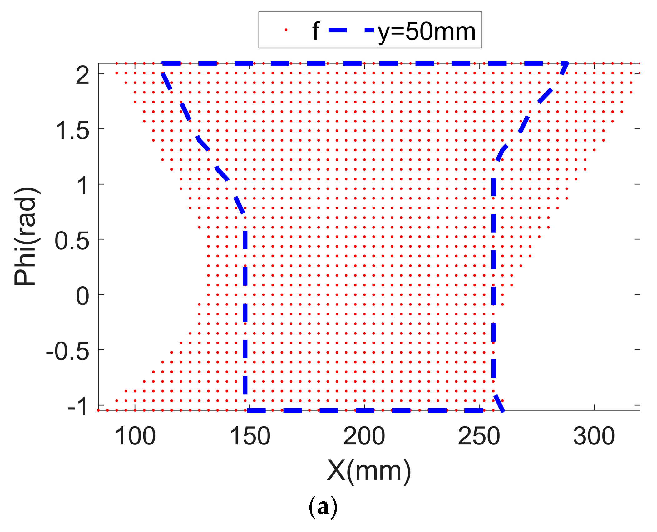
4.1. Workspace Analysis
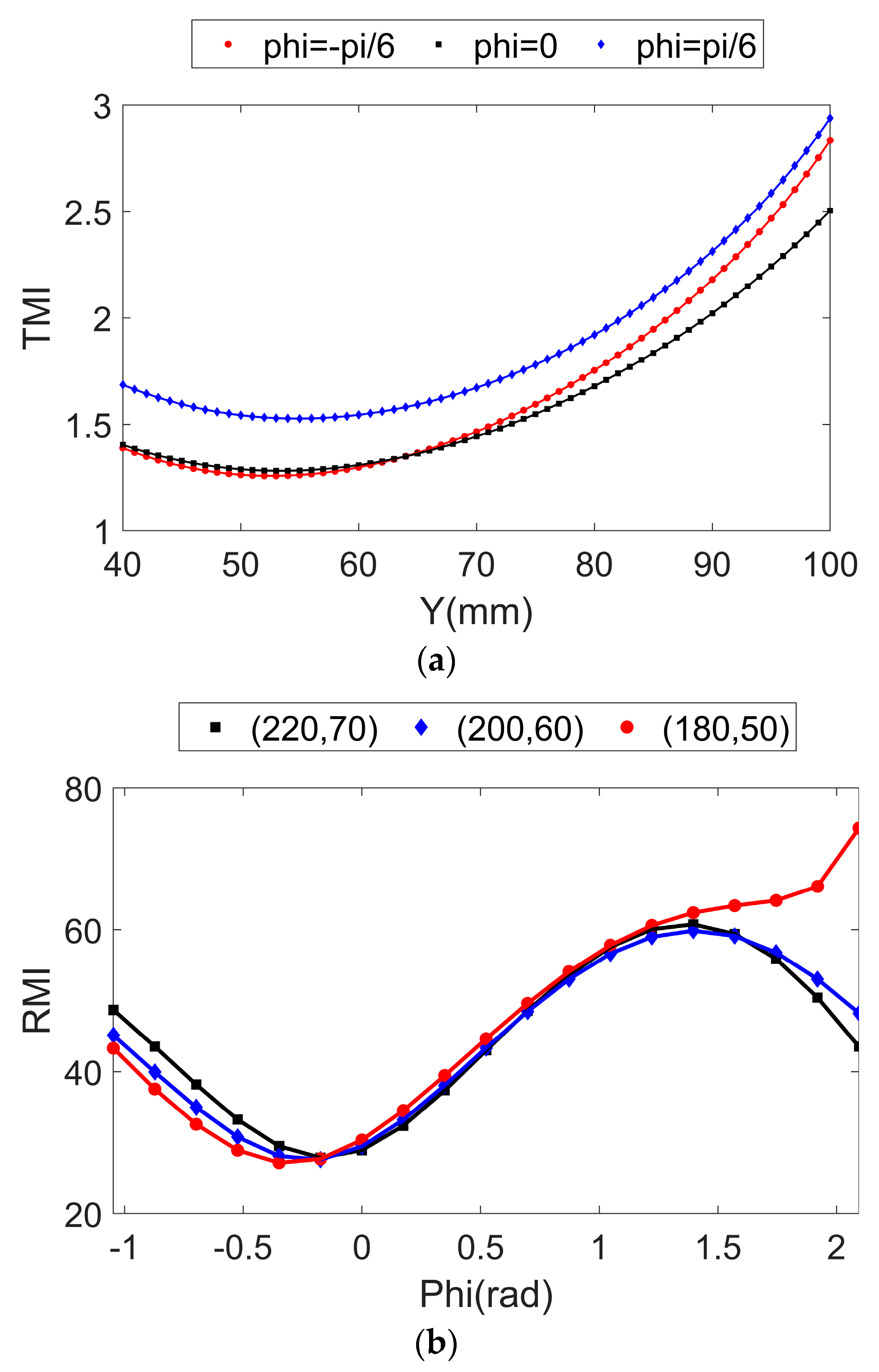
The reachable workspace is one of the most essential indices for a parallel manipulator. For introductive purposes, the linkage dimensions of this parallel manipulator are selected as L1 = 150 mm, L2 = 120 mm, L3 = 20 mm, L4 = 0, L5 = 50 mm, and L6 = 400 mm. The first factor that affects the workspace’s volume is the strokes of the driving joints. In this mechanism, the strokes of three actuation joints are provided as L 3 x 1 , x 2 , x 3 L 6 L 3 . In accordance with the current manipulator configuration in Figure 1b, the ± symbols in Equations (5), (12) and (13) are chosen as , + , and + , respectively. According to the geometric relations, passive angle θ i is computed as
θ 1 = sin 1 [ y 3 L 5 / 3 sin ( φ + π / 6 ) L 4 ] / L 2 θ 2 = sin 1 [ y 3 L 5 / 3 sin ( φ + 5 π / 6 ) L 4 ] / L 2 θ 3 = sin 1 [ y 3 L 5 / 3 sin ( φ + 3 π / 2 ) L 1 + L 4 ] / L 2 .
The driven revolute joints are also constrained as
i π / 2 17 π / 36 θ i i π / 2 π / 36 i = 1 , 2 , 3 π / 3 φ 2 π / 3 .
To solve the reachable workspace, the position range of mobile platform A17B17C17 is predefined as 2 L 3 x L 6 2 L 3 and 2 L 3 y L 1 L 5 . The spatial search methodology is employed to obtain the reachable workspace. The flow diagram of this approach is demonstrated in Figure 3. According to the above conditions, the parameters in this flowchart are listed as xmin = 2L3, xmax = L6 −2L3, xstep = 4 mm, ymin = 2L3, ymax = L1L5, ystep = 1 mm, φ min = π / 3   rad , φ max = 2 π / 3   rad , and φ step = π / 18   rad . In the provided X range, each possible position is employed to compute the corresponding Q based on the inverse kinematic model introduced in Section 3.1. This position will be feasible once it meets all aforementioned constraints.
The reachable workspace of this planar parallel mechanism is computed and shown in Figure 4. Figure 4a–c are the standard views while Figure 4d presents the 3D view. The irregular shape of this workspace can be revealed by the standard views, selected layers, and 3D view. In accordance with Figure 4, when φ = 0 , the workspace is the smallest, and the workspace increases when orientation φ is larger or smaller. The reachable workspace is irregular and asymmetric, which causes difficulty during applications.

4.2. Level Index

There are various kinds of kinematic and dynamic indices that measure the performance of parallel manipulators. They are generally no less than 0 in the entire workspace of the parallel structure. In this section, the novel level index is proposed for evaluating the performance rank of any position/orientation with respect to the overall performance of the workspace. The level index can be computed as follows:
Level   Index = μ ( pose ) μ ¯ + μ ( pose ) ,
where μ ( pose ) is the performance of any pose of the moving platform, and μ ¯ represents the mean value of this kind of performance in the workspace.
Although this level index does not have physical meaning, there are three main advantages of this novel index.
(i) Based on the definition, the level index ranges from 0 to 1, and it is a monotonically increasing function with respect to μ ( pose ) . In other words, if one performance index (it is assumed that larger values denote higher performances) is chosen, the mean level index is constant, and the pose with higher performances will possess a larger level index. The level index can maintain the features of the original index.
We provide the proof here. There are two positions for points a and b. Their corresponding level indices of one specific indicator are LI ( a ) = μ ( a ) / [ μ ¯ + μ ( a ) ] (LI is the abbreviation for the level index) and LI ( b ) = μ ( b ) / [ μ ¯ + μ ( b ) ] , respectively. Parameters μ ( a ) , μ ( b ) , μ ¯ , LI ( a ) , and LI ( b ) are all positive values. Hence, the following expression can be generated.
LI ( b ) LI ( a ) = μ ( b ) μ ¯ + μ ( b ) μ ( a ) μ ¯ + μ ( a ) = μ ( b ) [ μ ¯ + μ ( a ) ] μ ( a ) [ μ ¯ + μ ( b ) ] [ μ ¯ + μ ( a ) ] [ μ ¯ + μ ( b ) ] = μ ¯ [ μ ( b ) μ ( a ) ] [ μ ¯ + μ ( a ) ] [ μ ¯ + μ ( b ) ] .
Equation (29) has an identical positive or negative symbol with respect to μ ( b ) μ ( a ) . Therefore, the level index can retain the original index distributions.
It is noteworthy that the performance index with positive values is suitable for the level index. The performance index with negative numbers can also be arranged (e.g., absolute operation and multiplicative inverse operation) in order to adopt this concept.
(ii) The usage of the level index can also assist in shrinking/normalizing the range of the performance index. For example, the local condition index (LCI) of a parallel mechanism generally ranges from 1 to + . The corresponding level index is limited between 0 and 1. This process will make depictions in figures easier, as the longer axis for the performance index will be replaced.
(iii) The level index provides the performance rating of the parallel mechanism. When comparing two poses from two parallel mechanisms, the same performances with respect to these two poses are not sufficient. Their ratings in the corresponding manipulators are unknown. It is assumed that there are two parallel manipulators with respect to the provided LCI information. Relative to the first parallel manipulator, the mean LCI is 4, and the LCI of point D1 is 5. Relative to the second parallel mechanism, the mean LCI is 10, while the LCI of point D2 is 6. On the one hand, point D1 has a better LCI than that of point D2. On the other hand, the LCI of point D1 is larger than the mean value of the first mechanism. The LCI of point D2 is lower than the mean value of the second mechanism. Considering this aspect, point D1 is worse than point D2. This conclusion can be verified via the local condition level index, which can be deduced using Equation (28). The local condition level indices of these two points are 5/9 and 3/8, respectively, which indicate their ranks in the corresponding mechanisms.
The manipulability index of the mechanism shown in Figure 1b is employed to examine this concept. Taking the derivatives of Equations (4), (10), and (11) with respect to time and rearranging the expression, the following is obtained:
J Q [ x 1 , x 2 , x 3 ] T = J X [ x , y , φ ] T ,
where
J Q = d i a g ( M 1 , M 3 , M 5 )
J X = M 1 M 2 M 1 3 L 5 / 3 sin ( φ + π / 6 ) M 2 3 L 5 / 3 cos ( φ + π / 6 ) M 3 M 4 M 3 3 L 5 / 3 sin ( φ + 5 π / 6 ) M 4 3 L 5 / 3 cos ( φ + 5 π / 6 ) M 5 M 6 M 5 3 L 5 / 3 sin ( φ + 3 π / 2 ) M 6 3 L 5 / 3 cos ( φ + 3 π / 2 )
M 1 = x 3 L 5 / 3 cos ( φ + π / 6 ) x 1
M 2 = y 3 L 5 / 3 sin ( φ + π / 6 ) L 4
M 3 = x 3 L 5 / 3 cos ( φ + 5 π / 6 ) x 2
M 4 = y 3 L 5 / 3 sin ( φ + 5 π / 6 ) L 4
M 5 = x 3 L 5 / 3 cos ( φ + 3 π / 2 ) x 3
M 6 = y 3 L 5 / 3 sin ( φ + 3 π / 2 ) L 1 + L 4 .
Equation (30) can be further expressed as follows:
  Q   = J   X   = ( J Q 1 J X )   X    ,
where J is the Jacobian matrix.
The limitation of   Q .   results in the constraints of   Q .   T   Q .   =   X .   T J T J   X .   . Since term J T J plays a key role in this equation, the manipulability [31] of this planar parallel manipulator can be defined as
M ( J ) = det ( J T J ) .
Since this planar parallel manipulator has translational and rotational movements, it is essential to compute this index separately to avoid the non-homogeneous unit [32]. Equation (31) is divided into the sum of two terms:
  Q   = J V [ x , y ] T + J W [ φ ] T ,
where J V and J W possess, respectively, the first two columns and the last column of Jacobian matrix J.
In accordance with the definition in Equation (32), the translational manipulability index (TMI) and the rotational manipulability index (RMI) are generated as follows:
M ( J V ) = det ( J V T J V ) M ( J W ) = det ( J W T J W ) .
The linkages’ dimensions are already provided in Section 4.1. Both TMI and RMI can be computed and are not associated with position x according to the numerical calculations provided by the software. TMI-y and RMI- φ are plotted in Figure 5. From Figure 5a, TMI decreases at the beginning and then improves as the moving platform moves along the positive Y-axis. The TMI layouts of φ = 0   or   π / 6 are similar. The TMI ranges from 1.24 to 15.4756 in the entire workspace, and the average value is 2.755. Three sets of (x, y) values (unit: mm) are selected to obtain Figure 5b, (180, 50), (200, 60), and (220, 70). From Figure 5b, the RMI distributions of all these scenarios seem cyclic before the first 2/3 period, while the first case indicates an upward trend, and the other two cases maintain this tendency in the following 1/3 period. In the overall workspace, the smallest and largest RMIs are 26.4522 and 244.619, respectively. The mean RMI is 52.7392.
Based on the definition in Equation (28), the manipulability level index (MLI), translational manipulability level index (TMLI), and rotational manipulability level index (RMLI) are formulated as follows:
MLI = M ( J ) M ¯ ( J ) + M ( J ) TMLI = M ( J V ) M ¯ ( J V ) + M ( J V ) RMLI = M ( J W ) M ¯ ( J W ) + M ( J W ) ,
where M ¯ ( J ) , M ¯ ( J V ) , and M ¯ ( J W ) represent the global manipulability index (GMI), global translational manipulability index (GTMI), and global rotational manipulability index (GRMI), respectively. Both analytical and discrete expressions for these indices are denoted as follows:
index ¯ = W ( index ) d W W d W index ¯ = 1 n i = 1 n ( index ) ,
where W denotes the workspace, and n indicates the sum of all sample poses in the workspace.
The corresponding distributions for TMLI and RMLI are depicted in Figure 6, and their trends are exactly the same as those shown in Figure 5. The scales for both TMLI and RMLI are extremely narrow. In the entire workspace, the TMLI ranges from 0.3104 to 0.8489, and the mean value is 0.4703. The RMLI ranges from 0.3340 to 0.8226, and the average value is 0.4853.

5. Dimensional Synthesis

The proper sets of linkage dimensions have significant impacts on the performance distributions and overall characteristics of a parallel mechanism. The employment of linkage optimization is beneficial to search for optimal performances under the pre-described conditions.
Taking into consideration that the hybrid structure serves as a picking-and-placing robot, the reachable workspace volume is one of the most important indicators. TMI and RMI are also beneficial for the selection of parallel mechanism candidates. Hence, three optimization objectives are described as follows:
Objective   1 : 1 Workspace   Volume Objective   2 : 1 GTMI Objective   3 : 1 GRMI ,
where the volume denotes the amount of discrete feasible configurations.
The commonly employed non-dominated sorting genetic algorithm II [33] was chosen in this case. There are 20 individuals in each generation. The maximum generation is set as 60 to guarantee an efficient and global searching process. The ranges of the linkage lengths are provided below (unit: mm).
100 L 1 200 80 L 2 140 10 L 3 40 0 L 4 20 10 L 5 60 100 L 6 500 .
The corresponding constraints of the parallel structure are listed in Section 4.1. After optimization, the trends of the workspace volume, GTMI, and GRMI in each generation are illustrated in Figure 7. As shown in Figure 7, the workspace volume, GTMI, and GRMI exhibit significant increases with respect to generations based on the searched linkage dimensions.
The performances of all individuals in the final generation (Pareto front) are represented in Figure 8. Considering that the workspace is important in picking-and-placing operations, the individual (shown as a blue pentagram in Figure 8) is selected relative to the largest workspace volume. The other individuals are not chosen because the workspace shrinks sharply, although GTMI and GRMI exhibit improvements. The linkage lengths are provided as L1 = 1493.9428 mm, L2 = 114.2580 mm, L3 = 10.0368 mm, L4 = 8.0307 mm, L5 = 12.9197 mm, and L6 = 499.5674 mm. This set of linkages are further rounded as L1 = 150 mm, L2 = 114 mm, L3 = 10 mm, L4 = 8 mm, L5 = 13 mm, and L6 = 500 mm. These three optimization objectives are generated and compared with those of the initial linkages’ lengths (Section 4.1). The corresponding results are shown in Table 1. The corresponding performance ratio is calculated as the ratio between those of the initial linkages and the chosen linkages. From Table 1, the optimized set of linkage has a significantly larger workspace and greater GTMI, with the sacrifice of GRMI.
The reachable workspace of the optimized parallel mechanism is observed in Figure 9. It is evident that the optimized workspace is larger than the initial workspace (Figure 4) in each direction. Compared to the workspace in Figure 4, the improved workspace (Figure 9) is more evenly distributed and is much closer to a regular shape, which ensures that this mechanism is more suitable for industrial applications.
The TMI of the final parallel mechanism can be observed in Figure 10a. Figure 5a and Figure 10a have a similar trend while the latter case has a larger value in each Y-value with respect to a given rotational angle. The RMI of the optimized rods is also illustrated in Figure 10b, which exhibits lower performances than that in Figure 5b for each φ value with a predefined position.

6. Case Study

A simulation is provided to testify the analytical inverse kinematic model and Jacobian matrix. The dimension set in Section 4.1 is employed to construct the three-dimensional prototype in MSC ADAMS [34]. In the initial configuration, the position of the moving platform is (200, 68) mm and φ = 0 . Since this parallel robot enables two translations and one rotation, the displacement of this mobile platform is defined based on the current pose, as listed below:
x = 1 cos ( 1000 t ) 0 0 < t 0.002 π 0.002 π < t 0.009 y = sin ( 1000 t ) 0 0 < t 0.002 π 0.002 π < t 0.009 φ = 0 step ( t , 0.002 π , 0 , 0.008 , π / 50 ) step ( t , 0.008 , π / 50 , 0.0009 , π / 50 ) 0 < t 0.002 π 0.002 π < t 0.008 0.008 < t 0.009 ,
where t indicates the time, and the unit is in seconds. The linear and angular displacement units are mm and rad, respectively.
From Equation (39), the mobile platform travels on a two-dimensional circular path with a constant orientation from 0 to 0.002 π seconds; then, it travels along a smooth curve without translational movements in the remaining period. It is worth noticing that the step function in MSC ADAMS is an approximation step function via the third-degree polynomial.
The positions of three prismatic sliders are measured after the simulation process in MSC ADAMS. The mathematical inverse kinematic model in Section 3.1 is employed to calculate the corresponding analytical positions of these active joints. Figure 11a–c illustrate two sets of results, and the corresponding trajectories of these sliding joints are the same. The positions of the three joints return to their corresponding starting positions during the entire period. The position of the first joint presents an increasing trend from 0 to 0.0027 s and from 0.0058 s to 0.008 s. It decreases from 0.0027 s to 0.0058 s and from 0.008 s to 0.009 s. The position of the second joint decreases from 0 to 0.0005 s and then increases significantly until 0.0036 s. It then exhibits a downward trend until 0.0063 s. The positions are at around 332.4 mm for the rest of this trajectory. The position of the last joint continually increases, with the exception of two other periods: from 0.0027 s to 0.0059 s and from 0.0063 s to 0.008 s.
Furthermore, the linear velocities of these driving joints are measured in MSC ADAMS. The Jacobian matrix expressed in Equation (31) is utilized to compute the analytical velocities of actuators. Both the simulation and analytical results are demonstrated in Figure 11d–f. The two groups of linear velocities match with one another. According to the position trends in Figure 11a–c, the velocities of the first and third joints are similar to two cycles of sine functions while the demarcation point occurs when the time is 0.0062 s; in contrast, the velocities of the second joint possess an additional half cycle of the sine function.
The root mean square errors (RMSEs) of the positions and velocities are derived for quantitative analyses, as listed in Table 2. According to Table 2, the discrepancies of each variable are minute compared with the target trajectory. The obtained velocities of the two methodologies demonstrate higher matching performances than that of positions. The errors come from the rounded values of measurements and computations in the software. The correctness of the analytical inverse kinematic model and the Jacobian matrix is proved using this case. It is worth noticing that the simulation results can outperform some intelligent algorithm-based inverse kinematic models (although the robot structures are not the same). For example, the RMSEs of three deep learning models (multi-layer perceptron, deep LSTM (long short-term memory), and GRU (gated recurrent unit) networks) of the Delta robot are 0.0635, 0.0694, and 0.1009, respectively [35]. The inverse kinematic model employing the optimized neural network of the Stanford robot arm can achieve an RMSE of 9.5588 × 10 4 [36].

7. Discussion

This paper investigated a picking-and-placing hybrid robot based on the planar parallel mechanism. The parallel module provided two translations and one rotation, while belt and rack-and-pinion transmissions enabled extra translation with a large stroke. The actuator for this additional movement is not directly mounted on the moving platform via the unique transmission module, although it exhibits a serial–parallel hybrid structure. The detailed kinematic models for the parallel module and the remaining parts were formulated, which indicated that these two groups of motions are decoupled. More specifically, the translations along the X-axis and Y-axis and the rotation about the Z-axis were determined using the parallel module. The translation along the Z direction was commanded by the belt transmission and rack-and-pinion system.
An approach was proposed to explore the reachable workspace of the parallel manipulator. The novel level index was presented to unify the performance indicator and measure the performance rank in the entire reachable workspace. The manipulability index of the planar parallel architecture was employed to testify to its effectiveness. The dimensional synthesis considering the three targets was provided. In the search process, the workspace volume, GTMI, and GRMI exhibited evident improvements. The detailed performances of the optimal set of linkage dimensions were verified and compared with those of the pre-defined set of linkage lengths. To examine the inverse kinematic solution and the velocity relationship between the actuators and moving platform, a simulation was conducted in MSC ADAMS, and the results matched the analytical solutions.
In future studies, the dynamic characteristics of this proposed 3T1R hybrid robot will be studied, and the level index will be employed for other indices to evaluate industrial robots.

Author Contributions

This work was supervised by D.Z. Under D.Z., Q.Z., D.Z. and G.H. conducted the study together. All authors have read and agreed to the published version of the manuscript.

Funding

This research was funded by the Research Institute for Advanced Manufacturing at the Hong Kong Polytechnic University. The third author would like to acknowledge the financial support provided by the National Natural Science Foundation of China (NSFC) (Grant No. 52305039).

Data Availability Statement

Data sharing is not applicable to this article.

Acknowledgments

The authors would like to thank the financial support from the Research Institute for Advanced Manufacturing at the Hong Kong Polytechnic University. The third author would like to acknowledge the financial support provided by the National Natural Science Foundation of China (NSFC) (Grant No. 52305039).

Conflicts of Interest

The authors declare no conflict of interest.

References

  1. Zheng, S.R.; Park, T.; Hoang, M.C.; Go, G.; Kim, C.S.; Park, J.O.; Choi, E.; Hong, A. Ascidian-inspired soft robots that can crawl, tumble, and pick-and-place objects. IEEE Robot. Autom. Lett. 2021, 6, 1722–1728. [Google Scholar] [CrossRef]
  2. Ghadiri, M.N.; Shavarani, S.M.; Güden, H.; Barenji, R.V. Process sequencing for a pick-and-place robot in a real-life flexible robotic cell. Int. J. Adv. Manuf. Technol. 2019, 103, 3613–3627. [Google Scholar] [CrossRef]
  3. Scalera, L.; Boscariol, P.; Carabin, G.; Vidoni, R.; Gasparetto, A. Enhancing energy efficiency of a 4-DOF parallel robot through task-related analysis. Machines 2020, 8, 10. [Google Scholar] [CrossRef]
  4. Liu, X.J.; Han, G.; Xie, F.G.; Meng, Q.Z. A novel acceleration capacity index based on motion/force transmissibility for high-speed parallel robots. Mech. Mach. Theory 2018, 126, 155–170. [Google Scholar] [CrossRef]
  5. Li, Y.H.; Huang, T.; Chetwynd, D.G. An approach for smooth trajectory planning of high-speed pick-and-place parallel robots using quintic B-splines. Mech. Mach. Theory 2018, 126, 479–490. [Google Scholar] [CrossRef]
  6. Zhao, C.; Wang, K.; Zhao, H.F.; Guo, H.W.; Liu, R.Q. Kinematics, dynamics and experiments of n (3RRlS) reconfigurable series–parallel manipulators for capturing space noncooperative targets. J. Mech. Robot. 2022, 14, 061002. [Google Scholar] [CrossRef]
  7. Clavel, R. Device for the Movement and Positioning of an Element in Space. U.S. Patent 4,976,582, 11 December 1990. [Google Scholar]
  8. Wu, M.K.; Mei, J.P.; Zhao, Y.Q.; Niu, W.T. Vibration reduction of delta robot based on trajectory planning. Mech. Mach. Theory 2020, 153, 104004. [Google Scholar] [CrossRef]
  9. Carabin, G.; Scalera, L.; Wongratanaphisan, T.; Vidoni, R. An energy-efficient approach for 3D printing with a Linear Delta Robot equipped with optimal springs. Robot. Comput. Integr. Manuf. 2021, 67, 102045. [Google Scholar] [CrossRef]
  10. Shen, H.P.; Meng, Q.M.; Li, J.; Deng, J.M.; Wu, G.L. Kinematic sensitivity, parameter identification and calibration of a non-fully symmetric parallel Delta robot. Mech. Mach. Theory 2021, 161, 104311. [Google Scholar] [CrossRef]
  11. Belzile, B.; Eskandary, P.K.; Angeles, J. Workspace determination and feedback control of a pick-and-place parallel robot: Analysis and experiments. IEEE Robot. Autom. Lett. 2019, 5, 40–47. [Google Scholar] [CrossRef]
  12. Staicu, S.; Shao, Z.F.; Zhang, Z.K.; Tang, X.Q.; Wang, L.P. Kinematic analysis of the X4 translational–rotational parallel robot. Int. J. Adv. Robot. Syst. 2018, 15, 1729881418803849. [Google Scholar] [CrossRef]
  13. Mo, J.; Shao, Z.F.; Guan, L.W.; Xie, F.G.; Tang, X.Q. Dynamic performance analysis of the X4 high-speed pick-and-place parallel robot. Robot. Comput. Integr. Manuf. 2017, 46, 48–57. [Google Scholar] [CrossRef]
  14. Han, G.; Xie, F.G.; Liu, X.J. Evaluation of the power consumption of a high-speed parallel robot. Front. Mech. Eng. 2018, 13, 167–178. [Google Scholar] [CrossRef]
  15. Rahul, K.; Raheman, H.; Paradkar, V. Design and development of a 5R 2DOF parallel robot arm for handling paper pot seedlings in a vegetable transplanter. Comput. Electron. Agric. 2019, 166, 105014. [Google Scholar] [CrossRef]
  16. Bourbonnais, F.; Bigras, P.; Bonev, I.A. Minimum-time trajectory planning and control of a pick-and-place five-bar parallel robot. IEEE/ASME Trans. Mechatron. 2014, 20, 740–749. [Google Scholar] [CrossRef]
  17. Nabat, V.; Rodriguez, M.O.; Company, O.; Krut, S.; Pierrot, F. Par4: Very high speed parallel robot for pick-and-place. In Proceedings of the 2005 IEEE/RSJ International Conference on Intelligent Robots and Systems, Edmonton, AB, Canada, 2–6 August 2005; pp. 553–558. [Google Scholar]
  18. Briot, S.; Bonev, I.A. Pantopteron: A new fully decoupled 3DOF translational parallel robot for pick-and-place applications. J. Mech. Robot. 2009, 1, 021001. [Google Scholar] [CrossRef]
  19. Meng, Q.Z.; Xie, F.G.; Liu, X.J. Conceptual design and kinematic analysis of a novel parallel robot for high-speed pick-and-place operations. Front. Mech. Eng. 2018, 13, 211–224. [Google Scholar] [CrossRef]
  20. Huang, T.; Li, Z.X.; Li, M.; Chetwynd, D.G.; Gosselin, C.M. Conceptual design and dimensional synthesis of a novel 2-DOF translational parallel robot for pick-and-place operations. J. Mech. Des. 2004, 126, 449–455. [Google Scholar] [CrossRef]
  21. Huang, T.; Liu, S.T.; Mei, J.P.; Chetwynd, D.G. Optimal design of a 2-DOF pick-and-place parallel robot using dynamic performance indices and angular constraints. Mech. Mach. Theory 2013, 70, 246–253. [Google Scholar] [CrossRef]
  22. Du, X.Q.; Li, Y.C.; Wang, P.C.; Ma, Z.H.; Li, D.W.; Wu, C.Y. Design and optimization of solar tracker with U-PRU-PUS parallel mechanism. Mech. Mach. Theory 2021, 155, 104107. [Google Scholar] [CrossRef]
  23. Chong, Z.H.; Xie, F.G.; Liu, X.J.; Wang, J.S.; Niu, H.F. Design of the parallel mechanism for a hybrid mobile robot in wind turbine blades polishing. Robot. Comput. Integr. Manuf. 2020, 61, 101857. [Google Scholar] [CrossRef]
  24. Li, Y.B.; Wang, L.; Chen, B.; Wang, Z.S.; Sun, P.; Zheng, H.; Xu, T.T.; Qin, S.Y. Optimization of dynamic load distribution of a serial-parallel hybrid humanoid arm. Mech. Mach. Theory 2020, 149, 103792. [Google Scholar] [CrossRef]
  25. Wang, L.P.; Zhang, Z.K.; Shao, Z.F.; Tang, X.Q. Analysis and optimization of a novel planar 5R parallel mechanism with variable actuation modes. Robot. Comput. Integr. Manuf. 2019, 56, 178–190. [Google Scholar] [CrossRef]
  26. Angeles, J. Fundamentals of Robotic Mechanical Systems: Theory, Methods, and Algorithms; Springer: Cham, Switzerland, 2007. [Google Scholar]
  27. Wang, Y.J.; Belzile, B.; Angeles, J.; Li, Q.C. Kinematic analysis and optimum design of a novel 2PUR-2RPU parallel robot. Mech. Mach. Theory 2019, 139, 407–423. [Google Scholar] [CrossRef]
  28. Patel, S.; Sobh, T. Manipulator performance measures-a comprehensive literature survey. J. Intell. Robot. Syst. 2015, 77, 547–570. [Google Scholar] [CrossRef]
  29. Brinker, J.; Corves, B.; Takeda, Y. Kinematic performance evaluation of high-speed Delta parallel robots based on motion/force transmission indices. Mech. Mach. Theory 2018, 125, 111–125. [Google Scholar] [CrossRef]
  30. Zou, Q. Type Synthesis and Performance Optimization of Parallel Manipulators. Ph.D. Dissertation, York University, Toronto, ON, Canada, 2022. [Google Scholar]
  31. Cardou, P.; Bouchard, S.; Gosselin, C. Kinematic-sensitivity indices for dimensionally nonhomogeneous Jacobian matrices. IEEE Trans. Robot. 2010, 26, 166–173. [Google Scholar] [CrossRef]
  32. Khan, S.; Andersson, K.; Wikander, J. Jacobian matrix normalization—A comparison of different approaches in the context of multi-objective optimization of 6-DOF haptic devices. J. Intell. Robot. 2015, 79, 87–100. [Google Scholar] [CrossRef]
  33. Shentu, S.Z.; Xie, F.G.; Liu, X.J.; Gong, Z. Motion control and trajectory planning for obstacle avoidance of the mobile parallel robot driven by three tracked vehicles. Robotica 2021, 39, 1037–1050. [Google Scholar] [CrossRef]
  34. Niu, J.Y.; Wang, H.B.; Shi, H.M.; Pop, N.; Li, D.; Li, S.S.; Wu, S.Z. Study on structural modeling and kinematics analysis of a novel wheel-legged rescue robot. Int. J. Adv. Robot. Syst. 2018, 15, 1729881417752758. [Google Scholar] [CrossRef]
  35. Toquica, J.S.; Oliveira, P.S.; Souza, W.S.R.; Motta, J.M.S.T.; Borges, D.L. An analytical and a Deep Learning model for solving the inverse kinematic problem of an industrial parallel robot. Comput. Ind. Eng. 2021, 151, 106682. [Google Scholar] [CrossRef]
  36. KöKer, R. A genetic algorithm approach to a neural-network-based inverse kinematics solution of robotic manipulators based on error minimization. Inf. Sci. 2013, 222, 528–543. [Google Scholar] [CrossRef]
Figure 1. Schematic diagram of the industrial robot. (a) The 4-DOF hybrid manipulator; (b) the planar parallel mechanism.
Machines 11 00979 g001aMachines 11 00979 g001b
Figure 2. Initial configuration of the Z-translation system.
Machines 11 00979 g002
Figure 3. Flow diagram for the reachable workspace.
Machines 11 00979 g003
Figure 4. Reachable workspace and specific layers (f, s, and t, respectively, represent front, side, and top views): (a) front view; (b) side view; (c) top view; (d) 3D view.
Machines 11 00979 g004aMachines 11 00979 g004b
Figure 5. Distributions of two manipulability indices: (a) translational manipulability index under constant orientations; (b) rotational manipulability index under constant positions.
Machines 11 00979 g005
Figure 6. Layouts of two manipulability level indices: (a) translational manipulability level index under fixed orientations; (b) rotational manipulability level index under fixed positions.
Machines 11 00979 g006aMachines 11 00979 g006b
Figure 7. Performances in the optimization process: (a) workspace volume; (b) GTMI and GRMI.
Machines 11 00979 g007
Figure 8. The performance of the last generation (the blue pentagram is the selected performance).
Machines 11 00979 g008
Figure 9. Diagrams for reachable workspace and layers (f, s, and t, respectively, denote front, side, and top views): (a) front view; (b) side view; (c) top view; (d) 3D view.
Machines 11 00979 g009aMachines 11 00979 g009b
Figure 10. Performance layouts of the optimized parallel structure: (a) translational manipulability index under constant orientations; (b) rotational manipulability index under constant positions.
Machines 11 00979 g010
Figure 11. Comparison between the analytic and simulation results (A—analytics; S—simulation): (a) position of the first slider; (b) position of the second slider; (c) position of the third slider; (d) velocity of the first slider; (e) velocity of the second slider; (f) velocity of the third slider.
Machines 11 00979 g011aMachines 11 00979 g011bMachines 11 00979 g011c
Table 1. Performance comparisons between two sets of linkages.
Workspace VolumeGTMIGRMI
Initial linkages71,4282.755052.7392
Optimized linkages124,7453.232714.5590
Performance ratio174.64%117.34%27.61%
Table 2. RMSEs of two approaches.
MotorFirst MotorSecond MotorThird Motor
RMSE of position 1.03 × 10 4 8.973 × 10 4 5.862 × 10 4
RMSE of velocity 1.342 × 10 4 1.555 × 10 4 1.805 × 10 4
Disclaimer/Publisher’s Note: The statements, opinions and data contained in all publications are solely those of the individual author(s) and contributor(s) and not of MDPI and/or the editor(s). MDPI and/or the editor(s) disclaim responsibility for any injury to people or property resulting from any ideas, methods, instructions or products referred to in the content.

