Article

Synchronization Control for a Mobile Manipulator Robot (MMR) System: A First Approach Using Trajectory Tracking Master–Slave Configuration

by
Jorge Gustavo Pérez-Fuentevilla
1,
América Berenice Morales-Díaz
2,*,† and
Alejandro Rodríguez-Ángeles
1,†
1
Departamento de Ingeniería Eléctrica, CINVESTAV-IPN, Mexico City 07360, Mexico
2
Robótica y Manufactura Avanzada, CINVESTAV-Saltillo, Ramos Arizpe 25900, Mexico
*
Author to whom correspondence should be addressed.
These authors contributed equally to this work.
Machines 2023, 11(10), 962; https://doi.org/10.3390/machines11100962
Submission received: 12 July 2023 / Revised: 7 September 2023 / Accepted: 7 September 2023 / Published: 16 October 2023
(This article belongs to the Special Issue Advanced Motion Control of Multiple Robots)

Abstract

:
In cooperative tasks, the ability to keep a kinematic relationship between the robots involved is essential. The main goal in this work is to design a synchronization control law for mobile manipulator robots (MMRs) considering a (2,0) differential mobile platform, which possesses a non-holonomic motion constraint. To fulfill this purpose, a generalized trajectory tracking control law based on the computed torque technique, for an MMR with n degrees of freedom, is presented. Using Lyapunov stability theory, it is shown that the closed loop system is semiglobal and uniformly ultimately boundedness (UUB) stable. To add position-level static coupling terms to achieve synchronization on a group of MMRs, the control law designed for the trajectory tracking problem is extended. Both experimental and numerical simulation results are presented to show the designed controllers performance. A successful experimental validation for the trajectory tracking problem using an 8 degrees of freedom (DoF) robot model (KUKA youBot) is depicted. Finally, numerical simulations in the CoppeliaSim environment are shown, which are used to test the synchronization control law made on the hypothetical scenario, where a two robot system has to manipulate an object over a parametric trajectory.

1. Introduction

Entrusting a single robot to deal with complex or heavy tasks may not be the best option: some tasks require more than one robot, so in that sense, the synchronization of multi-robot systems represents a better solution. For this reason, it has been an intensive area of research in the last decades. Cooperative manipulation is one of the methods used to deal with the synchronization idea; it allows a multi-robot system to manipulate a heavy and/or big object more efficiently than a single robot.
There are some classical approaches to achieve coordination on a robot system [1]: one of them is the master–slave strategy, which is used in this work. In this strategy, a master MMR is considered, which is in charge of setting up the trajectory reference for the slave MMRs while using cross-coupled controls to synchronize motions amongst the robots; therefore, a kinematic relationship can be maintained for a desired task.
There are some interesting approaches for synchronizing fixed-base manipulators, for example, synchronization control based on output differential flatness [2]; in [3], the robustness of the sliding mode technique is considered; in [4], a system under parametric uncertainties is considered; in [5], the authors deal with dynamical uncertainties; and in [6], the problem of obstacle avoidance is solved. More recently, sophisticated controllers have been considered, see, for instance, [7], where a non-linear model predictive control is used for the synchronization problem at position and force levels.
Mobile robots are also a case of study on synchronization. In [1], a swarm of mobile robots that can switch between formations are presented; in [8], a discrete approach on differential robots is developed; also, varying formations have been considered; this is the case in [9].
For the case of control MMRs, there are some works reported for the trajectory tracking control; in [10], the authors solved the trajectory tracking problem by designing a robust controller based-on sliding mode technique; an extended state observer and movement constraint in the mobile base was introduced in [11]; and another approach was taken in [12], where the dynamical model of MMR is obtained by using Gibbs–Appell formulation instead of the classical Lagrange methodology. However, these works do not consider the synchronization approach.
The present work has the goal of synchronizing MMRs; to this end, a position-level synchronization control law using a master–slave scheme with cross-coupled terms is provided as an immediate extension of a trajectory tracking controller. The trajectory tracking problem for a n DoF MMR is solved designing a non-linear control law based-on a computed torque control with gravity compensation.
This work is organized as follows. In Section 2, the dynamic equations of the n DoF MMR are developed. In Section 3, the controller design and stability analysis are addressed. The master–slave synchronization is posted as an extension of the trajectory tracking controller in Section 4. The results are depicted in Section 5, and the findings and conclusions are summarized in Section 2.

2. Problem Statement

Consider the n DoF MMR configuration shown in Figure 1, where {0} frame corresponds to inertial frame, and the end-effector frame is denoted by {e}.
Let us define n = n b + n m , where n b = 3 is the number of DoF for the mobile base and n m corresponds to the number of DoF for the manipulator. This way, generalized coordinates are defined as q b = x y θ for the mobile and q m = ϕ 1 ϕ 2 ϕ n m for the manipulator. This yields q ( t ) = q b q m for the whole system, namely,
q ( t ) = q 1 q 2 q n = x y θ ϕ 1 ϕ 2 ϕ n m .
where ( x , y , θ ) is the Cartesian position and orientation of the mobile base on the ( x 0 , y 0 ) plane and ϕ i , i = 1 , , n m are the angular positions for the i-th link.
A (2, 0) type differential mobile robot is considered, meaning that the MMR platform is governed by the kinematic model shown in (2) for the mobile part.
x ˙ = v cos θ y ˙ = v sin θ θ ˙ = ω .
where ( x ˙ , y ˙ ) are the Cartesian velocities, θ ˙ is its angular velocity on the ( x 0 , y 0 ) plane, and v is the longitudinal velocity. From (2), it is easy to obtain the non-holonomic constraint that the mobile robot satisfies as
x ˙ sin θ y ˙ cos θ = 0 .

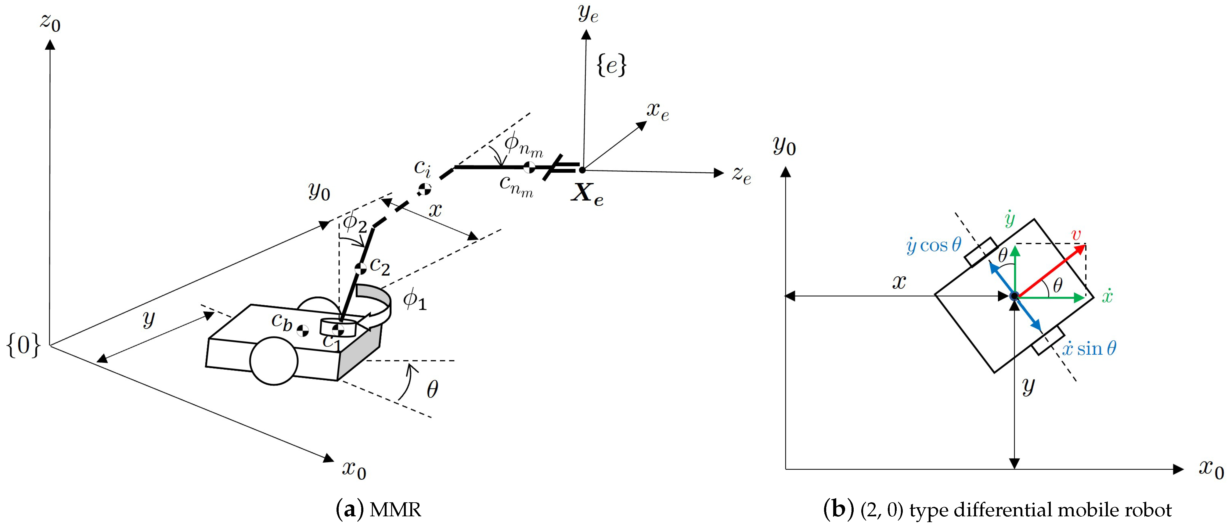
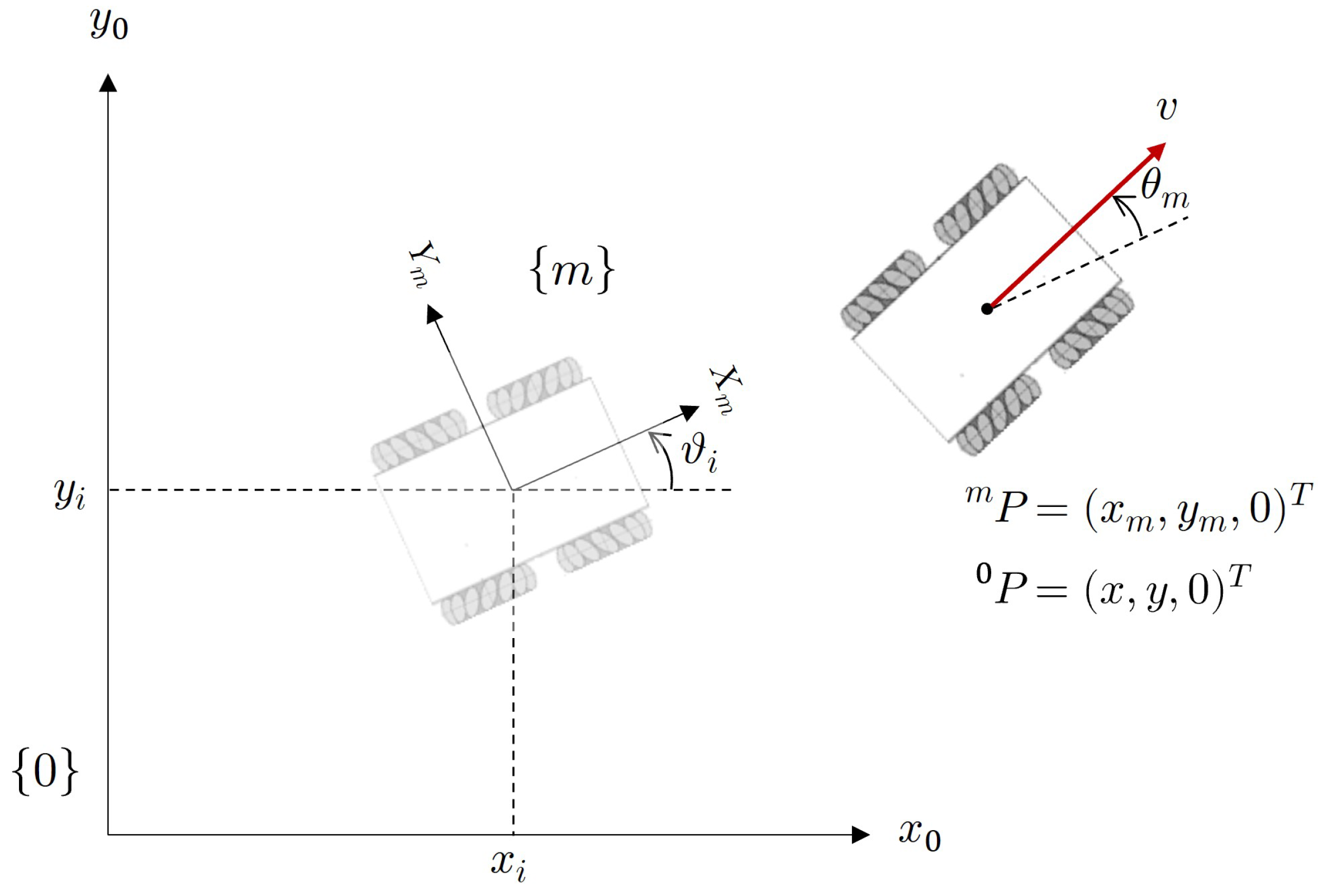
2.1. Forward and Inverse Kinematics

The deal with forward kinematics is being able to describe the pose of the end-effector X e as a function of q ( t ) , i.e.,
X e = 0 P e 0 O e = f ( q ) ,
where 0 P e is the position vector of the end-effector measured from inertial frame {0} and 0 O e describes its orientation. X e R ρ is defined on the task-space.
On the other hand, inverse kinematics is about finding solutions for q ( t ) given a pose vector X e , i.e.,
q ( t ) = f 1 ( X e ) .
For redundant robots, such as the MMRs considered, solving the inverse kinematics is a complicated task since the number of DoF is greater than the task-space dimension, i.e., n > ρ . This implies having multiple solutions for q ( t ) given a desired trajectory, which could be a problem because some discontinuities could appear from one solution to another, but it is also advantageous since the robot can satisfy a task in more than one way.

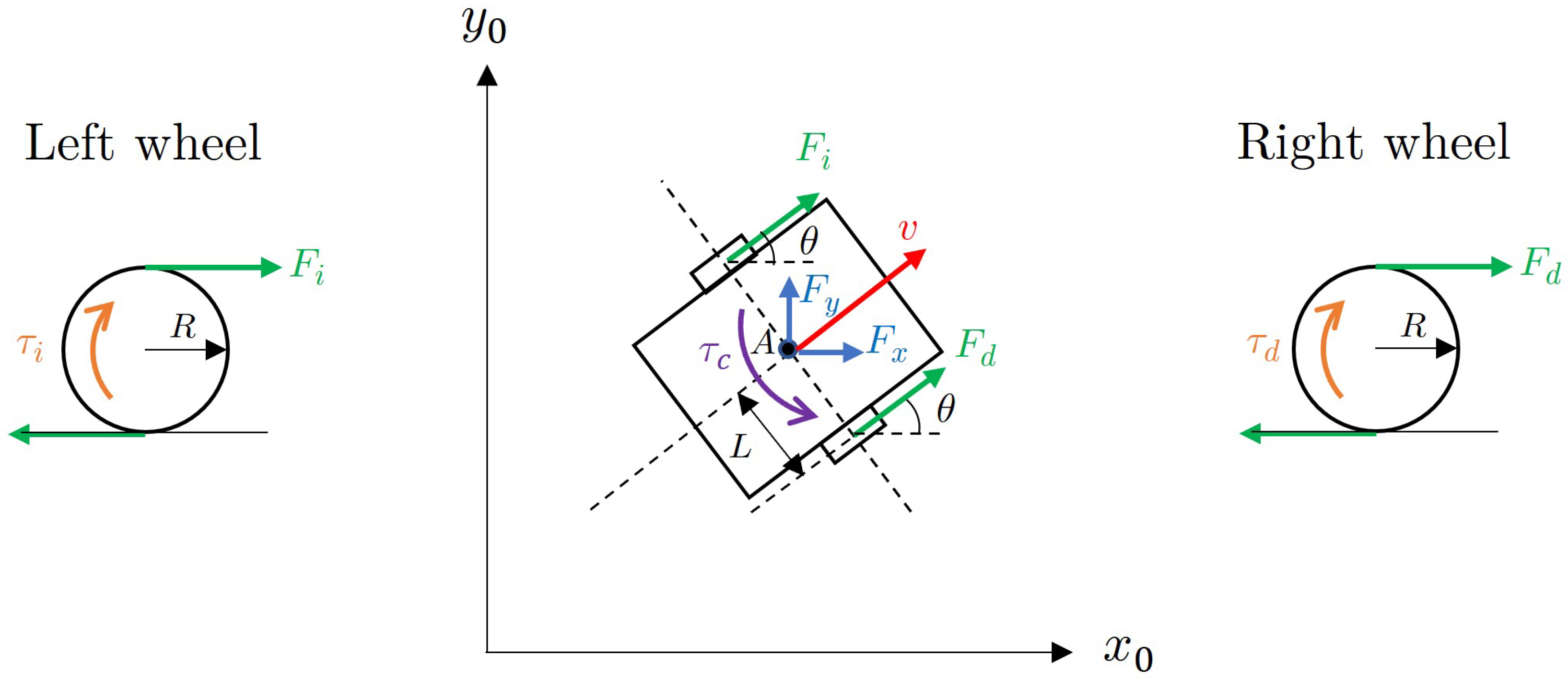
2.2. Generalized Dynamical Model

For a robot without kinematic constraints, the dynamical model can be described as
D ( q ) q ¨ + C ( q , q ˙ ) q ˙ + F f ( q , q ˙ ) + G ( q ) = τ J e ( q ) h r .
where D ( q ) R n × n is the inertia matrix; C ( q , q ˙ ) q ˙ R n × n is the Coriolis matrix; F f ( q , q ˙ ) R n is the force vector due to friction; G ( q ) R n is the gravitational effects vector; J e ( q ) R ρ × n is the Jacobian matrix that relates the articular velocities with the end-effector velocities ( X ˙ e = J e ( q ) q ˙ ); h r R ρ is the generalized forces vector due to robot interaction with the environment, if there is no interaction with the environment J e ( q ) h r = 0 ; τ = F x F y τ c τ 1 τ 2 τ n m R n is the control forces vector; F x and F y are the translation forces on the x 0 and y 0 axis, respectively; τ c is the mobile torque with respect to its rotation axis; and τ i , i = 1 , 2 , , n m is the torque of the i-th link. All the torques and forces on the mobile platform are shown in Figure 2.
The problem with model (6) is that the non-holonomic constraint (3) is not satisfied. The incorporation of the constraint into the dynamical model is achieved through the next procedure, [13,14].
The non-holonomic constraint (3) can be re-written as A ( q ) q ˙ = 0 , with A ( q ) R k × n being k = 1 the number of independent constraints; this yields
A ( q ) = sin θ cos θ 0 0 1 × n m ,
where 0 1 × n m is a row vector of n m zeros.
Let S ( q ) R n × ( n k ) be an invertible full-rank matrix that spans the null space of A ( q ) , i.e., S ( q ) A ( q ) = 0 is satisfied (or equivalently, A ( q ) S ( q ) = 0 ). Thus,
S ( q ) = cos θ 0 0 1 × n m sin θ 0 0 1 × n m 0 1 0 1 × n m 0 n m × 1 0 n m × 1 1 n m × n m ,
with 0 n m × 1 a column vector of n m zeros and 1 n m × n m the identity matrix of dimension n m × n m .
An auxiliary vector η ( t ) R n k exists that satisfies
q ˙ ( t ) = S ( q ) η ( t ) ,
which is defined as
η ( t ) = η 1 η 2 η n 1 = v θ ˙ ϕ ˙ 1 ϕ ˙ 2 ϕ ˙ n m .
Let τ i and τ d be the left and right wheels torque, respectively, see Figure 2. It is possible to write τ = B ( q ) τ r e d with B ( q ) R n × ( n k ) , where:
τ r e d = τ d τ i τ 1 τ 2 τ n m
B ( q ) = 1 R cos θ 1 R cos θ 0 1 × n m 1 R sin θ 1 R sin θ 0 1 × n m L R L R 0 1 × n m 0 n m × 1 0 n m × 1 1 n m × n m .
With R being the radius of the wheels and L the length from the longitudinal axis of the mobile robot to the wheels.
Finally, the constrained model is defined as follows:
D ¯ ( q ) η ˙ + C ¯ ( q , q ˙ ) η + F ¯ f ( q , q ˙ ) + G ¯ ( q ) = τ ¯ ( q ) q ˙ = S ( q ) η .
where:
D ¯ ( q ) = S ( q ) D ( q ) S ( q ) R ( n k ) × ( n k ) C ¯ ( q , q ˙ ) = S ( q ) D ( q ) S ˙ ( q ) + S ( q ) C ( q , q ˙ ) S ( q ) R ( n k ) × ( n k ) F ¯ f ( q , q ˙ ) = S ( q ) F f ( q , q ˙ ) R n k G ¯ ( q ) = S ( q ) G ( q ) R n k τ ¯ ( q ) = S ( q ) B ( q ) τ r e d S ( q ) J e ( q ) h r R n k .
B ( q ) is called the motorization matrix, and it establishes the relationship between the generalized forces vector τ of the unconstrained model (6) and a new control vector τ r e d used for the new model (13), where the non-holonomic constraint is satisfied. Notice that the kinematic model (2) is inside the relationship (9); therefore, model (13) satisfies the mobile constraint in a natural way.

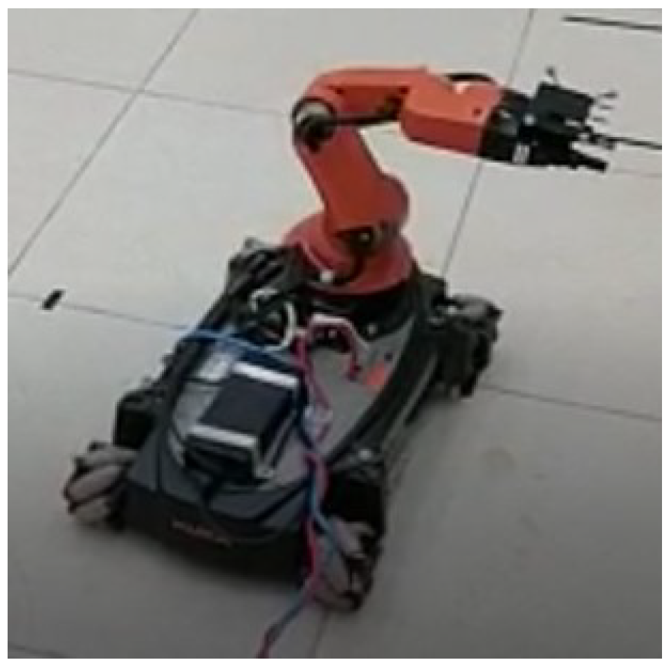
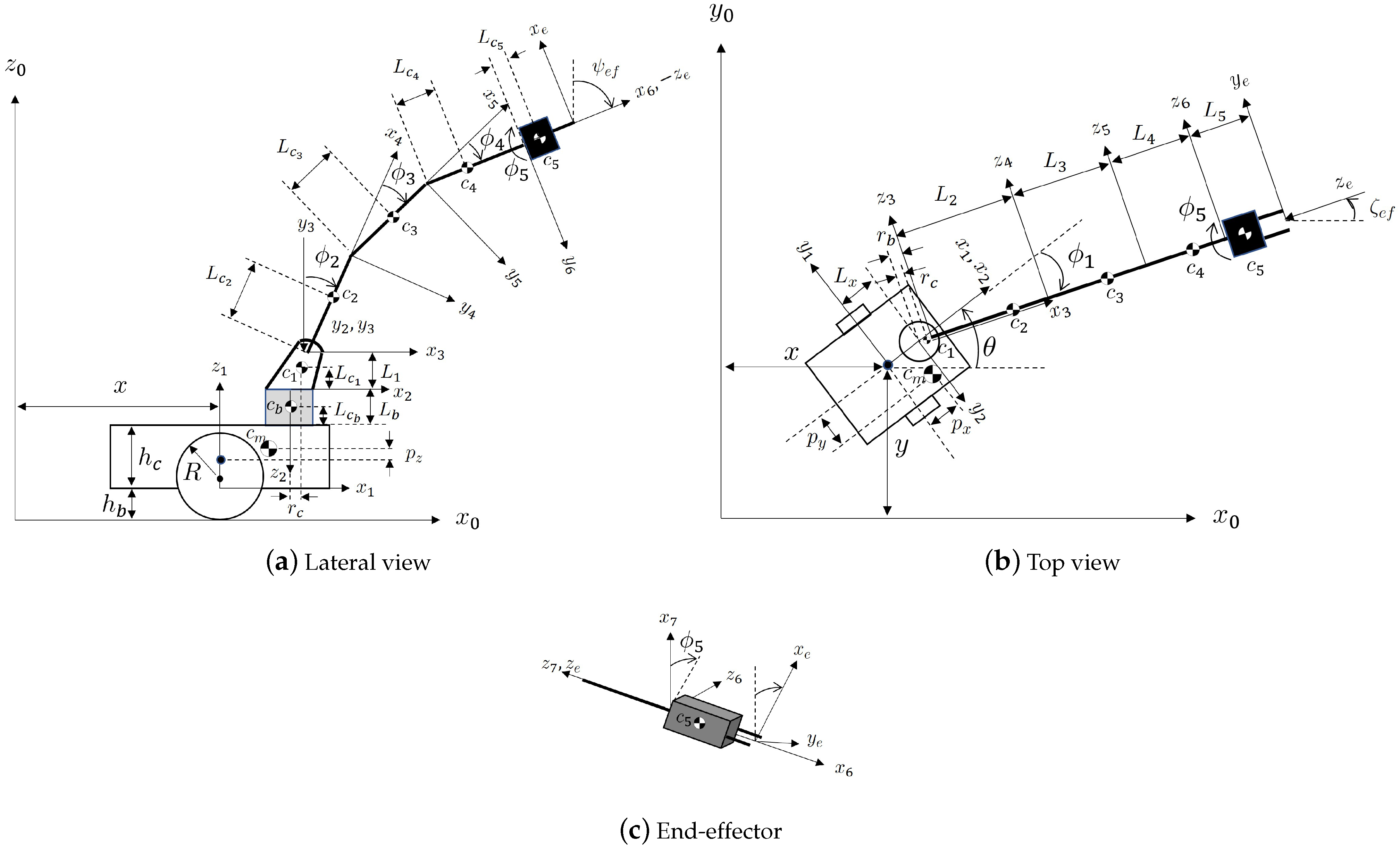
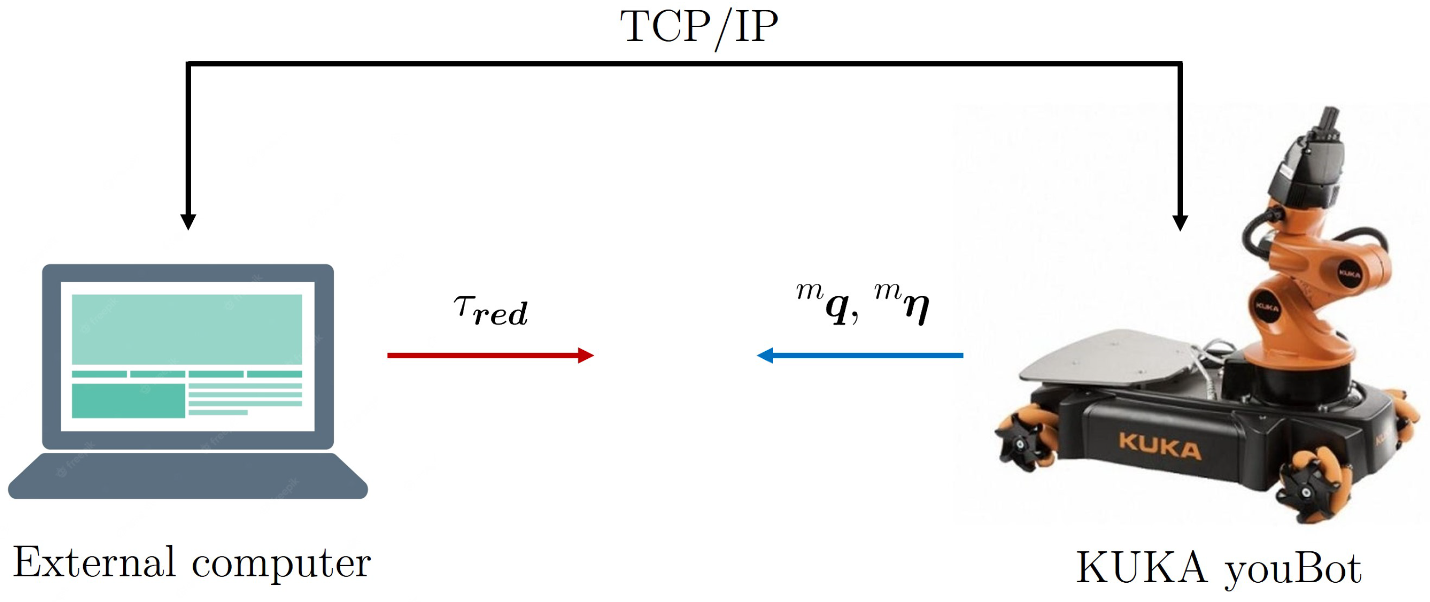
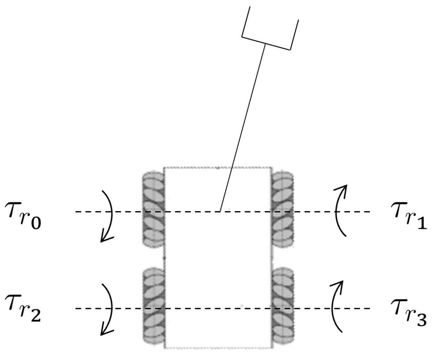
2.3. Particular Case: KUKA youBot

The KUKA youBot is an 8 DoF industrial-type MMR ( n = 8 ) that is also used for research purposes [15]. It is composed of a 5 DoF arm mounted on a omnidirectional mobile base, considered as a differential mobile base in this work by constraining the wheels of each side of the platform so they move at the same velocity. See Figure 3.
KUKA youBot wheels are of the Mecanum type; these kind of wheels are composed of a series of rollers placed at 45 degrees from the rotation axis and allow for longitudinal and transversal motion; however, when the two wheels of each side rotate at the same angular speed and direction, the transversal velocity is zero, and the omnidirectional base can only have longitudinal and angular velocities (see the kinematic model for an omnidirectional platfom in [16]).
The following assumptions for the mobile base are considered:
  • The two wheels of each side rotate at the same speed.
  • The robot is running on a firm ground surface.
  • The four wheels are always in contact with the ground surface.
  • There is no slippage between the wheels and the ground surface.
With these considerations, and the fact that the moving direction of KUKA youBot wheels is the mobile longitudinal axis, i.e., it has not orientation movement, the KUKA youBot mobile base can be treated as a (2, 0) type differential mobile base [17].
The MMR configuration is depicted in Figure 4.
Consider the symmetrical elements (mobile base and links) in the KUKA configuration, and the inertia tensor matrix of each element is defined as i I i = diag I i x x I i y y I i z z , i = m , b , 1 , , 5 measured in local frame; then, the parameters are defined as follows:
  • c m , c b , c i , i = 1 , , 5 : Mobile base, fixed link, and i-th link center of mass (CoM).
  • m m , m b , m i , i = 1 , , 5 : Mobile base, fixed link, and i-th link mass.
  • h b , h c : Distance from the floor to mobile base, and mobile base height, respectively.
  • R: Wheels radius.
  • p x , p y , p z : Distances to the mobile base CoM.
  • L: Distance measured from mobile base longitudinal axis to its wheels.
  • L i , i = b , 1 , , 5 : i-th link length.
  • L c i , i = b , 1 , , 5 : Length to the i-th link CoM.
  • r b , r c : Radius measured on the ( x 0 , y 0 ) plane, from the fixed link CoM to the second link base, and to the first link CoM, respectively.
  • L x : Distance measured on the ( x 0 , y 0 ) plane, from the mobile base centroid to the fixed link centroid.
  • i I i , i = m , b , 1 , , 5 : i-th element inertia tensor.
  • b q i , i = 1 , , 8 : viscous friction coefficient related to the generalized coordinate q i .

2.3.1. Forward Kinematics

Let us define 0 P e = x e f y e f z e f as the position vector for the end-effector on the inertial frame, and 0 O e = ψ e f ζ e f for the orientation, where ψ e f is the end-effector orientation with respect to the vertical axis ( z 0 ) and ζ e f is the end-effector orientation with respect to the horizontal axis ( x 0 ); the third orientation for the end-effector would be directly affected by ϕ 5 , namely, the wrist rotation; however, for the task contemplated in this work this is not necessary, and it is not taken into account. The above considerations allow one to define the end-effector pose as follows:
X e = x e f y e f z e f ψ e f ζ e f .
The end-effector is related to the inertial frame {0} through the homogeneous matrix defined as:
0 T e = 0 R e 0 P e 0 1 × 3 1 .
where:
0 R e = sin ϕ 1 θ sin ϕ 5 cos ϕ 1 θ α 1 cos ϕ 5 sin ϕ 1 θ cos ϕ 5 + α 1 cos ϕ 1 θ sin ϕ 5 α 2 cos ϕ 1 θ cos ϕ 1 θ sin ϕ 5 + α 1 sin ϕ 1 θ cos ϕ 5 cos ϕ 1 θ cos ϕ 5 α 1 sin ϕ 1 θ sin ϕ 5 α 2 sin ϕ 1 θ α 2 cos ϕ 5 α 2 sin ϕ 5 α 1
0 P e = x + L x cos θ + r b + L 2 sin ϕ 2 + L 3 sin ϕ 2 + ϕ 3 + L 4 + L 5 sin ϕ 2 + ϕ 3 + ϕ 4 cos ϕ 1 θ y + L x sin θ r b + L 2 sin ϕ 2 + L 3 sin ϕ 2 + ϕ 3 + L 4 + L 5 sin ϕ 2 + ϕ 3 + ϕ 4 sin ϕ 1 θ h b + h c + L 1 + L b + L 2 cos ϕ 2 + L 3 cos ϕ 2 + ϕ 3 + L 4 + L 5 cos ϕ 2 + ϕ 3 + ϕ 4 α 1 = cos ϕ 2 + ϕ 3 + ϕ 4 , α 2 = sin ϕ 2 + ϕ 3 + ϕ 4 .
0 R e R 3 × 3 is the rotation matrix (another representation for orientation) and 0 1 × 3 = 0 0 0 .

2.3.2. Inverse Kinematics

From Figure 4, it is easy to see that orientations in (14) are defined as follows:
ζ e f = θ ϕ 1
ψ e f = ϕ 2 + ϕ 3 + ϕ 4 .
where θ can be written in terms of mobile cartesian velocities —computing θ could be tricky due to the tan 1 function. In order to avoid quadrant problems and inconsistencies (such as having x ˙ = 0 ), it is recomended to use atan 2 , function instead—, i.e.,
θ = tan 1 y ˙ x ˙ .
A simple way for solving the inverse kinematics is defining a desired pose vector X ed = x e f d y e f d z e f d ψ e f d ζ e f d for the end-effector and a desired cartesian position for the mobile base x d y d . This way, θ can be obtained in desired velocities terms and the desired orientation ζ e f d can be used to obtain ϕ 1 in (18). Setting (17) equal to the end-effector desired position x e f d y e f d z e f d and using the desired orientation ψ e f d in (19), we obtain a system of non-linear equations that are numerically solved for ϕ 2 , ϕ 3 and ϕ 4 .
Finally, note that ϕ 5 does not affect the end-effector position nor orientation ( ϕ 5 is used for rotating the wrist). We can simply establish ϕ 5 as a constant.

2.3.3. Dynamical Model

The dynamical model is such that n = 8 ( n b = 3 and n m = 5 ). The detailed definitions of the KUKA youBot model can be found in [18].

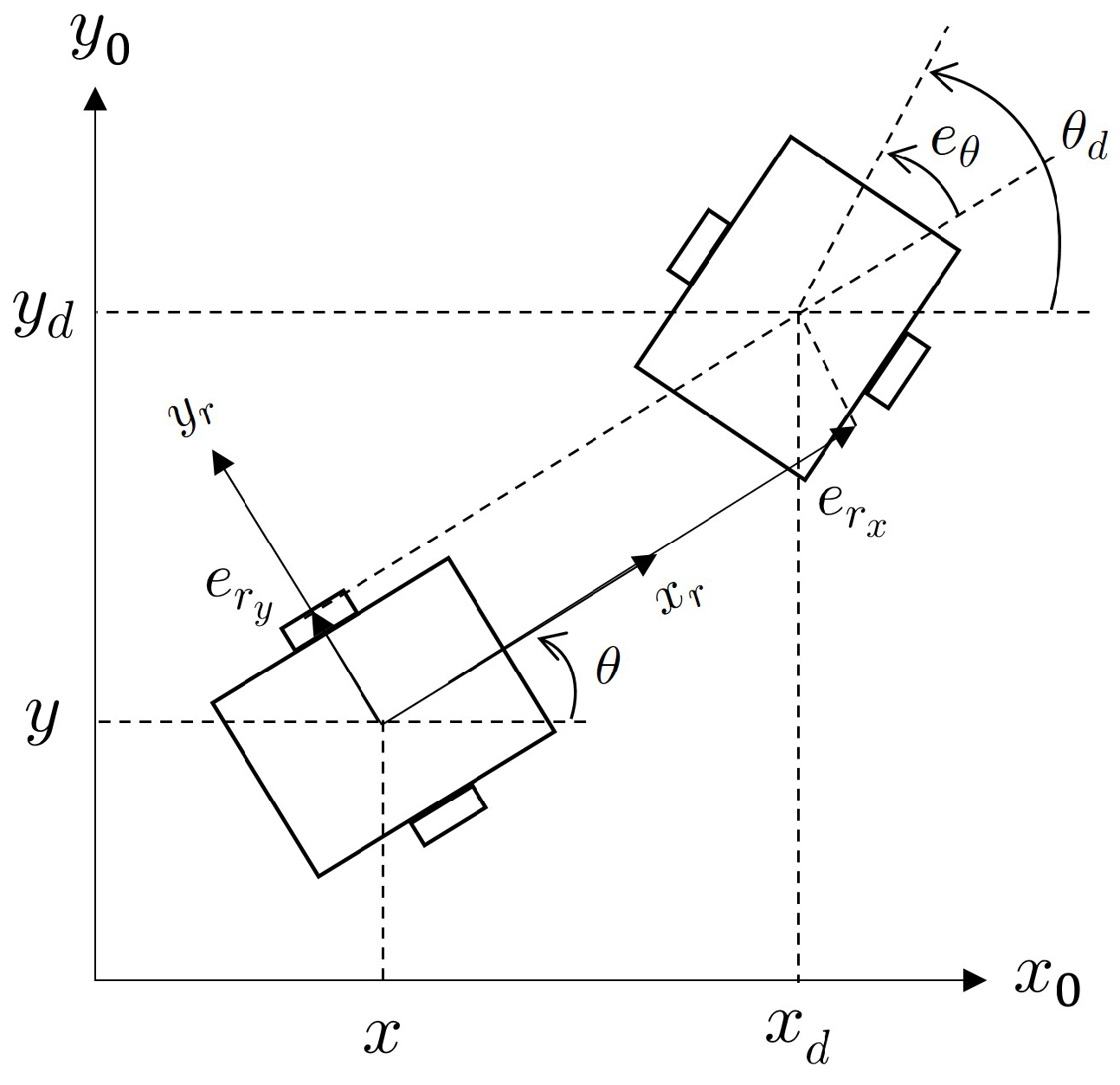
3. Trajectory Tracking Problem

Let q d ( t ) and η d ( t ) be the desired position and velocity vectors, namely,
q d ( t ) = q 1 d q 2 d q n d = x d y d θ d ϕ 1 d ϕ n m d
η d ( t ) = S ( q d ) q ˙ d = η 1 d η 2 d η ( n 1 ) d = v d θ ˙ d ϕ ˙ 1 d ϕ ˙ n m d ,
to satisfy the non-holonomic constraint, in terms of desired values, we obtain
θ d = tan 1 y ˙ d x ˙ d ,
the mobile velocity references are:
v d = x ˙ d 2 + y ˙ d 2 , θ ˙ d = x ˙ d y ¨ d x ¨ d y ˙ d v d 2 .
The desired trajectories are designed to be smooth functions, i.e., at least twice differentiable and considering that v d 0 .
Let us define the position and velocity error vectors:
e q = q d q = e x e y e θ e ϕ 1 e ϕ n m
e η = η d η = e v e ˙ θ e ˙ ϕ 1 e ˙ ϕ n m .
For a differential robot, the trajectory tracking problem can be solved by using a leader-follower scheme, where the leader is proposed to be a virtual robot, and it describes, ideally, the desired trajectory. The objective is that the actual robot converges with the virtual robot [19]. This is represented in Figure 5.
The trajectory tracking error vector, in the actual robot local frame, with respect to the virtual robot, is defined as follows:
e r = e r x e r y e θ = cos θ sin θ 0 sin θ cos θ 0 0 0 1 x d x y d y θ d θ .
For an MMR with no interaction with the environment, the generalized trajectory tracking control law is proposed as:
τ red = P 1 ( q ) H ( q ) I 1 ( q , η ) + η ˙ d + K p e η + U ( q , q d , η d ) + G * ( q ) + F f * ( q , q ˙ ) R n 1 .
where:
U ( q , q d , η d ) = u 1 u 2 u n 1 u 1 = k 1 e r x u 2 = k 2 v d sin e θ e θ e r y + k 3 e θ u 3 = k 4 e ϕ 1 u n 1 = k n e ϕ n m
P q = S q B q , H q = D ¯ q , I 1 q , η = D ¯ 1 q C ¯ q , q ˙ η G * q = D ¯ 1 q G ¯ q , F f * ( q , q ˙ ) = D ¯ 1 q F ¯ f q , q ˙ .
With gains:
k i > 0 , i = 1 , , n .
K p = diag { k p 1 k p 2 k p n 1 } > 0 R ( n 1 ) × ( n 1 ) is a diagonal positive definite matrix, U ( q , q d , η d ) is the vector in charge of correcting the position error, G * q is the gravity compensation term, and F f * ( q , q ˙ ) compensates friction effects.
The block diagram of the controlled system is shown in Figure 6.

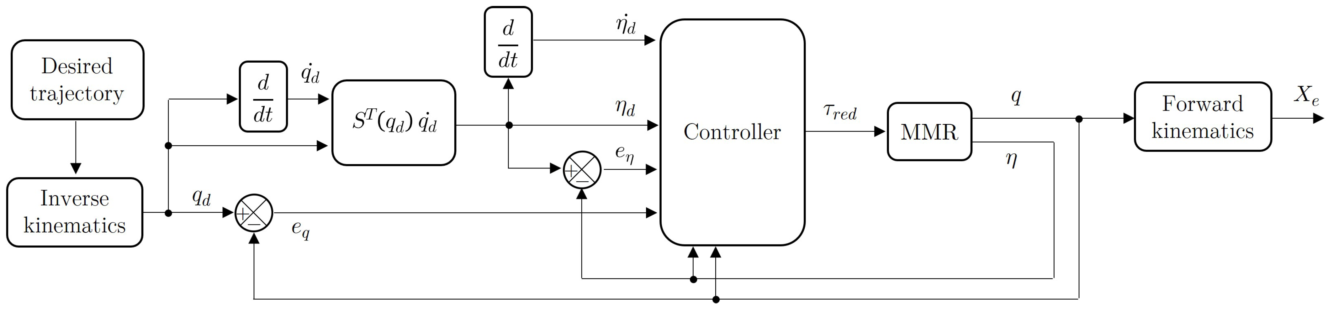
3.1. Closed-Loop Dynamics

Let
e Γ = e β e μ ,
be the complete error vector. Where the mobile platform error vector is represented by e β , and the manipulator error vector is denoted by e μ , i.e.,
e β = e r x e r y e θ e ˙ θ e v
e μ = e ϕ 1 e ˙ ϕ 1 e ϕ 2 e ˙ ϕ 2 e ϕ n m e ˙ ϕ n m .
The closed-loop dynamics are obtained by substituting (28) into the reduced model (13); for the manipulator, we obtain:
e ¨ ϕ i + k p i + 2 e ˙ ϕ i + k i + 3 e ϕ i = 0 , i = 1 , , n m ,
(32) represents a set of n m linear and decoupled systems. Considering k p i + 2 , k i + 3 > 0 , it is easy to prove asymptotic stability for states e ϕ i e ˙ ϕ i at the origin, i.e., e ϕ i e ˙ ϕ i 0 0 as t , corresponding to the manipulator angular positions and velocities. However, it is not that clear for the mobile base, whose closed-loop dynamics are represented by the set of equations:
e ˙ v + k p 1 e v + k 1 e r x = 0 e ¨ θ + k p 2 e ˙ θ + k 2 v d sin e θ e θ e r y + k 3 e θ = 0 .

3.2. Error Dynamics

Using Equations (25)–(27) and (2), it is possible to obtain:
e ˙ x = x ˙ d + e v v d cos θ d e θ e ˙ y = y ˙ d + e v v d sin θ d e θ e ˙ r x = v d cos e θ + θ ˙ d e ˙ θ e r y + e v v d e ˙ r y = e ˙ θ θ ˙ d e r x + v d sin e θ e ˙ θ = e η 2 e ˙ ϕ i = e η i + 2 , i = 1 , , n m .
The so-called error dynamics conforms the set of Equations (32)–(34).

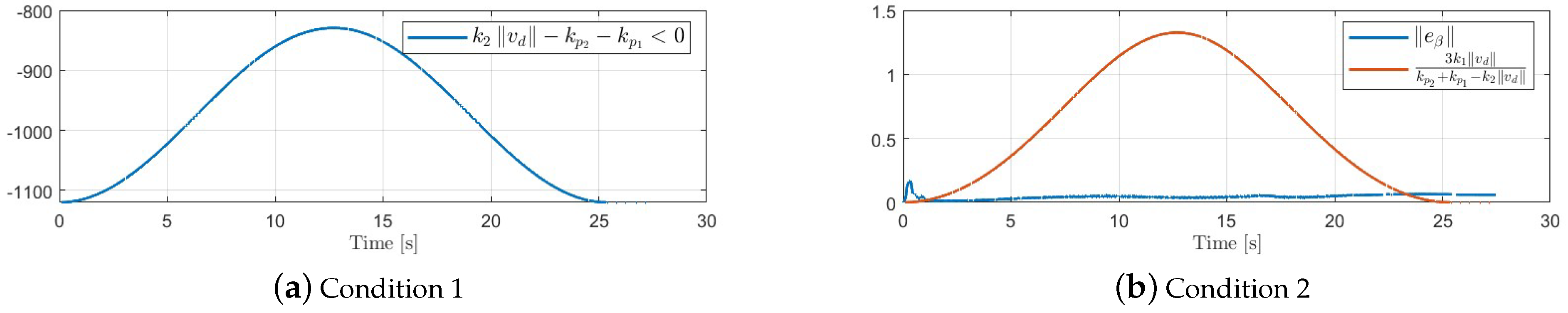
3.3. Stability Analysis

Note that there is no need to prove stability for the manipulator due to the linearization achieved in the closed-loop dynamics section, see Section 3.1 (in any case, we provide some proof of this in Appendix A). In the following, the mobile base stability is proven.
Let V e β be the proposed Lyapunov candidate function:
V e β 1 2 k 1 e r x 2 + e r y 2 + 1 2 k 3 e θ 2 + e ˙ θ 2 + e v 2 .
The time derivative of (35), considering the error dynamics, can be written as:
V ˙ e β = k 1 v d e r x cos e θ 1 + k 1 v d e r y sin e θ k 2 v d sin e θ e θ e ˙ θ e r y k p 2 e ˙ θ 2 k p 1 e v 2 .
The goal is to prove:
V ˙ e β k 1 v d e r x cos e θ 1 + k 1 v d e r y sin e θ + k 2 v d sin e θ e θ e ˙ θ e r y k p 2 e ˙ θ 2 k p 1 e v 2 0 .
Using that
e r x e β , e r y e β , e ˙ θ e β , e v e β ,
an upper bound is found for every term in (37), i.e.,
k 1 v d e r x cos e θ 1 2 k 1 v d e β k 1 v d e r y sin e θ k 1 v d e β k 2 v d sin e θ e θ e ˙ θ e r y k 2 v d e β 2 k p 2 e ˙ θ 2 k p 2 e β 2 k p 1 e v 2 k p 1 e β 2
Then, (37) is re-written as:
V ˙ e β 3 k 1 v d e β + k 2 v d k p 2 k p 1 e β 2
To assure that V ˙ e β 0 , the following conditions are established:
Condition 1. 
Gains can be chosen such that:
k 2 v d k p 2 k p 1 < 0 .
Condition 2. 
From the right hand side of (38), and considering that Condition 1 is satisfied, we have to assure that the right term is greater than the left term in magnitude; this yields an interval for the mobile base error vector norm of
e β     3 k 1 v d k p 2 + k p 1 k 2 v d .
In conclusion, we cannot guarantee asymptotic stability but rather we have an upper bound for the mobile base error norm by a positive quantity; this is termed UUB stability [20], p. 85.
Furthermore, (40) denotes a compact set, which can be made arbitrarily large by adjusting the control gains, where the system will be stable. Therefore, semiglobal stabilization is achieved [20], pp. 198–199.

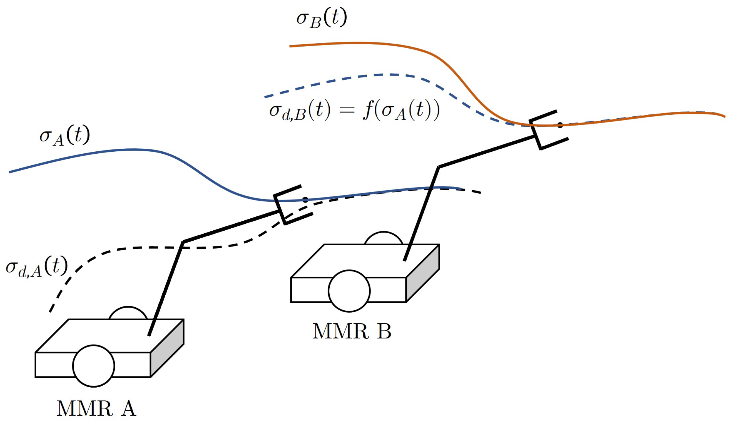
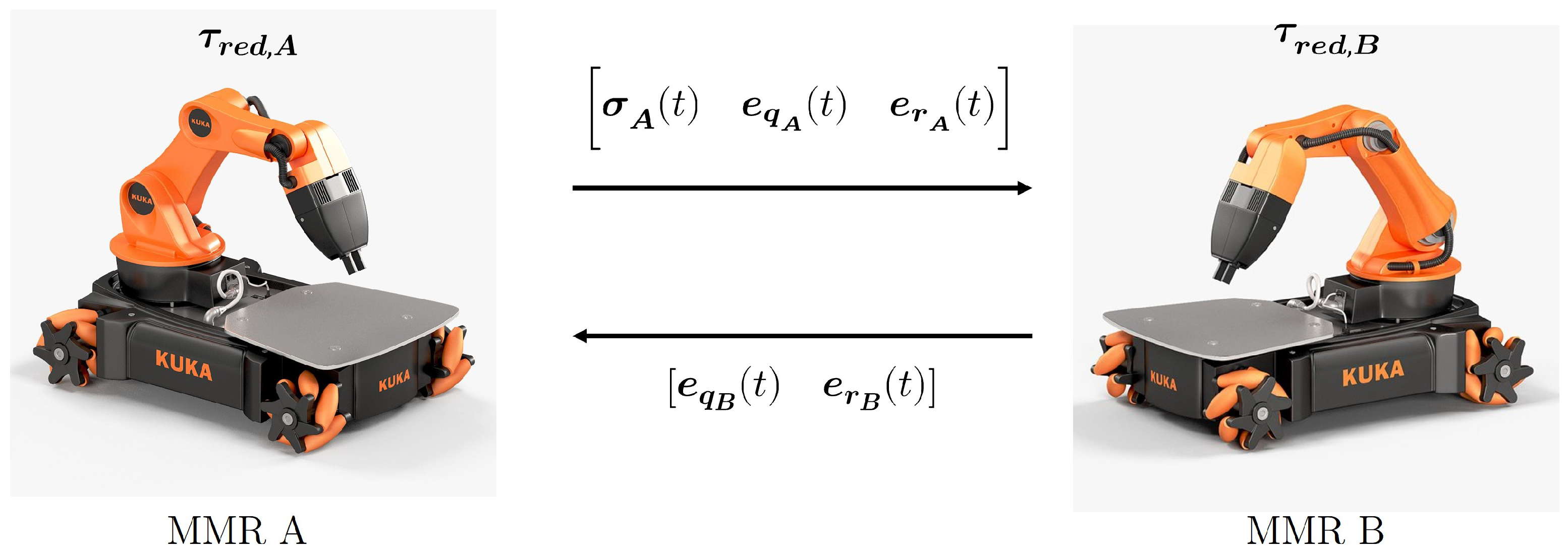
4. Synchronization Problem

Two robots A and B in a master–slave configuration, being A the “Master” and B the “Slave”, are considered, see Figure 7.
Let σ d , i ( t ) = q d , i η d , i and σ i ( t ) = q i η i be desired and actual trajectories for the i-th robot, respectively, where:
q d , i = x d , i y d , i θ d , i ϕ 1 d , i ϕ n m d , i , q i = x i y i θ i ϕ 1 , i ϕ n m , i , η d , i = v d , i θ ˙ d , i ϕ ˙ 1 d , i ϕ ˙ n m d , i , η i = v i θ ˙ i ϕ ˙ 1 , i ϕ ˙ n m , i , for i = A , B .
In this configuration, the master robot A is controlled independently of the movement of the slave robot B. For the master robot, the trajectory tracking controller posted in the previous section is used for tracking the desired trajectory σ d , A . Meanwhile, the slave reference is formed as a function of the master actual trajectories, i.e.,
σ d , B ( t ) = f σ A ( t ) ,
this constitutes a uni-directional information flow (information is passed from master to slave but not viceversa). In order to ensure feedback to the master, coupling errors for the i-th robot with respect to the j-th robot are defined:
j ϵ i R n = j e c x , i j e c y , i j e c θ , i j e c ϕ 1 , i j e c ϕ 2 , i j e c ϕ n m , i = e r x , i e r x , j e r y , i e r y , j e θ , i e θ , j e ϕ 1 , i e ϕ 1 , j e ϕ 2 , i e ϕ 2 , j e ϕ n m , i e ϕ n m , j , i j .
In a general framework, with more than two robots in the system, let us define Y as the set of robots in the whole system; Ω i Y is the subset in which the i-th robot and its neighbors with whom it shares information are found, and let N i be the number of elements in Ω i , i.e., card Ω i = N i , with card Ω i ≤ card Y . Therefore, the proposed synchronization control strategy for the i-th robot is defined as:
τ red , i = P 1 q i H q i I 1 q i , η i + η ˙ d , i + K p e η i + G * q i + F f * q i , q ˙ i + U q i , q d , i , η d , i + j Ω i N i j U s , i , i j .
where:
j U s , i R n 1 = Λ i e q i j C i j ϵ i
Λ i e q i R n 1 × n = 1 0 0 0 1 × n m 0 sin e θ , i e θ , i 1 0 1 × n m 0 n m × 1 0 n m × 1 0 n m × 1 1 n m × n m j C i R n × n = diag { j C x , i j C y , i j C θ , i j C ϕ 1 , i j C ϕ n m , i } e q i = q d , i q i e η i = η d , i η i .
j U s , i is the term that contains the static couplings for the i-th robot with respect to the j-th robot; this term is in charge to achieve synchronization. j C i is the positive definite diagonal matrix of synchronization control gains for the i-th robot; e q i and e η i are the position and velocity error vectors for the i-th robot, respectively. The remaining terms are defined in (28) with respect to the i-th robot and are similar for the j-th one.
The provided synchronization strategy allows one to design networks of robots working together in different configurations. For the sake of clarity, in this paper only the cooperative manipulation with two robots is kept; the synchronization scheme is shown in Figure 8, where e r i , i = A , B are the relative errors for the mobile base of the i-th robot, see (27). In the following, the MMR position errors are used to obtain the coupling errors, and both errors allow us to compute the control (44) for the i-th robot.
In the next section, firstly, the control performance for one MMR is experimentally tested for the trajectory tracking problem; subsequently, the master–slave scheme, using two MMRs for the synchronization problem, is simulated under the paradigm of cooperative manipulation, considering a virtual object.

5. Results

5.1. Trajectory Tracking Experimental Results

Communication with KUKA youBot is achieved using a TCP/IP protocol, through sockets. This allowed us to have active communication between a server (external computer) and a client (KUKA youBot), see Figure 9. KUKA youBot uses Ubuntu 12.04 LTS as OS, and the programming language used in the external computer was C++. The sampling time was found to be of 2.8 ms, which is small enough to consider feasible the use of the equations of the continuous system in the discrete domain.
It is actually possible to control the KUKA youBot dynamically, i.e., the robot receives torque commands from the external computer and sends information about its positions and velocities, measured on a frame established by the robot itself, that we denoted as frame {m}, as feedback. To obtain the states needed for computing the control τ red , a coordinate transformation was made.
Considering Figure 10, we defined ( x i , y i , ϑ i ) as the initial pose for the KUKA youBot mobile base on the inertial frame {0}. The initial pose for the KUKA youBot mobile base is constant (i.e., ( x i , y i , ϑ i ) are not time-varying), where the robot defines its own inertial frame named {m}.
The robot sends the states ( x m , y m , θ m ) to the computer, which correspond to the position and orientation for the mobile base on the horizontal plane measured with respect to {m}, and to longitudinal and angular velocity ( v , θ ˙ m ) and ( ϕ i , ϕ ˙ i ) , respectively, with i = 1 , , 5 for the manipulator angular positions and velocities.
To obtain the states measured on inertial frame {0}, the next transformation was considered:
x = x i + x m cos ϑ i y m sin ϑ i y = y i + y m cos ϑ i + x m sin ϑ i x ˙ = x ˙ m cos ϑ i y ˙ m sin ϑ i y ˙ = y ˙ m cos ϑ i + x ˙ m sin ϑ i θ = ϑ i + θ m θ ˙ = θ ˙ m .
where:
x ˙ m = v cos ( θ m ) , y ˙ m = v sin ( θ m ) .
According with the first assumption made on Section 2.3 for the mobile base, namely, the two wheels of each side rotate at the same speed; the next torques relation is considered, see Figure 11:
τ r 0 = τ r 2 = τ i 2 , τ r 1 = τ r 3 = τ d 2 .
Control actions were bounded (in code) as follows:
10 N · m τ d , τ i , τ 5 10 N · m 15 N · m τ 1 , τ 2 , τ 3 , τ 4 15 N · m .
The desired trajectory is defined as a circle with center at ( x c , y c ) = ( 1 , 0 ) , radius r d = 1 for the mobile base, and radius r e f = 1.3 for the end-effector, i.e.,
δ t = 2 π t f t sin 2 π t f t x d t = x c + r d cos δ t y d t = y c + r d sin δ t , δ e f t = δ t + sin 1 L x r e f x e f d t = x c + r e f cos δ e f t y e f d t = y c + r e f sin δ e f t z e f d t = 0.46 .
This planning was thought for a time t f = 24 s.
θ d is computed as follows:
θ d t = π / 2 + 2 π n c , if x ˙ d , y ˙ d = 0 atan 2 y ˙ d , x ˙ d + 2 π n c , if y ˙ d > 0 and x ˙ d < 0 atan 2 y ˙ d , x ˙ d + 2 π + 2 π n c , if y ˙ d < 0 or x ˙ d , y ˙ d > 0 .
where n c is the number of cycles given by the mobile base. For this experiment, just one cycle is considered, and this counter takes the value of n c = 1 at the end of the trajectory, i.e., at t = t f .
Notice that the proposed trajectory starts and finishes with v d = 0 . To avoid singularities for θ ˙ d ( t ) in (24), it is possible to set θ ˙ d ( t ) = 0 when v d ( t ) = 0 artificially, in code; however, we cannot expect the stability condition (40) to be satisfied when this happens, see Figure 12.
The end-effector desired orientations are defined as:
ψ e f d t = π 2 , ζ e f d t = θ d π 2 .
All the initial conditions were set to 0, except for θ ( 0 ) = π / 2 .
Finally, with the parameters shown in Table A1 (these parameters are not exactly known; uncertainties exist, and some of them where calculated or supposed), and control gains are shown in Table 1; performance charts were obtained, see Figure 13.
The video of the experiment is shown in the following link: https://drive.google.com/file/d/1We9XsklA2-GLTUxg973DUmGcWTJm1zAz/view, accessed on 7 September 2023.

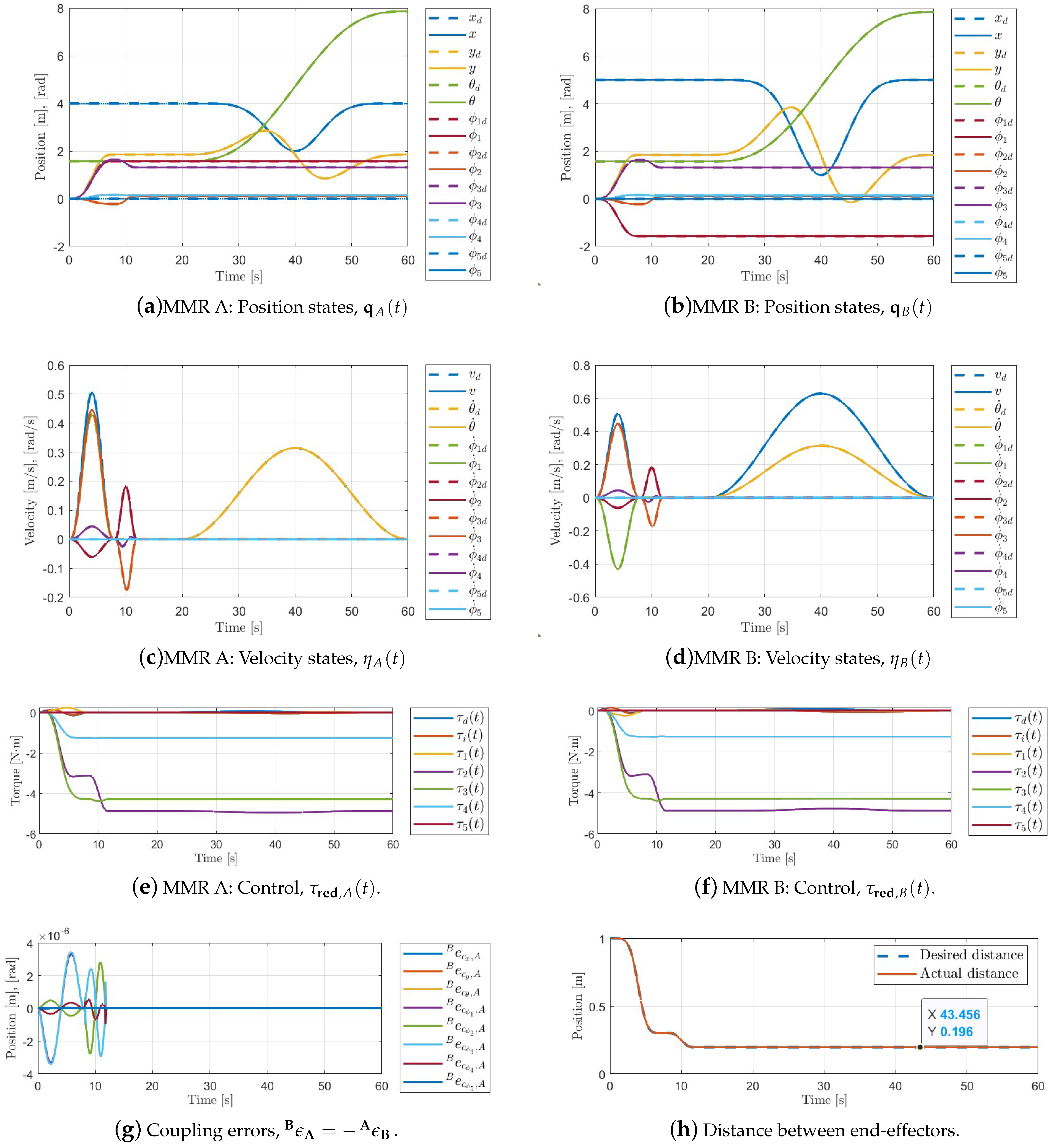
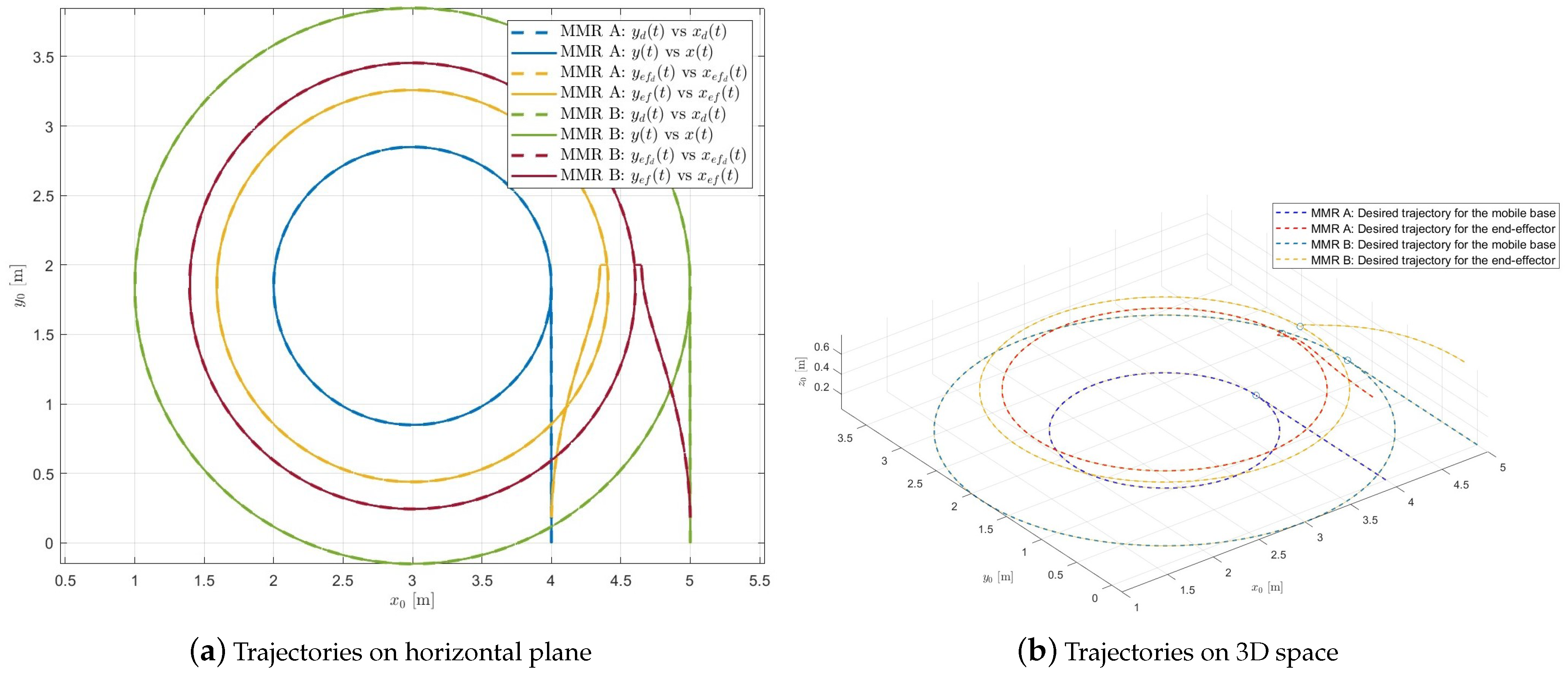
5.2. Synchronization: Numerical Simulations

In this simulation, two KUKA youBot robots (A and B) with n = 8 DoF, being A the master and B the slave, are considered. Coupling errors shown in (43) and control (44) with i , j = A , B were used.
The task is about manipulating a 20 cm side length virtual box along a circular trajectory, i.e., robots have to guarantee the grip of an object maintaining the distance among the end-effectors while the trajectory is executed. Emphasizing on the word virtual, in this work, the interaction with the environment is neglected, and the term J e ( q ) h r , in models (6) and (13), is considered zero.
The trajectory planning is defined by four stages:
  • The first stage: The robot mobile base describes a straight line until the box position is reached, and the manipulator is positioned in front of the object.
  • The second stage: In this stage, the end-effector makes contact with the object in a smooth manner. It is considered a punctual grip (without friction); thus, a perpendicular grip with the object is required.
  • The third stage: This stage is about maintaining the position for a few seconds in order to wait for the effects of tapping that may exist between the object and the end-effector to pass, and for the grip to reach a point of stability.
  • The fourth stage: The robots generate the desired circle.
The object position is considered at ( 4.5 , 2 , 0.46 ) on frame {0}, and the initial position of the mobile base is at ( 4.5 , 0 ) . The trajectory planning is defined as follows:
The first stage, 0 t 8 s:
For robot A, the desired trajectories are defined as:
p 1 t = 5 t 7 524288 + 35 t 6 131072 21 t 5 8192 + 35 t 4 4096 x d , A t = 4 y d , A t = 2 L x p 1 t , x e f d , A t = 8 = 4.35 y e f d , A t = 8 = y d , A t = 8 + L x z e f d , A t = 8 = 0.46 ψ e f d , A t = 8 = π 2 ζ e f d , A t = 8 = 0 .
To obtain reasonable control actions in the manipulator, the function p 1 ( t ) is used to interpolate the trajectory from the initial point to the last, softly, for every link, i.e.,
ϕ 1 d , A t = π 2 p 1 t ϕ 2 d , A t = 0.222635 p 1 t ϕ 3 d , A t = 1.63105 p 1 t ϕ 4 d , A t = 0.162383 p 1 t .
For robot B, the desired trajectories are defined as:
q d , B = W q s 1 , 2 , 3 q A + Q q s 1 , 2 , 3 , η d , B = W η s 1 , 2 , 3 η A .
where:
W q s 1 , 2 , 3 = diag { 1 1 1 1 1 1 1 1 } , W η s 1 , 2 , 3 = diag { 1 1 1 1 1 1 1 } , Q q s 1 , 2 , 3 = 1 0 1 × 7 .
The second stage, 8 < t 12 s:
For robot A, the desired trajectories are defined as follows:
x d , A t = 4 y d , A t = 2 L x , p 2 t = 35 t 4 2 4 84 t 4 2 5 + 70 t 4 2 6 20 t 4 2 7 x e f d , A t = 4.4 + ρ d 4.35 p 2 t + 4.35 y e f d , A t = 2 z e f d , A t = 0.46 ψ e f d , A t = π 2 ζ e f d , A t = 0 .
where ρ d is a desired penetration on the virtual object to guarantee the grip.
For robot B, the desired trajectories are defined as in Equation (52).
The third stage, 12 < t 20 s:
For robot A, the desired trajectories are defined as follows:
x d , A t = 4 y d , A t = 2 L x , x e f d , A t = 4.4 + ρ d y e f d , A t = 2 z e f d , A t = 0.46 ψ e f d , A t = π 2 ζ e f d , A t = 0 .
For robot B, the desired trajectories are defined as in Equation (52).
The fourth stage, 20 < t t f = 60 s:
For this stage, a circle with center at ( x c , y c ) = ( 3 , 2 L x ) and radius r d , A = 1 m on the horizontal plane for the robot A mobile base is considered, and the end-effector has a radius r e f , A = L x 2 + r d , A + 0.4 + ρ d 2 . Therefore, the desired trajectories for robot A are defined as:
δ A t = 2 π t f 20 t 20 sin 2 π t f 20 t 20 x d , A t = x c + r d , A cos δ A t y d , A t = y c + r d , A sin δ A t , δ e f , A t = δ A t + sin 1 L x r e f , A x e f d , A t = x c + r e f , A cos δ e f , A t y e f d , A t = y c + r e f , A sin δ e f , A t z e f d , A t = 0.46 ψ e f d , A t = π 2 ζ e f d , A t = θ d , A t π 2 .
For the robot B mobile base, a circle with the same center ( x c , y c ) = ( 3 , 2 L x ) but with radius r d , B = r d , A + 1 is considered. The desired trajectories are defined as:
q d , B = Q q s 4 + W q s 4 ( q A Q q s 4 ) , η d , B = W η s 4 η A .
where:
W q s 4 = diag { r d , B r d , A r d , B r d , A 1 1 1 1 1 1 } , W η s 4 = diag { r d , B r d , A 1 1 1 1 1 1 } , Q q s 4 = x c y c 0 1 × 6
In general, ϕ 5 d , A ( t ) = 0 for all t and θ d , A ( t ) is computed using (49). The functions p 1 ( t ) and p 2 ( t ) are soft polynomials, generated with the method based on Bezier curves presented in [21], such that their first time-derivative at the beggining and at the end of the trajectory is zero.
Initial conditions are considered as 0 for positions ( q i ( 0 ) ) and velocities ( η i ( 0 ) ) for both robots, i = A , B , except for the mobile base position: for robot A, ( x A ( 0 ) , y A ( 0 ) , θ A ( 0 ) ) = ( 4 , 0 , π / 2 ) is considered; and for robot B, ( x B ( 0 ) , y B ( 0 ) , θ B ( 0 ) ) = ( 5 , 0 , π / 2 ) .
The control gains for both robots A and B are shown in Table 2, and the coupling gains are shown in Table 3. A desired penetration of ρ d = 0.002 m on the object is considered.
Performance charts are shown in Figure 14, and trajectories are presented in Figure 15.
The simulation was animated on CoppeliaSim, and the video is shown in the next link: https://drive.google.com/file/d/1Z4RWykuw5bglV7KKbzTZKf0beEjUXghi/view?usp=sharing, accessed on 7 September 2023.

6. Discussion

A non-linear control law for a n DoF MMR with semiglobal and UUB stability properties for solving the trajectory tracking problem, considering movement (kinematic) constraints, was designed and tested on the experimental platform KUKA youBot. Reasonable control actions, the acomplishment of the non-holonomic constraint, and small position and velocity errors were achieved with a maximum position error of 6 cm, see Figure 13, even in the presence of parametric uncertainties and unmodeled dynamics. The stability conditions were validated when v d 0 , see Figure 12; notice that condition 2 is violated when v d = 0 , as expected.
The trajectory tracking control designed was extended to the synchronization notion, which is valid for both uni-directional or bi-directional information flow between robots, and for any number of robots in a given network through static couplings considering a master–slave configuration. Numerical simulation considering 2 KUKA youBot models and a manipulation task using a 20 cm virtual box was developed in the CoppeliaSim environment. From Figure 14, reasonable control actions and really small errors for both robots can be observed. The grip of the box is guaranteed maintaining a distance between the end-effectors of 19.6 cm, as expected, since the desired penetration ( ρ d ) on the object of 2mm was considered of for each robot.
The generalized MMR model has been formulated considering the simplest friction model viscous, i.e., f f i = b q i q ˙ i is the i-th element of F f ( q , q ˙ ) with b q i viscous friction coefficients. Friction forces could be up to the 25% of the torque required to move a manipulator [22], as future work is considered to use a more fit friction model as the LuGre model.
Regarding the synchronization approach, experimental validation is expected for future works. Moreover, adding velocity-level coupling terms and changing to dynamical couplings instead of static couplings is also envisioned. In this work, we have supposed a virtual box as a manipulated object to validate the synchronization control on simulation. In the manipulation sense, when robots are interacting with their environment, the term J e ( q ) h r in (6) and (13) becomes relevant for the dynamics of the system; to this end, adding a force controller in the MMR’s end-effector print on the object for manipulation purposes will be also desirable, leading to the design of a hybrid position/force controller.
Finally, given the parametric uncertainties and non-modeled dynamics on the system, adding an adaptation law or use a parameter estimator would address the robustness of the controller.

Author Contributions

Conceptualization, J.G.P.-F., A.B.M.-D. and A.R.-Á.; methodology, J.G.P.-F., A.B.M.-D. and A.R.-Á.; software, J.G.P.-F.; validation, J.G.P.-F.; formal analysis, J.G.P.-F., A.B.M.-D. and A.R.-Á.; investigation, J.G.P.-F., A.B.M.-D. and A.R.-Á.; writing—original draft preparation, J.G.P.-F.; writing—review and editing, J.G.P.-F., A.B.M.-D. and A.R.-Á.; and supervision, A.B.M.-D. and A.R.-Á. All authors have read and agreed to the published version of the manuscript.

Funding

This research was funded by Consejo Nacional de Ciencia y Tecnología, grant number 1079389; and Centro de Investigación y de Estudios Avanzados del Instituto Politécnico Nacional, grant number IE-ES-2022-123. The authors are also grateful for the support through the project SEP CONACYT CB2017-2018-A1-S-26123: “Análisis, control y sincronización de sistemas complejos con interconexiones dinámicas y acoplamientos flexibles”.

Institutional Review Board Statement

Not applicable.

Informed Consent Statement

Not applicable.

Data Availability Statement

Not applicable.

Acknowledgments

The authors are grateful for the support through the project SEP CONACYT CB2017-2018-A1-S-26123.

Conflicts of Interest

The authors declare no conflict of interest.

Abbreviations

The following abbreviations are used in this manuscript:
MDPIMultidisciplinary Digital Publishing Institute
MMRMobile manipulator robot
UUBUniformly and ultimately boundedness
DoFDegrees of freedom
CoMCenter of mass
OSOperating system

Appendix A. Manipulator Stability

Let us re-write the set of Equations (32) for a n m DoF manipulator as follows:
e ¨ ϕ i = k p i + 2 e ˙ ϕ i k i + 3 e ϕ i , i = 1 , 2 , , n m .
With k p i + 2 , k i + 3 > 0 and e ϕ i e ˙ ϕ i T constituting the state-vector, where e ϕ i is the angular position error for the i-th link and e ˙ ϕ i the angular velocity error.
Then, let
V e μ 1 2 e ˙ ϕ i 2 + 1 2 k i + 3 e ϕ i 2 ,
the proposed Lyapunov candidate function. Taking the time-derivative of Equation (A2) along the trajectories of the system (A1), we obtain:
V ˙ e μ = k p i + 2 e ˙ ϕ i 2 0 .
Since k p i + 2 > 0 , notice that V ˙ e μ = 0 only when e ˙ ϕ i = 0 , but the position error vector e ϕ i could “get stuck” in any other value. In order to analyze this situation, consider the system (A1) when e ˙ ϕ i = 0 —this implies having e ¨ ϕ i = 0 ; then, we obtain:
k i + 3 e ϕ i = 0 , i = 1 , 2 , , n m .
Since k i + 3 > 0 , the only solution is e ϕ i = 0 . Thus, the only invariant set that satisfies V ˙ = 0 is the origin e ϕ i e ˙ ϕ i = 0 0 . Therefore, according to LaSalle, it can be concluded that the system is globally asymptotically stable.

Appendix B. Technical Data for KUKA youBot

Some technical data and parameters for KUKA youBot can be found at [23]; in this paper, limitations on the arm angular positions and velocities have been considered, especially the limitation on the mobile base longitudinal velocity, v 0.8 m/s, which was fundamental for the trajectory planning.
The parameters that were used for experimental validation are shown in Table A1:
Table A1. KUKA youBot physical parameters.
ParameterValueParameterValueParameterValue
m m [kg]19.803 L c b [m]0.036 I 2 z z [kg · m 2 ]0.0031631
m b [kg]0.961 L c 1 [m]0.058 I 3 x x [kg · m 2 ]0.00041967
m 1 [kg]1.390 L c 2 [m]0.11397 I 3 y y [kg · m 2 ]0.00172767
m 2 [kg]1.318 L c 3 [m]0.104 I 3 z z [kg · m 2 ]0.0018468
m 3 [kg]0.821 L c 4 [m]0.053 I 4 x x [kg · m 2 ]0.0006610
m 4 [kg]0.769 L c 5 [m]0.016 I 4 y y [kg · m 2 ]0.0006764
m 5 [kg]0.906 r b [m]0.033 I 4 z z [kg · m 2 ]0.0010573
h b [m]0.030 r c [m]0.0255 I 5 x x [kg · m 2 ]0.0005563
h c [m]0.110 L x [m]0.151 I 5 y y [kg · m 2 ]0.0003926
R [m]0.050 I m x x [kg · m 2 ]0.2657 I 5 z z [kg · m 2 ]0.0002756
p x [m]0 I m y y [kg · m 2 ]0.5875 b x [N s/m]0.8
p y [m]0 I m z z [kg · m 2 ]0.5875 b y [N s/m]0.8
p z [m]-0.001 I b x x [kg · m 2 ]0.00041515 b θ [N s/m]0.7
L [m]0.150 I b y y [kg · m 2 ]0.003553778 b ϕ 1 [N s/m]0.5
L b [m]0.072 I b z z [kg · m 2 ]0.00041515 b ϕ 2 [N s/m]0.5
L 1 [m]0.075 I 1 x x [kg · m 2 ]0.0058821 b ϕ 3 [N s/m]0.5
L 2 [m]0.155 I 1 y y [kg · m 2 ]0.0029525 b ϕ 4 [N s/m]0.5
L 3 [m]0.135 I 1 z z [kg · m 2 ]0.0060091 b ϕ 5 [N s/m]0.5
L 4 [m]0.081 I 2 x x [kg · m 2 ]0.0005843
L 5 [m]0.137 I 2 y y [kg · m 2 ]0.0031145

References

  1. Wang, C.; Sun, D. A synchronization control strategy for multiple robot systems using shape regulation technology. In Proceedings of the 2008 7th World Congress on Intelligent Control and Automation, Chongqing, China, 25–27 June 2008; pp. 467–472. [Google Scholar] [CrossRef]
  2. Markus, E.D. Differential Flatness Based Synchronization Control of Multiple Heterogeneous Robots. In Proceedings of the IECON 2018-44th Annual Conference of the IEEE Industrial Electronics Society, Washington, DC, USA, 21–23 October 2018; pp. 3659–3664. [Google Scholar] [CrossRef]
  3. Fathallah, M.; Abdelhedi, F.; Derbel, N. Synchronization of multi-robot manipulators based on high order sliding mode control. In Proceedings of the 2017 International Conference on Smart, Monitored and Controlled Cities (SM2C), Sfax, Tunisia, 17–19 February 2017; pp. 138–142. [Google Scholar] [CrossRef]
  4. Cicek, E.; Dasdemir, J. Output feedback synchronization of multiple robot systems under parametric uncertainties. Trans. Inst. Meas. Control 2017, 39, 277–287. [Google Scholar] [CrossRef]
  5. Cicek, E.; Dasdemir, J.; Zergeroglu, E. Coordinated synchronization of multiple robot manipulators with dynamical uncertainty. Trans. Inst. Meas. Control 2015, 37, 672–683. [Google Scholar] [CrossRef]
  6. Portillo-Vélez, R.d.J.; Cruz-Villar, C.A.; Rodríguez-Ángeles, A. On-line master/slave robot system synchronization with obstacle avoidance. Stud. Inform. Control 2012, 21, 17–26. [Google Scholar] [CrossRef]
  7. Zhao, X.; Zhang, Y.; Ding, W.; Tao, B.; Ding, H. A Dual-Arm Robot Cooperation Framework Based on a Nonlinear Model Predictive Cooperative Control. IEEE/ASME Trans. Mechatron. 2023, 1–13. [Google Scholar] [CrossRef]
  8. Rosales-Hernández, F.; Velasco-Villa, M.; Castro-Linares, R.; del Muro-Cuéllar, B.; Hernández-Pérez, M.Á. Synchronization strategy for differentially driven mobile robots: Discrete-time approach. Int. J. Robot. Autom. 2015, 30, 50–59. [Google Scholar] [CrossRef]
  9. Sun, D.; Wang, C.; Shang, W.; Feng, G. A Synchronization Approach to Trajectory Tracking of Multiple Mobile Robots While Maintaining Time-Varying Formations. IEEE Trans. Robot. 2009, 25, 1074–1086. [Google Scholar] [CrossRef]
  10. Li, H.; Jiang, W.; Zou, D.; Yan, Y.; Zhang, A.; Chen, W. Robust motion control for multi-split transmission line four-wheel driven mobile operation robot in extreme power environment. Ind. Robot. Int. J. Robot. Res. Appl. 2020. ahead-of-print. [Google Scholar] [CrossRef]
  11. Algrnaodi, M.; Saad, M.; Saad, M.; Fareh, R.; Kali, Y. Extended state observer–based improved non-singular fast terminal sliding mode for mobile manipulators. Trans. Inst. Meas. Control 2023. ahead-of-print. [Google Scholar] [CrossRef]
  12. Shafei, A.M.; Mirzaeinejad, H. A novel recursive formulation for dynamic modeling and trajectory tracking control of multi-rigid-link robotic manipulators mounted on a mobile platform. Proc. Inst. Mech. Eng. Part I J. Syst. Control Eng. 2020, 235, 1204–1217. [Google Scholar] [CrossRef]
  13. Portillo Vélez, R.d.J. Control Multilateral de Agarre para Robots Cooperativos Maestro/Multi-Esclavo. Ph.D. Thesis, CINVESTAV, Zacatenco, Mexico, 2013. [Google Scholar]
  14. Fierro, R.; Lewis, F. Control of a nonholonomic mobile robot: Backstepping kinematics into dynamics. In Proceedings of the 1995 34th IEEE Conference on Decision and Control, New Orleans, LA, USA, 13–15 December 1995; Volume 4, pp. 3805–3810. [Google Scholar] [CrossRef]
  15. Bischoff, R.; Huggenberger, U.; Prassler, E. KUKA youBot—A mobile manipulator for research and education. In Proceedings of the 2011 IEEE International Conference on Robotics and Automation, Shanghai, China, 9–13 May 2011; pp. 1–4. [Google Scholar] [CrossRef]
  16. Galati, R.; Mantriota, G. Path Following for an Omnidirectional Robot Using a Non-Linear Model Predictive Controller for Intelligent Warehouses. Robotics 2023, 12, 78. [Google Scholar] [CrossRef]
  17. Wang, T.; Wu, Y.; Liang, J.; Han, C.; Chen, J.; Zhao, Q. Analysis and Experimental Kinematics of a Skid-Steering Wheeled Robot Based on a Laser Scanner Sensor. Sensors 2015, 15, 9681–9702. [Google Scholar] [CrossRef] [PubMed]
  18. Fuentevilla, G. Definiciones del Modelo KUKA youBot. 2022. Available online: https://drive.google.com/file/d/1O_iH2lNSz0y-z2rv-nDqPhUTe0-oBxVb/view?usp=sharing (accessed on 7 September 2023).
  19. Gutiérrez, H.; Morales, A.; Nijmeijer, H. Synchronization Control for a Swarm of Unicycle Robots: Analysis of Different Controller Topologies. Asian J. Control 2017, 19, 1822–1833. [Google Scholar] [CrossRef]
  20. Khalil, H.K. Nonlinear Control; Pearson Education: Upper Saddle River, NJ, USA, 2015. [Google Scholar]
  21. Gómez León, B.C. Control de Manipulador Móvil Subactuado, Provisto de Unión Flexible. Master’s Thesis, CINVESTAV, Zacatenco, Mexico, 2021. [Google Scholar]
  22. Craig, J.J. Introduction to Robotics: Mechanics and Control; Pearson Education: Upper Saddle River, NJ, USA, 2005. [Google Scholar]
  23. MediaWiki. Main Page-youBot Wiki. 2015. Available online: http://www.youbot-store.com/wiki/index.php/Main_Page (accessed on 7 September 2023).
Figure 1. n DoF MMR configuration.
Machines 11 00962 g001
Figure 2. Forces and torques description on the mobile platform.
Machines 11 00962 g002
Figure 3. KUKA youBot.
Machines 11 00962 g003
Figure 4. KUKA youBot configuration.
Machines 11 00962 g004
Figure 5. Relative errors on differential robot local frame in a leader-follower scheme.
Machines 11 00962 g005
Figure 6. Proposed control block diagram for MMR.
Machines 11 00962 g006
Figure 7. Master–slave scheme.
Machines 11 00962 g007
Figure 8. Bi-directional flow information between two KUKA youBot robots.
Machines 11 00962 g008
Figure 9. Communication with KUKA youBot.
Machines 11 00962 g009
Figure 10. Inertial frames and coordinates relationship.
Machines 11 00962 g010
Figure 11. Torque positive directions on robot wheels.
Machines 11 00962 g011
Figure 12. Stability conditions: numerical verification.
Machines 11 00962 g012
Figure 13. KUKA youBot performance.
Machines 11 00962 g013
Figure 14. KUKA youBot synchronization performance.
Machines 11 00962 g014
Figure 15. KUKA youBot trajectories.
Machines 11 00962 g015
Table 1. Trajectory tracking control gains.
k 1 k 2 k 3 k 4 k 5 k 6 k 7 k 8 k p 1 k p 2 k p 3 k p 4 k p 5 k p 6 k p 7
7005553001000100020002500100400720350350350350350
Table 2. Control gains for robots A and B.
k 1 k 2 k 3 k 4 k 5 k 6 k 7 k 8 k p 1 k p 2 k p 3 k p 4 k p 5 k p 6 k p 7
505020040040040040040050505050505050
Table 3. Coupling gains for robots A and B.
C x , A C y , A C θ , A C ϕ 1 , A C ϕ 2 , A C ϕ 3 , A C ϕ 4 , A C ϕ 5 , A C x , B C y , B C θ , B C ϕ 1 , B C ϕ 2 , B C ϕ 3 , B C ϕ 4 , B C ϕ 5 , B
200200200200200200200200800800800800800800800800
Disclaimer/Publisher’s Note: The statements, opinions and data contained in all publications are solely those of the individual author(s) and contributor(s) and not of MDPI and/or the editor(s). MDPI and/or the editor(s) disclaim responsibility for any injury to people or property resulting from any ideas, methods, instructions or products referred to in the content.

