1. Introduction
Continuum robots have become a topic of recent research, mainly owing to their ability to mimic the movement of certain animals such as snakes [
1], elephants (trunks) [
2] and octopuses (tentacles) [
3]. These robots are made up of flexible materials possessing good ability of bending and dexterity to maneuver in congested environments through shape morphing [
4]. Specific applications include medical surgery [
5], nuclear reactor maintenance [
6], disaster relief [
7] and other industrial uses [
8].
Continuum robots are often kinematically redundant and highly nonlinear, rendering their kinematic analysis more complex than their rigid-link counterparts. Unlike the rigid robots where the pose of any point in the robot workspace can be fully defined by link lengths and joint angles, the kinematics of continuum robots remains challenging to solve due to the under-determined nature of the underlying problem.
Substantial research has been carried out in the past. Jones and Walker [
9,
10] developed a modified homogenous transformation matrix in terms of Denavit–Hartenberg (D-H) parameters to analyze the kinematics of the continuum robot. Simaan et al. [
11] proposed a differential method to divide the continuum robot into several small units and then computed the position of the end-effector by using an integration method. Godage et al. [
12] presented a new three-dimensional kinematic model for multisection continuum arms using a shape-function-based approach and incorporating geometrically constrained structures [
13]. Another interesting approach was presented in [
14], where the authors used torus segments to represent the sections of a continuum robot called a bionic handling assistant (BHA) manipulator. Escande et al. [
15] put forward a forward kinematics model for the compact bionic handling assistant (CBHA) based on the constant curvature assumption. The above-mentioned methods share a common problem in that the inverse kinematics cannot be directly derived from the forward kinematics. Usually, numerical methods such as Least Squares [
16] and Newton–Raphson methods [
17] are adopted, but they are computationally intensive and not applicable for real-time applications. Because of this reason, qualitative methods have also been explored. Giorelli et al. [
18] modeled the inverse kinematics (IK) of a flexible manipulator using feed-forward Neural Networks (NN). Rolf and Steil [
19] introduced a goal babbling approach to solve the IK of the bionic handling assistant robot. Melingui et al. [
20] used the NN through a distal supervised learning scheme to solve the IK of the CBHA robot. Although the accuracy has been improved, these methods are still time-consuming and computationally expensive.
In conclusion, using the existing methods to solve the kinematics of the continuum robot mainly has the following problems: it is impossible or difficult to find the inverse kinematic solution, the calculation is large and the accuracy of the results is low. For these reasons, we are exploring a simple approach to solving the inverse kinematics for real-time applications.
The rest of this paper is arranged as follows.
Section 2 describes the forward kinematics based on the long beam theory. In
Section 3, the DOFs are analyzed to determine the number of parameters to be controlled. In
Section 4, a simplified model is proposed to solve the inverse kinematics of a flexible parallel robot based on the experimental studies. At last, a number of case studies are supplied to show the effectiveness of the method.
3. Mobility Analysis of the Continuum Robot
For the purpose of understanding the problem at hand, a mobility analysis may be necessary in order to determine the number of parameters involved in the inverse kinematics. This analysis is conducted based on a pseudo-rigid-body model that is usually feasible when the end of a flexible beam is of interest. Previous studies have validated the pseudo-rigid-body models, such as 1R [
22,
23,
24], 2R [
25], 3R [
26] and PR [
27].
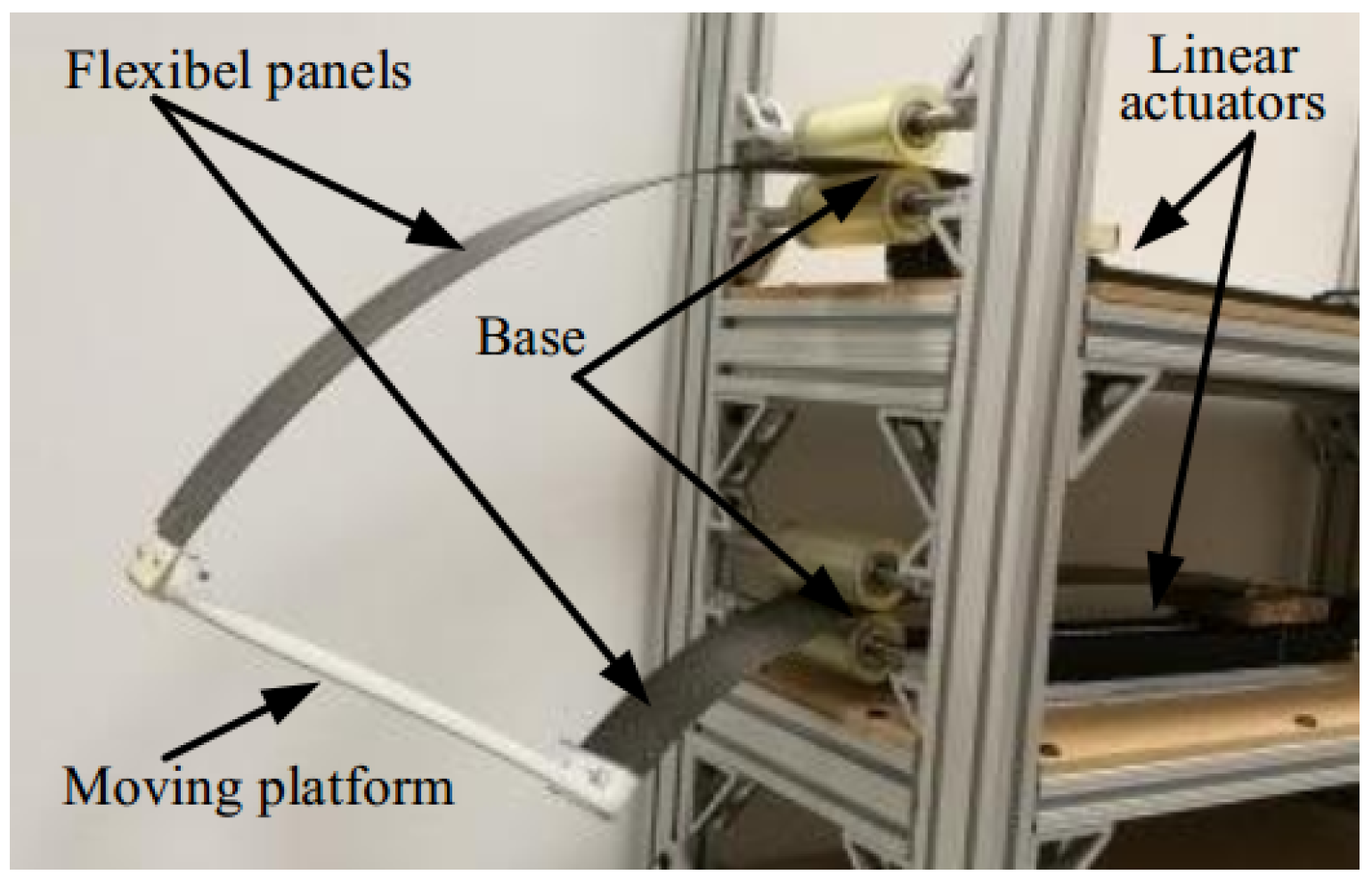
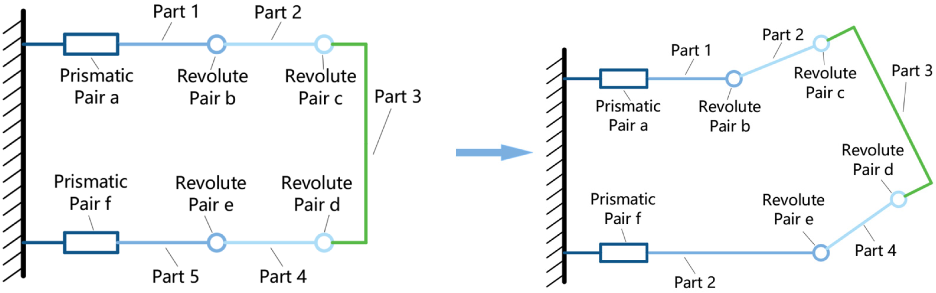
By using a 2R pseudo-rigid-body model, a sliding flexible panel can be simplified as a PRR link, with the P joint for sliding, the first R joint for bending deflection (vertical) and the second R joint for bending curvature. As shown in
Figure 3, the flexible panel mechanism is modeled by five rigid parts (part 1 to part 5), two planar prismatic pairs (pair a and pair f) and four revolute pairs (pair b to pair e). Among them, pair a and pair f represent the sliding motion of the upper and lower panels driven by their respective linear actuators. Correspondingly, pair b to pair e represent the bending deflections of the two panels and their bending curvatures. With this model, the DOFs of our robot can be calculated as
where
is the degrees of freedom (DOFs) of this mechanism,
is the number of links, i.e.,
, and
represents the number of low pair joints, i.e.,
Therefore, the DOFs of this mechanism are
. Thus, if three parameters, i.e., the position and orientation of the continuum mechanism
X,
Z and
β, are fully defined, the mechanism can be well controlled. In other words, though there are only two actuators for three pose parameters, which is traditionally considered as under-actuation, the flexibility of the panels adds additional degrees of freedom that are used for full pose control of the robot, a very interesting finding that sets a base for our work on the inverse kinematics.
4. A Quasi-Rigid Model for Inverse Kinematics
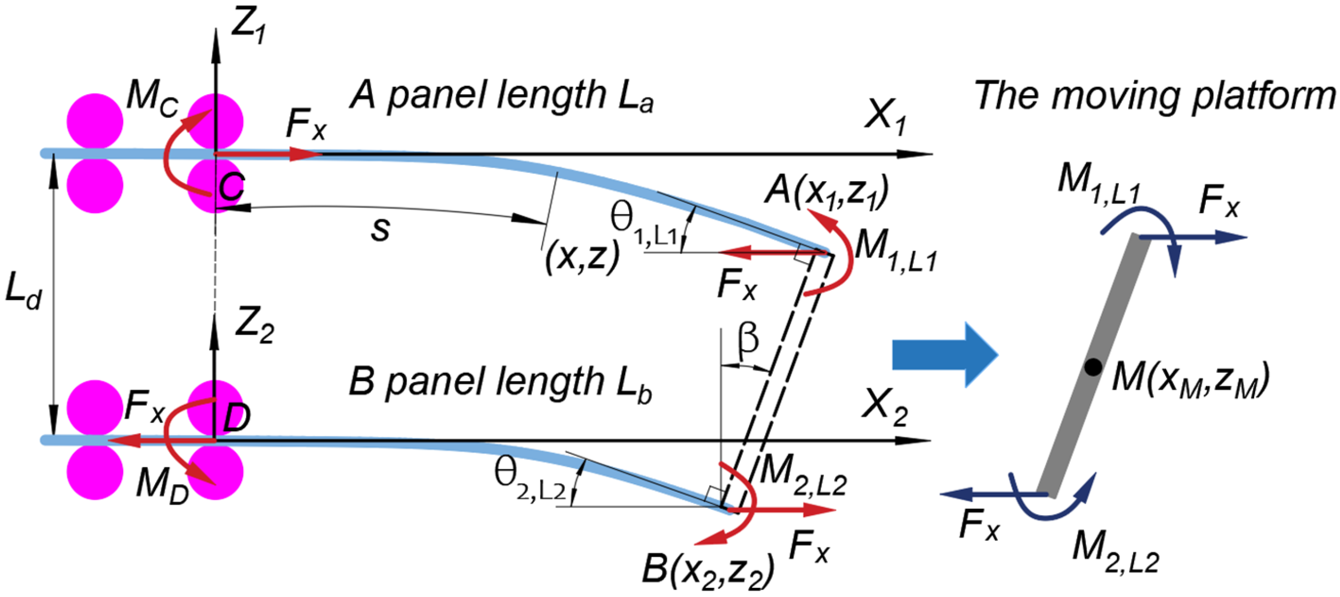
Knowing that our continuum robot can realize full pose control, we propose a quasi-rigid model for solving its inverse kinematics for real-time applications. To achieve this goal, first we conducted a series of experiments by inputting the panel lengths and then measuring the end positions of the two panels by an optical coordinated machine measurement (CMM) device from Northern Digital Polaris Vicra. As shown in
Figure 4a, by using the two end points A
and B
, we can calculate the middle point of the moving platform and its orientation as defined before as
,
and tip angle
in Equations (9) and (10).
Table 1 records the experimental data in terms of panel lengths
La and
Lb. In the experiment, both panels start from 150 mm and end at 400 mm. In total, there are five series with an increment of 50 mm for
Lb, and within each series
La changes in an increment of 50 mm. For series 1,
Lb is at the initial position of 150 mm and
Lb changes from 200 mm to 400 mm in an increment of 50 mm. For series 2,
Lb advances to 200 mm and
La changes from 250 mm to 400 mm in an increment of 50 mm. Note that this robot is symmetric along the horizontal axis;
La does not have to start from the initial position at 150 mm, as this case is already covered by series 1. For series 3, 4 and 5,
Lb advances to 250 mm, 300 mm and 350 mm, respectively, while
La starts after the respective
Lb values for the same reason. As a result, both panels are taken into consideration.
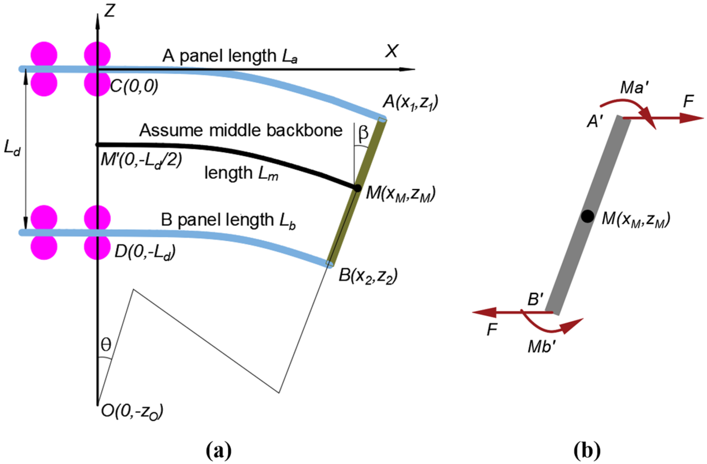
After the experiment, we wanted to delve into if a quasi-rigid model could be established. Upon comparison, one may notice that there is no centric backbone in our robot, as opposed to conventional continuum robots. For this reason, we assume a virtual backbone that runs through the middle axis of the two panels, as shown in
Figure 4a. Furthermore, by examining the moving platform in terms of internal forces, there is a pushing force at point A and a pulling force at point B, or vice versa, hence forces are always balanced but only with a moment, as shown in
Figure 4b. According to the Bernoulli–Euler beam theory, a beam with a pure-moment load will resemble a circular arc. This loading condition under a pure-moment scenario indicates that the middle backbone would bend into a circular shape. Therefore, we assume the shape of the middle axis (virtual backbone) is of an arc. Since the arc is perpendicular to the
Z axis at the start point, the center coordinate of the arc is 0 in
X direction and
in
Z direction. In other words, the middle backbone has the start point at
and the end point at
. Therefore, a circle equation can be written as
from which
zo can be determined for given
and
as
To this end, we have found the center of the circular arc of the middle axis of the robot. The next step is to determine the radius of the circle. This can be readily obtained by subtracting
zo by the half of the distance between the two panels, as shown in
Figure 4.
Based on the circle center, we can obtain the following relation
leading to the angle
θ as
Based on this angle, the arc length of the middle backbone can be determined as
Now let us look at the experiment data to draw certain useful relationships.
Table 2 shows the length of the middle backbone under different panel lengths. In this table,
represents the difference between the two panels. The initial lengths of the two panels were both at 0.15 m, and panel
A is pushed forward by 0.05 m for each increment. By using the previously mentioned 3D optical device, the end coordinates of the two panels were measured and the position of the moving platform
and
were calculated by using Equations (9) and (10). We further determined the center of the middle backbone and the radius by Equations (13) and (14), and angle
θ and the middle backbone length
by Equations (16) and (17).
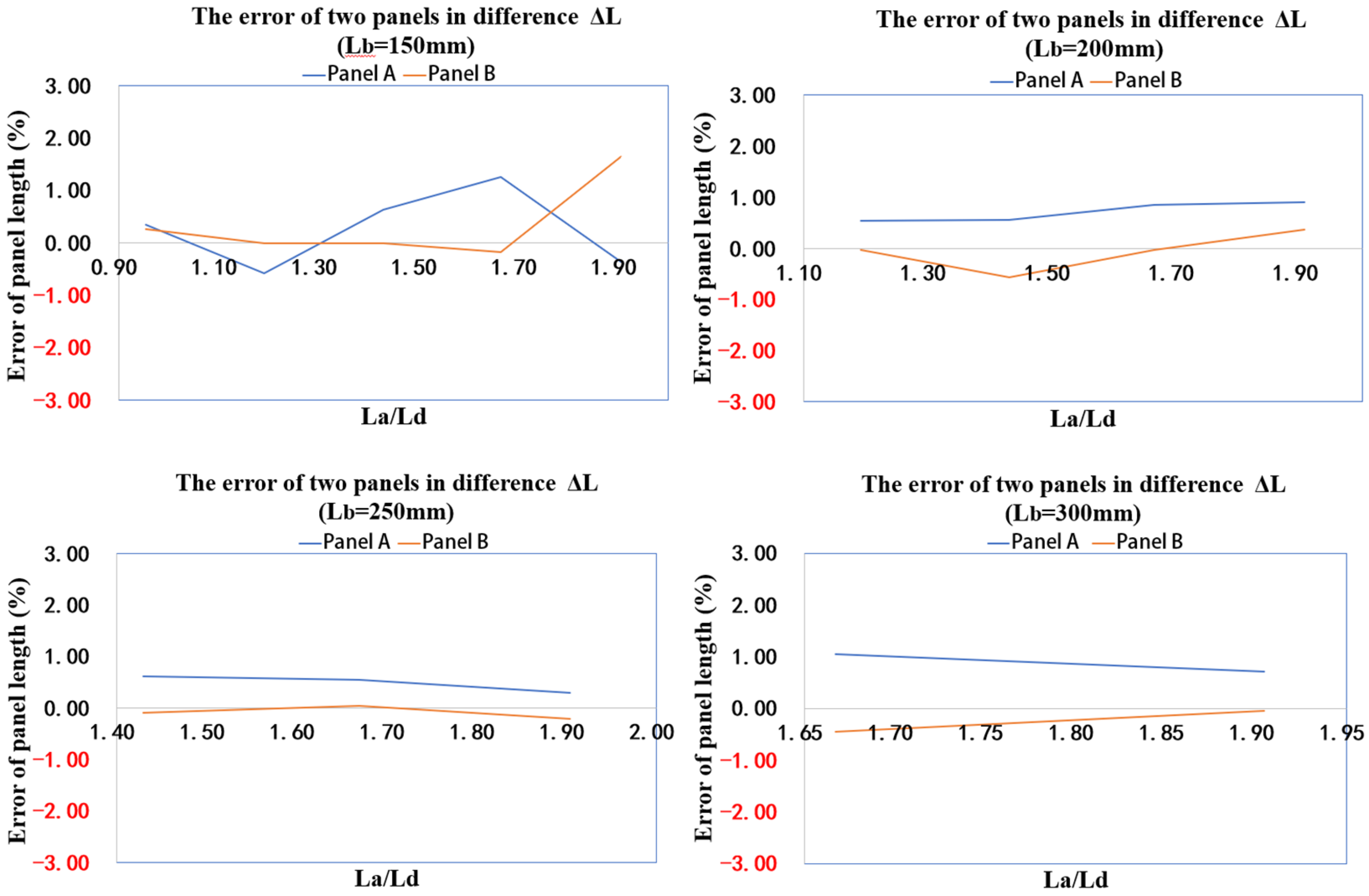
Table 3,
Table 4,
Table 5 and
Table 6 repeated the same experiments but with different start lengths of panel
B to cover the entire motion range for our study. According to Equations (13), (14), (16) and (17), the arc length of the middle backbone can be expressed in terms of
,
β and
as
The proposed inverse kinematics is based on the observation from
Table 2 to
Table 6. It can be found from these tables that
and
have very close values, from which the first approximate relation is obtained to relate the panel lengths to
Lm as
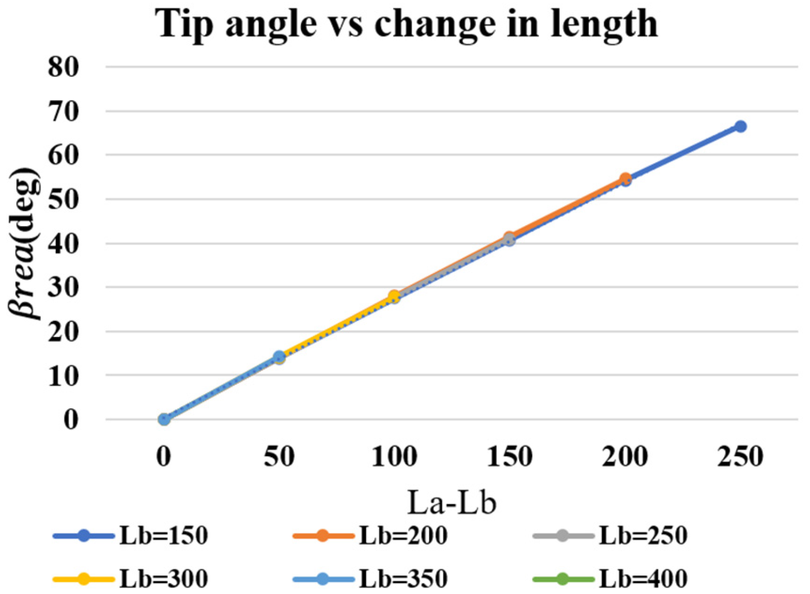
Furthermore,
Figure 5 is the experiment data of
Table 1 showing that the tip angle
β is linearly proportional to the length difference of the two panels
[
21], from which the second approximate relationship is obtained as
where
is the tip angle defined before and
k is the constant coefficient depending on the material of the two panels. From Equations (20) and (21), we can now solve the panel lengths as
To summarize, the inverse kinematic problem at hand can be solved by our proposed simplified approach as follows. For the given pose of the robot’s end-effector (moving platform), i.e., and β, Equation (19) is first used to determine Lm, and then Equation (22) and Equation (23) are used to determine the panel lengths and that will drive the robot to reach the given position and orientation angle β. Apparently, the proposed method provides an approximate closed-form solution that can be readily implemented for real-time applications. The only caveat is that k needs to be calibrated beforehand based on the panel material used.

 ,
, 


