Dynamic Tangential Contact Stiffness and Damping Model of the Solid–Liquid Interface

Abstract

In order to establish the tangential contact stiffness and damping model of the solid–liquid interface by tangential exciting vibration force under mixed lubrication, the finite difference method was firstly used to solve the average flow equation considering the effect of roughness on the lubrication effect, and the bearing capacity, shear force, and friction coefficient of the oil film were obtained, and thereby the dynamic tangential contact stiffness and damping of the oil film under tangential harmonic excitation were calculated. Then, according to the relationship between the normal deformation and the load of the solid contact microconvex body in the elastic/elastic–plastic/plastic deformation stage, integrating the tangential stick–slip theory, considering the effect of fluid lubrication on the solid contact friction coefficient, and tangential dynamic excitation, the tangential contact stiffness and damping of the microconvex body in three deformation stages were calculated. Furthermore, the dynamic tangential contact stiffness and damping of the solid–liquid interface were obtained by summing the solid surface contact part and the solid–liquid contact part in parallel according to the assumption of microconvex Gaussian distribution. Finally, through simulation analysis and experiments, the variation of the tangential dynamic contact stiffness and damping of the solid–liquid interface with normal load, tangential exciting frequency, and displacement amplitude was revealed and verified.

1. Introduction

In machine tools and other mechanical equipment, there exists a large number of interfaces between their parts. In order to reduce friction and wear, a lubricating medium usually exists between the interfaces, thus forming the solid–liquid interface. In different working conditions, the interface lies in different lubrication states, and usually several lubrication states exist at the same time, that is, a mixed-lubrication state. For example, gears, rolling bearings, cams, etc., at low speed, during start–stop, or under impact load are in the state of mixed elastohydrodynamic lubrication [1]; the linear-motion rolling guide pair in CNC machine tools is in a mixed-lubrication state when the slippage speed is 0.001~1 m/s [2]. The results of the research show that static and dynamic characteristics of mechanical systems, such as vibration and noise characteristics, fatigue and wear characteristics, contact pressure distribution, and working stability, are directly affected by the variation of contact stiffness and damping [3,4,5]. The contact state of the solid–liquid interface in the state of mixed lubrication is complex, so it is difficult to obtain the contact stiffness and damping parameters in actual operation. This is why the empirical values obtained in certain conditions are still used to replace [6,7,8] in the analysis and design of mechanical systems at home and abroad, but this empirical value is not universal. Therefore, to accurately obtain the joint contact stiffness and damping parameters under mixed lubrication, clarifying and revealing their influencing factors and laws is key to improving the performance of the whole machine in the process of mechanical equipment design and manufacturing.

In the study of contact characteristics of the solid–liquid interface, scholars use various experimental methods to directly measure stiffness or damping. Gonzalez-Valadez et al. [9] measured the normal stiffness of the solid–liquid interface under a static state using the ultrasonic reflection coefficient method. Dwyer-Joyce et al. [10] measured the normal contact stiffness of lubricating steel balls in states from static and mixed to full-film when slipping on the steel disk using the ultrasonic reflection method and found that with the increase in slippage speed, the contribution of liquid stiffness to the total stiffness gradually increased, and even became the main part, even in the static state. The liquid stiffness also contributed to the total stiffness. The stiffness ratio was determined using the mixed-lubrication model, and the lubricating film stiffness and the microconvex contact stiffness were separated from the measured combined stiffness, which solved the problem that it was difficult to measure under-boundary or mixed-film lubrication because of the high similarity between oil film thickness and surface roughness. Shi et al. [11] proposed an experimental method based on contact resonance to extract the normal contact stiffness and damping of the real rough surface under light load, and further studied the effect of the lubricant and abrasive wear on the contact stiffness and damping of the interface. Ren Peng et al. [12] used the peak resonance method to obtain the overall natural frequency of the slip guideway system and further calculate the equivalent normal dynamic stiffness of the dry friction and oil lubrication system. The simulation results showed that the increase in slippage speed reduced the dynamic stiffness of the joint. When the joint surface pressure was large or there was lubrication, the velocity had little effect on the dynamic stiffness. Although the stiffness or damping parameters of the solid–liquid interface can be obtained using various experimental methods, these methods require a large number of tests, and it is difficult to ensure reliability, ergodicity, and versatility [13].

Many researchers have also tried to establish the contact model of the solid–liquid interface directly using the fractal theory or the statistical theory. Patir and Cheng [14] established an average flow model considering the effect of rough surface microtopography on the contact characteristics of elastohydrodynamic lubrication and studied the relationship between surface topography and the lubrication state from a statistical point of view. Xiao Huifang et al. [15] established the normal stiffness model of solid contact using a statistical model, measured the liquid stiffness using the ultrasonic reflection coefficient method, and then coupled them to obtain the static normal stiffness of a mixed-lubrication bonding surface. It was concluded that the acoustic impedance of the lubricating medium is the main factor affecting the liquid contact stiffness. Sun et al. [16] derived the expression of liquid stiffness based on the ultrasonic spring model, the thin-film resonance model, and the Taylor approximate equation. The expression shows that liquid stiffness is only related to material properties and equivalent thickness. The equivalent deformation of an elastic rough surface was used to express the equivalent thickness of the lubricant, and a two-dimensional fractal model of static normal stiffness of a mixed-lubrication joint surface was established. Li Ling and Wen Xiaoyu et al. [17,18,19] used the three-dimensional fractal theory to characterize a rough surface, establish the contact stiffness model of the solid surface based on the statistical method, and establish the oil film stiffness model by determining the equivalent thickness of the oil film. As a result, the normal static contact stiffness of the joint under mixed lubrication was obtained. Most of the above studies focused on the normal static contact parameters.

Most of the above studies were on normal static contact parameters, and there are relatively few studies on tangential contact characteristics, but the research results of Changjiang Zhou [20,21] and others are worthy of attention as they provide good ideas for modeling the tangential contact stiffness and damping of the solid–liquid interface. In the literature [20], they equated the viscoelastic fluid in the straight cylindrical gear transmission to a massless spring unit, established the oil film’s normal stiffness model, and proposed the tangential stiffness model in fully flooded lubrication based on the assumption of equal shear stress on the surface of the laminar unit, while the contact surface stiffness and its effect on oil film stiffness were not included. Factually, the asperity contact had a significant influence on the oil film stiffness in mixed-lubrication contact.In the literature [21], innovative stiffness and damping models for oil films were proposed and developed to account for the impacts in both normal and tangential directions.The combined stiffness and damping consist of two parts: oil film and gear stiffness and damping. Drawing on this approach, the problem of modeling dynamic tangential contact parameters for face contact can be studied, and the effects of the contact microconvex body undergoing elastic/elastic–plastic/plastic deformation in the normal direction and the changes of parameters such as oil film thickness and load-carrying capacity on the tangential viscous and micro-slip states can be comprehensively considered.

Based on the GW [22] rough surface contact model and the Cattaneo–Mindlin [23,24,25] stick–slip theory, this paper takes the solid–liquid interface in the mixed-lubrication state as the research object and analyzes the elastic/elastic–plastic/plastic deformation of the contact microconvex body in normal direction and viscosity and micro-slip in the tangential direction under the action of normal static preload and tangential small vibration load. With the application of contact mechanics and statistics theory, the stiffness and damping of liquids and solids are obtained by solving the fluid Reynolds equation and the solid contact deformation equation, respectively, and the dynamic tangential contact stiffness and damping model of the solid–liquid interface is established. Through the model simulation, the effects of different normal loads, tangential excitation frequency, and relative displacement amplitude on the tangential dynamic contact stiffness and damping were analyzed, and the model was verified by means of experiments.

2. Calculation Model for Tangential Contact Stiffness and Damping of the Solid–Liquid Interface Fluid

According to the load distribution idea of a mixed-lubrication interface [15], the external load of the bonding surface is borne by both the fluid lubrication medium pressure and the solid microconvex contact force. Therefore, the total stiffness and damping of the solid–liquid interface under mixed lubrication were equal to the sum of the contact stiffness and damping of the solid microconvex body and the fluid lubricating medium, respectively.

The fluid part must start with the average flow equation considering the roughness lubrication effect and determine the oil film pressure distribution in order to further obtain the oil film shear force and then calculate the tangential stiffness and damping of the oil film.

2.1. Average Flow Equation Considering the Roughness Lubrication Effect

For the solid–liquid interface in the state of mixed lubrication, the average flow equation established by Patir and Cheng [14] that takes into account the effect of roughness on the lubrication effect is cited in Equation (1):

$$\begin{array}{l}\hspace{1em}\hspace{1em}\hspace{1em}\hspace{1em}\frac{\partial }{\partial x}\left(\frac{h_r^3}{{\eta }_f}{\varphi }_x\frac{\partial \overline{p_f}}{\partial x}\right)+\frac{\partial }{\partial y}\left(\frac{h_r^3}{{\eta }_f}{\varphi }_y\frac{\partial \overline{p_f}}{\partial y}\right)\\ \hspace{1em}\hspace{1em}\hspace{1em}\hspace{1em}\hspace{1em}\hspace{1em}\hspace{1em}\hspace{1em}\hspace{1em}\hspace{1em}=6\left[\left(U_0+U_{\mathrm{h}}\right)\frac{\partial \overline{h_r}}{\partial x}+\left(U_0-U_{\mathrm{h}}\right)\sigma \frac{\partial {\varphi }_s}{\partial x}+2\frac{\partial \overline{h_r}}{\partial t}\right]\end{array}$$

(1)

where the first item on the right is the dynamic pressure caused by rolling, the second is the dynamic pressure caused by slippage, and the third is the extrusion term. Among them, $\overline{p_f}$ is the average oil film pressure; $\overline{h_r}$ is the average actual oil film thickness at each point; $\sigma$ is the comprehensive root mean square of two rough surfaces, which is called comprehensive roughness; ϕ_x and ϕ_y are pressure flow factors in the direction of x and y, indicating the ratio of the average pressure flow between rough surfaces to that between smooth surfaces; ϕ_s is the pressure flow factor which takes into account the effect of pressure flow caused by the relative slippage of two rough surfaces; U₀, U_h, V₀, and V_h are, respectively, expressed as the relative slippage velocities of the two surfaces in the direction of X and Y; ${\eta }_f$ is the viscosity of lubricating oil, which is calculated using the Reoland viscosity–pressure relationship [26] as shown in Equation (2):

$$\begin{array}{cc}{\eta }_f={\eta }_{0}exp\left\{\left(ln{\eta }_0+9.67\right)\left[-1+{\left(1+\frac{p}{p_0}\right)}^z\right]\right\}& \hfill |\left(2-7\right)\end{array}$$

(2)

where ${\eta }_f$ is the viscosity at pressure p; η₀ is the viscosity at atmospheric pressure; p₀ is the pressure coefficient which can be indicated as $5.1\times {10}^{-9}$; for general mineral oil, z can usually be taken as 0.68.

It can be seen from Equation (1) that the oil film pressure at the solid–liquid interface is caused by two reasons: one is the hydrodynamic pressure caused by the mutual movement of the motion pair and the other is the extrusion pressure caused by the motion of the motion pair along the film thickness direction. The research object of this paper was the stiffness and damping under a tangential exciting load, and the normal load was static, so the extrusion term was ignored and the flow equation was further simplified.

In addition, according to [27], the general flow of a fluid in a narrow gap, pipe, or between two plates takes into account the wall non-slip condition (the velocity at the wall is zero), that is, the velocity when one fixed surface is fixed and the other surface considers a viscous condition. The fluid flow considered in this paper is the microflow caused by tangential vibration of the bonding surface, namely $U=X_0\omega cos\omega t$. The average flow equation solves the problem of full-film lubrication considering roughness, while this paper deals with mixed lubrication. With the change of load, the contact surface mostly had partial film lubrication. Therefore, Wu [28] and others introduced contact probability factor ϕ_c to improve the average flow model:

$$\frac{\partial }{\partial x}\left(\frac{h_r^3}{{\eta }_f}{\varphi }_x\frac{\partial \overline{p_f}}{\partial x}\right)+\frac{\partial }{\partial y}\left(\frac{h_r^3}{{\eta }_f}{\varphi }_y\frac{\partial \overline{p_f}}{\partial y}\right)=6U\left[{\varphi }_c\frac{\partial h}{\partial x}+\sigma \frac{\partial {\varphi }_s}{\partial x}\right]$$

(3)

where ${\varphi }_c=\frac{\partial {\overline{h}}_r}{\partial h}$, and when the surface roughness distribution characteristics are determined, the contact factor is only a function of the film thickness ratio $\lambda (\lambda =\frac{h_r}{\sigma })$, which reflects the proportion of the noncontact part of the lubricated surface; ϕ_x and ϕ_y are the pressure flow factors, ϕ_s is the shear flow factor. In order to facilitate the engineering application, the following fitting equation [26] is generally used to make the calculation:

$${\varphi }_x=\{\begin{array}{c}1-c_1{e}^{-c_2\lambda },\lambda \le 1\\ 1-c_1{e}^{-c_2},\lambda >1\end{array}$$

(4)

$${\varphi }_y\left(\lambda ,\gamma \right)={\varphi }_x\left(\lambda ,\raisebox{1ex}{$1$}\!\left/ \!\raisebox{-1ex}{$\lambda $}\right.\right)$$

(5)

$${\varphi }_s=\{\begin{array}{c}{A}_1{\lambda }^{{\alpha }_1}{e}^{-{\alpha }_2\lambda +{\alpha }_3{\lambda }^2},\lambda \le 5\\ A_2{e}^{-0.25\lambda },\lambda >5\end{array}$$

(6)

$${\varphi }_c=\{\begin{array}{c}\hfill e^{-0.6912+0.782\lambda -0.304{\lambda }^2+0.041{\lambda }^3},\lambda <3\hfill \\ \hfill 1 ,\lambda \ge 3\hfill \end{array}$$

(7)

where c₁, c₂, A₁, A₂, α₁, α₂, and α₃ are the parameters related to direction parameter γ, and the specific value can be obtained by referring to the relevant tables in reference [28].

At present, it is common to use the finite element method, the multigrid method, and the finite difference method to solve the flow equation, in which the finite difference method is characterized by mature algorithm, simple programming, and wide application to engineering. According to [16], under the static contact state of mixed lubrication, the thickness of the oil film can correspond to the equivalent deformation of a rough surface. Therefore, under a given normal load, the oil film thickness can be determined by calculating the rough surface deformation, and then the Reynolds equation is solved by means of the finite difference method to determine the oil film pressure.

Using $H=\frac{h_r}{h_0};P=\frac{\overline{p_f}}{p_0};X=\frac{x}{L};Y=\frac{y}{L};\eta =\frac{{\eta }_f}{{\eta }_0};{\psi }_1=\frac{6U{\eta }_{f}L}{h_0{}^2{p}_0};{\psi }_2=\frac{6U{\eta }_{f}L\sigma }{h_0{}^3{p}_0}$, among which h₀, p₀, ${\eta }_0$, and L are constants for reference, the dimensionless average Reynolds equation thus obtained is as follows:

$$\frac{\partial }{\partial X}\left({\varphi }_x{H}^3\frac{\partial P}{\partial X}\right)+\frac{\partial }{\partial Y}\left({\varphi }_y{H}^3\frac{\partial P}{\partial Y}\right)={\Psi }_2\frac{\partial {\varphi }_c}{\partial X}+{\Psi }_1{\varphi }_s\frac{\partial H}{\partial x}$$

(8)

The equally spaced meshing is carried out in the XOY plane of the solution domain. The number of nodes in the X and Y directions is m and n, and the distance between nodes is ΔX and ΔY, whose positions are represented as i and j. Using the five-point difference method [29] and references [26,30], the difference form of Equation (8) can be obtained as follows:

$$\begin{array}{c}\mathrm{A}\left(i,j\right)P\left(i,j\right)-B\left(i,j\right)P\left(i-1,j\right)-C\left(i,j\right)P\left(i+1,j\right)-D\left(i,j\right)P\left(i,j-1\right)\\ -E\left(i,j\right)P\left(i,j+1\right)=F\left(i,j\right)\end{array}$$

(9)

where

$$\begin{array}{c}B\left(i,j\right)=\frac{\left[{\varphi }_x\left(i-1,j\right)H^3\left(i-1,j\right)+{\varphi }_x\left(i,j\right)H^3\left(i,j\right)\right]}{2\Delta X^2}\\ C\left(i,j\right)=\frac{\left[{\varphi }_x\left(i+1,j\right)H^3\left(i+1,j\right)+{\varphi }_x\left(i,j\right)H^3\left(i,j\right)\right]}{2\Delta X^2}\\ D\left(i,j\right)=\frac{\left[{\varphi }_y\left(i,j-1\right)H^3\left(i,j-1\right)+{\varphi }_y\left(i,j\right)H^3\left(i,j\right)\right]}{2\Delta Y^2}\\ E\left(i,j\right)=\frac{\left[{\varphi }_y\left(i,j+1\right)H^3\left(i,j+1\right)+{\varphi }_y\left(i,j\right)H^3\left(i,j\right)\right]}{2\Delta Y^2}\\ A\left(i,j\right)=B\left(i,j\right)+C\left(i,j\right)+D\left(i,j\right)+E\left(i,j\right)\\ F\left(i,j\right)=\frac{{\psi }_2\left(i+j\right)}{2\mathsf{\Delta }X}\left[{\varphi }_c\left(i+1,j\right)-{\varphi }_c\left(i-1,j\right)\right]+\frac{{\psi }_1\left(i+j\right)}{2\mathsf{\Delta }X}{\varphi }_s\left(i,j\right)\left[H\left(i+1,j\right)-H\left(i-1,j\right)\right]\end{array}$$

In order to converge quickly, the relaxation iterative method is used to solve the difference equation.

$$P^{k+1}\left(i,j\right)=P^k\left(i,j\right)+\alpha ✶ \mathsf{\Delta }P\left(i,j\right)$$

(10)

where $\mathsf{\Delta }P\left(i,j\right)=P^{k+1}\left(i,j\right)-P^k\left(i,j\right)$

$$\begin{array}{c}{P}^{k+1}\left(i,j\right)=\\ \frac{\left[B\left(i,j\right)P^k\left(i-1,j\right)+C\left(i,j\right)P^k\left(i+1,j\right)+D\left(i,j\right)P^k\left(i,j-1\right)+E\left(i,j\right)P^k\left(i,j+1\right)\right]}{A\left(i,j\right)}=G\end{array}$$

Thus,

$$P^{k+1}\left(i,j\right)=\alpha ✶ G+\left(1-\alpha \right) ✶ P^k\left(i,j\right)$$

(11)

where α is the relaxation factor. According to the calculation experience, the overrelaxation iteration is adopted and $\alpha =1.95$ is taken.

In summary, according to the known parameters, the oil film pressure distribution can be obtained by dimensionless treatment and iterative solution.

2.2. Calculation of the Bearing Capacity of the Solid–Liquid Interface

The load on the solid–liquid interface under mixed lubrication is borne by the rough surface microconvex body and the oil film [15]. On the XOY plane, two areas’ length L and width W are taken, and the bearing capacity P₁ of the microconvex body is as follows:

$$P_1={{\displaystyle \int }}_0^W{{\displaystyle \int }}_0^L{P}_{ns}dxdy$$

(12)

where $P_{ns}$ is the pressure of the microconvex body, and the specific calculation is described in Section 3.3.

The bearing capacity of the oil film P₂ is as follows:

$$P_2={{\displaystyle \int }}_0^W{{\displaystyle \int }}_0^L\overline{p_f}dxdy$$

(13)

The total bearing capacity P is as follows:

$$P=P_1+P_2$$

(14)

2.3. Calculation of Viscous Shear Force of the Oil Film on the Solid–Liquid Interface

The shear force of the oil film is calculated by means of the model proposed by Patir and Cheng [14]:

$$F_f=-{{\displaystyle \int }}_0^W{{\displaystyle \int }}_0^L\left[\frac{{\eta }_{f}U}{h_r}\left({\varphi }_f+{\varphi }_{fs}\right)\right]dxdy$$

(15)

where ${\varphi }_f$ and ${\varphi }_{fs}$ are shear stress factors, and their numerical equations are represented as follows:

$${\varphi }_{fs}=A_3{\lambda }^{{\alpha }_4}\exp \left(-{\alpha }_5\lambda +{\alpha }_6{\lambda }^2\right)$$

(16)

$${\varphi }_f=\{\begin{array}{c}\frac{35}{32}\zeta \left\{\begin{array}{c}{\left(1-{\zeta }^2\right)}^3\ln \left[300\left(\zeta +1\right)\right]+\frac{1}{60}[-55+\\ \zeta \left(132+\zeta \left(345+\zeta \left(-160+\zeta \left(-405+\zeta \left(60+147\zeta \right)\right)\right)\right)\right)]\end{array}\right\},\lambda \le 3\\ \frac{35}{32}\zeta \left\{{\left(1-{\zeta }^2\right)}^{3}ln\frac{\zeta +1}{\zeta -1}+\frac{\zeta }{15}\left[66+{\zeta }^2\left(30{\zeta }^2-80\right)\right]\right\},\lambda >3\end{array}$$

(17)

where A₃, α₄, α_5, and α₆ are parameters related to the direction parameter γ, and their values can be found in [14], ζ = λ/3.

2.4. Calculation of the Friction Coefficient of the Solid–Liquid Interface

The total friction force of the solid–liquid interface consists of two parts: the shear force caused by the contact of the microconvex bodies on the two rough surfaces and the oil film shear force:

$$\mathrm{F}=-{{\displaystyle \int }}_0^W{{\displaystyle \int }}_0^L\left[\frac{{\eta }_{f}U}{h_r}\left({\varphi }_f+{\varphi }_{fs}\right) + {\mu }_s{P}_{rs}\right]dxdy$$

(18)

where ${\mu }_s$ is the coefficient of contact friction between two rough surfaces.

The friction coefficient $\mu$ of the solid–liquid interface is as follows:

$$\mu =\frac{F}{P}$$

(19)

2.5. Difference Model for Calculating Partial Tangential Stiffness and Damping of the Solid–Liquid Interface

When the tangential exciting load is applied to the solid–liquid interface, the stiffness and damping of the oil film are shown in small disturbance, resulting in displacement disturbance and velocity disturbance, and the shear force of the oil film changes. Therefore, the finite difference method is used to determine the dynamic stiffness and damping of the oil film on the solid–liquid interface. According to [31], the relationship between the oil film disturbance force and stiffness, damping, and displacement velocity is as follows:

$$\mathsf{\Delta }{F}_{\tau }=k_{\tau }\mathsf{\Delta }x+c_{\tau }{x}^{\prime }=\mathsf{\Delta }{F}_{\tau d}+\mathsf{\Delta }{F}_{\tau v}$$

(20)

where $\mathsf{\Delta }{F}_{\tau }$ is the change in the shear force of the oil film, $k_{\tau }$ is the stiffness, $c_{\tau }$ is the damping, $\mathsf{\Delta }x$ is the disturbance displacement (that is, the dynamic displacement caused by tangential excitation), $x^{\prime }$ is the disturbance velocity (that is, the tangential simple harmonic excitation velocity), $\mathsf{\Delta }{F}_{\tau d}$ is the change of the oil film force caused by displacement disturbance, and $\mathsf{\Delta }{F}_{\tau v}$ is the velocity disturbance that causes the change of the oil film force. Therefore, the oil film stiffness and damping caused by tangential excitation displacement disturbance are as follows:

$$\{\begin{array}{c}{k}_{\tau }=\frac{\Delta F_{\tau d}}{\Delta x}\\ c_{\tau }=\frac{\Delta F_{\tau v}}{\Delta x^{\prime }}\end{array}$$

(21)

Three problems need to be solved in the calculation of the above equations: (1) to calculate the shear force of the oil film which changes before and after a certain time caused by displacement and velocity, that is, the instantaneous value of Equation (14); (2) the solid–liquid interface is affected by the external load and tangential excitation, and the extrusion deformation of the oil film network needs to be updated by means of the difference method; and (3) to calculate the stiffness and damping, it is necessary to calculate the displacement disturbance and the velocity disturbance, as well asthe stiffness and damping through the ratio of the oil film force to the disturbance displacement and the velocity caused by the disturbance.

The small perturbation method is used to determine the oil film stiffness and damping of the finite difference method at each time t (t ∈ [0, T], t = T/N, T is a period, N is the number of difference points):

$$\{\begin{array}{c}{K}_{\tau f}^{\left(t\right)}=k_{\tau }=\frac{\Delta F_{\tau d}}{\Delta x}=\frac{F_{\tau d}^{\prime }-F_{\tau d}}{\Delta x}\\ C_{\tau f}^{\left(t\right)}=c_{\tau }=\frac{\Delta F_{\tau v}}{\Delta x^{\prime }}=\frac{F_{\tau v}^{\prime }-F_{\tau v}}{\Delta x^{\prime }}\end{array}$$

(22)

where $F_{\tau d}^{\prime }$ and $F_{\tau v}^{\prime }$ are the transient oil film forces caused by the displacement and velocity disturbance at the previous moment, respectively, while $F_{\tau d}$ and $F_{\tau v}$ are the transient oil film forces at the current moment, and the transient oil film force here is the viscous shear force of the oil film obtained by Equation (15), the numerical method for x is $\Delta x_i={{\displaystyle \int }}_{t_{i-1}}^{t_i}{X}_0\omega \cos \omega tdt$, and the numerical method for $\Delta x^{\prime }$ is $\Delta x_i{}^{\prime }=X_0\omega \left(\cos \omega t_i-\cos \omega t_{i-1}\right)$.

The average stiffness ${\overline{K}}_{\tau f}$ and damping ${\overline{C}}_{\tau f}$ of the tangential oil film in one vibration period are determined as follows:

$$\{\begin{array}{l}\overline{K_{\tau f}}=\frac{{\displaystyle \sum {}_{t=0}^{\frac{T}{2}}{K}_{\tau f}^{(t)}+{\displaystyle \sum {}_{t=\frac{T}{2}}^T{K}_{\tau f}^{(t)}}}}{T}\\ \overline{C_{\tau f}}=\frac{{\displaystyle \sum {}_{t=0}^{\frac{T}{2}}{C}_{\tau f}^{(t)}+{\displaystyle \sum {}_{t=\frac{T}{2}}^T{C}_{\tau f}^{(t)}}}}{T}\end{array}$$

(23)

The computer program implementation of the above process is shown in Figure 1.

3. Calculation Model of Tangential Contact Stiffness and Damping of the Solid–Liquid Interface

Based on the GW [22] contact model assumption, the solid–solid interface is equivalent to the contact between a rough surface and a smooth rigid plane, as shown in Figure 2, where h is the distance between the rigid smooth plane and the surface average height line, z is the height of the microconvex body on the joint surface, which obeys the Gaussian distribution, d is the distance between the rigid smooth plane and the microconvex average height line, y_s is the distance between the microconvex average height line and the surface average height line, R is the peak curvature radius of the microconvex, and the normal deformation of the microconvex body is $\delta =z-d$. The equivalent rough surface parameters are as follows: elastic modulus E, shear modulus G, Poisson’s ratio v, mean square deviation σ, area density of microconvex body ρ, rough surface topography parameter $\beta =\sigma R\rho$.

The contact model of the microconvex body is shown in Figure 3: P_n is the normal force, and the deformation caused is δ; $P_{\tau }$ is the tangential force, including preload and small harmonic vibration load; tangential displacement ${\xi }_0$ is caused by the preload, tangential dynamic displacement caused by the harmonic vibration load is $△\xi =X_0\sin \omega t$, where X₀ is the amplitude of tangential dynamic displacement of the bonding plane, $\omega$ is the vibration circle frequency, and the total displacement of the microconvex body is $\xi ={\xi }_0+△\xi$.

According to the Cattaneo–Mindlin [23,24] model, under a normal load, the microconvex body forms a circular contact area with a radius of r, and the contact compressive stress distribution is uneven. As shown in Figure 3, the microconvex body under goes elastic, elastic–plastic, and plastic deformation. At the same time, under the action of a tangential load, the local micro-slip of the bonding surface occurs, forming a stick area with a radius of $c(c=r\left(1-\frac{P_{\tau }}{\mu P_n}{)}^{\frac{1}{3}}\right)$ and a micro-slip zone with a radius of r – c. When there is no tangential load, the viscous area occupies the whole contact surface. In the process of the tangential load increasing gradually, the micro-slip zone expands from the contact edge to the center area to the whole contact surface. When the tangential load reaches $\mu P_n$, the micro-slip zone occupies the whole contact surface, and then the microconvex body moves macroscopically. The beginning and development of the micro-slip body must have an important influence on the later macromovement, so this paper studies the contact characteristics of the microconvex body in the viscous static state and the micro-slip dynamic state.

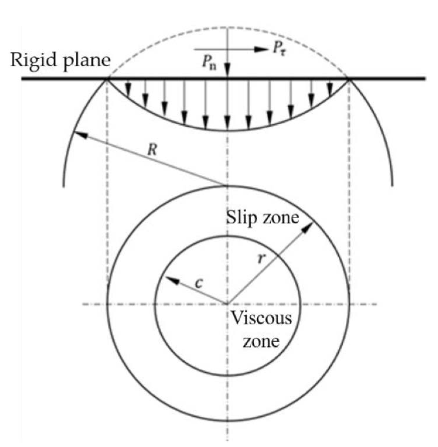
3.1. Relationship between a Normal Load and Deformation of the Microconvex Body

Under a normal load, the microconvex body undergoes elastic, elastic–plastic, and plastic deformation in turn. The normal contact loads of these three stages are P_ne, P_nep, and P_np, respectively. The relationship between them and the amount of deformation $\delta$[32,33,34,35] are as follows:

$$P_{ne}=\frac{4}{3}E{R}^{\frac{1}{2}}{\delta }^{\frac{3}{2}},\delta <{\delta }_e$$

(24)

$$P_{nep}=\frac{4}{3}E{R}^{\frac{1}{2}}{\delta }_e{}^{\frac{3}{2}}\left[1.32{\left(\frac{\delta }{{\delta }_e}-1\right)}^{1.27}+1\right],{\delta }_e<\delta <110{\delta }_e$$

(25)

$$P_{np}=2\pi RH\delta ,\delta >110{\delta }_e$$

(26)

where ${\delta }_e$ is the critical deformation of the microconvex body that transitions from the elastic deformation state to the elastic–plastic deformation state [36]:

$${\delta }_e={\left(\frac{3\pi kH}{4E}\right)}^{2}R$$

(27)

where k is the critical yield stress coefficient, $k=1.295\exp \left(0.736\nu \right)$, H is the yield stress of softer materials, and $\nu$ is Poisson’s ratio of softer materials.

3.2. Tangential Contact Stiffness and Damping Model of the Microconvex Body

To establish the tangential contact stiffness and damping model of the microconvex body, it is necessary to analyze and establish the relationship between the tangential load and the tangential displacement from the normal elastic/elastic–plastic/plastic deformation stage of the microconvex body and the various combined states of tangential viscosity and the micro-slip state.

3.2.1. Elastic Stage

When the tangential vibration load reaches the maximum static friction $\mu P_{ne}$, the microconvex body transitions from the viscous state in the elastic deformation stage to the micro-slip state. According to the Mindlin theory [26], the relationship between the tangential load and the tangential displacement is as follows:

$$P_{\tau e}=\{\begin{array}{c}\mu P_{ne}\left[1-{\left(1-\frac{\xi }{{\xi }_e}\right)}^{\frac{3}{2}}\right],\xi \le {\xi }_e\\ \mu P_{ne},\xi >{\xi }_e\end{array}$$

(28)

where ${\xi }_e$ is the critical displacement of the microconvex body from the viscous state to the micro-slip state in the stage of elastic deformation, ${\xi }_e=\frac{\mu E\left(2-\nu \right)\delta }{4G}$.

According to the hysteresis criterion in [37], that is, the relationship between the load and the deformation in the process of loading/unloading, the contact characteristic parameters of the microconvex body in the stage of elastic deformation can be obtained.

(1) Viscous state in the elastic stage:

The relationships between tangential load $P_{\tau e\_st\_l}/P_{\tau e\_st\_d}$, stiffness $P_{\tau e\_st\_l}/P_{\tau e\_st\_d}$, and tangential displacement ξ in viscous state in the elastic stage are as follows:

$$P_{\tau e\_st}=\{\begin{array}{c}\frac{4}{3}\mu E{R}^{\frac{1}{2}}{\delta }^{\frac{3}{2}}\left[1-{\left(1-\frac{\xi }{{\xi }_e}\right)}^{\frac{3}{2}}\right] \mathrm{loading} P_{\tau e\_st\_l}\\ P_{\tau e\_m}-2P_{\tau e}\left(\frac{{\xi }_{e\_m}-\xi }{2}\right) \mathrm{unloading} P_{\tau e\_st\_d}\end{array}$$

(29)

$$k_{\tau e\_st\_l}=\frac{d{P}_{\tau e\_st\_l}}{d\xi }=\frac{2\sqrt{R}{\delta }^{\frac{3}{2}}\mu \sqrt{1-\frac{\xi }{{\xi }_e}}}{{\xi }_e}$$

(30)

$$k_{\tau e\_st\_d}=\frac{d{P}_{\tau e\_st\_d}}{d\xi }=\frac{4}{3}\sqrt{R}{\delta }^{\frac{3}{2}}E\mu \left[1-{\left(1-\frac{\xi }{{\xi }_e}\right)}^{\frac{2}{3}}\right]-\frac{8\sqrt{R}{\delta }^{\frac{3}{2}}E\mu \left(-\xi +{\xi }_{e\_m}\right)}{9{\xi }_e{\left(1-\frac{\xi }{{\xi }_e}\right)}^{\frac{1}{3}}}$$

(31)

In the loading/unloading process of the viscous state, energy dissipation $E_{\tau e\_st}$ in the elastic stage is as follows:

$$E_{\tau e\_st}={{\displaystyle \int }}_{-{\xi }_{e\_m}}^{{\xi }_{e\_m}}\left(P_{\tau e\_st\_l}-P_{\tau e\_st\_d}\right)d\xi$$

(32)

where $P_{\tau e\_m}$ is the tangential maximum force of the hysteresis curve when the microconvex body is in the elastic deformation phase and ${\xi }_{e\_m}$ is the maximum tangential displacement corresponding to the tangential maximum force.

(2) Micro-slip state in the elastic stage:

The relationships between tangential load $P_{\tau e\_sl\_l}/P_{\tau e\_sl\_d}$ and tangential displacement ξ in micro-slip state in the elastic stage are as follows:

$$P_{\tau e\_sl}=\{\begin{array}{c}\frac{4}{3}\mu E\sqrt{R}{\delta }^{\frac{3}{2}} \mathrm{loading} P_{\tau e\_sl\_l}\\ -\frac{4}{3}\mu E\sqrt{R}{\delta }^{\frac{3}{2}} \mathrm{unloading} P_{\tau e\_sl\_d}\end{array}$$

(33)

Thus, it can be seen that tangential load is only a function of the normal deformation and has nothing to do with tangential displacement, so the tangential contact stiffness $k_{\tau e\_sl\_l}/k_{\tau e\_sl\_d}$ are zero.

In the process of loading/unloading in the elastic micro-slip state, the energy dissipation $E_{\tau e\_sl}$ consists of two parts: the energy dissipation of the stick microconvex body and the energy dissipation of the micro-slip microconvex body. The energy dissipation in the loading/unloading process of the elastic–plastic/plastic micro-slip state discussed later is also composed of these two parts:

$$E_{\tau e\_\mathrm{sl}}={{\displaystyle \int }}_{-{\xi }_e}^{{\xi }_e}\left(P_{\tau e\_st\_l}-P_{\tau e\_st\_d}\right)d\xi +{{\displaystyle \int }}_{-{\xi }_{e\_m}+{\xi }_e}^{{\xi }_{e\_m}-{\xi }_e}\left(P_{\tau e\_sl\_l}-P_{\tau e\_sl\_d}\right)d\xi$$

(34)

3.2.2. Elastic–Plastic Stage

When the tangential vibration load reaches the maximum static friction $\mu P_{nep}$, the microconvex body transitions from the viscous state to the micro-slip state in the stage of elastic–plastic deformation. According to Mindlin and Fojimoto’s [34] theory, as well as [35,38,39,40,41], under the action of a normal load, the microconvex body forms a circular contact area with a radius of r $\left(r={(\frac{3R{P}_{nep}}{4E})}^{\frac{1}{3}}\right)$, and the distribution of normal compressive stress p(a) in this area is uneven, which is $\frac{3P_{nep}}{2\pi a^2}{\left[1-{(\frac{a}{r})}^2\right]}^{\frac{1}{2}}$. When the yield stress of the contact surface material is $p_y$, the microconvex body deforms in the radius of the $a\in (0,a_p)(a_p{}^2=r^2-\left(\frac{\pi R{p}_y}{2E}{)}^2\right)$ region, and the normal contact force P₂ in this region is constant, $P_2=\pi a_p{}^2{p}_y$. The elastic deformation of the microconvex body occurs in the radius of the $a\in (a_p,a)$ region, and its normal contact force is $P_1=2\pi {{\displaystyle \int }}_{a_p}^{a}p\left(r\right)rdr$. Therefore, the relationship between the tangential contact load and the tangential displacement is as follows:

$$P_{\tau ep}=\{\begin{array}{c}\mu P_1[1-\left(1-\frac{\xi }{{\xi }_{eep}}{)}^{\frac{3}{2}}\right]+\frac{\mu P_2\xi }{{\xi }_{pep}}\hfill \\ \mu P_{nep},\xi >{\xi }_{eep}\hfill \end{array},\xi \le {\xi }_{eep}$$

(35)

where ${\xi }_{pep}=\frac{{\mu }_1}{2G}{(\frac{H}{\pi })}^{\frac{1}{2}}{P}_2{}^{\frac{1}{2}}$,${\xi }_{eep}$ is the critical tangential relative displacement of the transition of the microconvex body from the viscous state to the micro-slip state in the stage of elastic–plastic deformation, ${\xi }_{eep}=\frac{3\left(2-\nu \right)\mu P_1}{16Gr}$.

According to the hysteresis criterion in [37], the contact characteristic parameters in the viscous and micro-slip states of the loading/unloading process in the elastic–plastic stage can be obtained.

(1) Viscous state in the elastic–plastic stage:

The relationship between tangential load $P_{\tau ep\_st\_l}/P_{\tau ep\_st\_d}$, stiffness $k_{\tau ep\_st\_l}/k_{\tau ep\_st\_d}$ and tangential displacement $\xi$ in the viscous state in the elastic–plastic stage are as follows:

$$P_{\tau ep\_st}=\{\begin{array}{c}\mu P_1\left[1-{\left(1-\frac{\xi }{{\xi }_{eep}}\right)}^{\frac{3}{2}}\right]+\frac{\mu P_2\xi }{{\xi }_{pep}} \mathrm{loading} p_{\tau ep\_st\_l}\\ P_{\tau ep\_m}-2P_{\tau ep}\left(\frac{{\xi }_{ep\_m}-\xi }{2}\right) \mathrm{unloading} p_{\tau ep\_st\_d}\end{array}$$

(36)

$$k_{\tau ep\_st\_l}=\frac{d{P}_{\tau ep\_st\_l}}{d\xi }=\frac{8Gr}{2-\nu }\sqrt{1-\frac{\xi }{{\xi }_{eep}}}+\frac{2}{3}G\sqrt{P_2}\sqrt{\frac{\pi }{H}}$$

(37)

$$\begin{array}{c}{k}_{\tau ep\_st\_d}=\frac{d{P}_{\tau ep\_st\_d}}{d\xi }=\mu P_1\left[1-{(1-\frac{\xi }{{\xi }_{eep}})}^{\frac{3}{2}}\right]\\ +\left(\xi -{\xi }_{ep\_m}\right)\left[\frac{8Gr}{2-\nu }\sqrt{1-\frac{\xi }{{\xi }_{eep}}}+\frac{2}{3}G\sqrt{\frac{\pi P_2}{H}}\right]+\frac{2}{3}G\xi \sqrt{\frac{\pi P_2}{H}}\end{array}$$

(38)

Energy dissipation during the loading and unloading in the elastic–plastic viscous state E_{τep_st} is as follows:

$$E_{\tau ep\_st}={{\displaystyle \int }}_{-{\xi }_{ep\_m}}^{{\xi }_{ep\_m}}\left(P_{\tau ep\_st\_l}-P_{\tau ep\_st\_d}\right)d\xi$$

(39)

(2) Micro-slip state in the elastic–plastic stage:

In the micro-slip state of the loading/unloading process in the elastic–plastic stage, the relationships between tangential load $P_{\tau ep\_sl\_l}/P_{\tau ep\_sl\_d}$ and tangential displacement $\xi$ are as follows:

$$P_{\tau ep\_sl}=\{\begin{array}{c}\frac{4}{3}\mu E{R}^{\frac{1}{2}}{\delta }_e{}^{\frac{3}{2}}\left[1.32{\left(\frac{\delta }{{\delta }_e}-1\right)}^{1.27}+1\right] \mathrm{loading} \left(P_{\tau ep\_sl\_l}\right)\\ -\frac{4}{3}\mu E{R}^{\frac{1}{2}}{\delta }_e{}^{\frac{3}{2}}\left[1.32{\left(\frac{\delta }{{\delta }_e}-1\right)}^{1.27}+1\right] \mathrm{unloading} \left(P_{\tau ep\_sl\_d}\right)\end{array}$$

(40)

Thus, it can be seen that tangential load is only a function of normal deformation and has nothing to do with tangential displacement, so the tangential contact stiffness $k_{\tau ep\_sl\_l}/k_{\tau ep\_sl\_d}$ are zero.

In the process of loading/unloading in the elastic micro-slip state, the energy dissipation $E_{\tau ep\_sl}$ consists of two parts: the energy dissipation of the stick microconvex body and the energy dissipation of the micro-slip microconvex body. The energy dissipation in the loading/unloading process of the elastic–plastic/plastic micro-slip state discussed later is also composed of these two parts:

$$E_{\tau ep\_sl}={{\displaystyle \int }}_{-{\xi }_{ep}}^{{\xi }_{ep}}\left(P_{\tau ep\_st\_l}-P_{\tau ep\_st\_d}\right)d\xi +{{\displaystyle \int }}_{-{\xi }_{ep\_m}+{\xi }_{ep}}^{{\xi }_{ep\_m}-{\xi }_{ep}}\left(P_{\tau ep\_sl\_l}-P_{\tau ep\_sl\_d}\right)d\xi$$

(41)

3.2.3. Plastic Stage

When the tangential vibration load exceeds the maximum static friction $\mu P_{np}$, the microconvex body transitions from the viscous state to the micro-slip state. The relationship between tangential load $P_{\tau p}$ and tangential displacement is as follows:

$$P_{\tau p}=\{\begin{array}{c}\frac{\mu P_{np}\xi }{{\xi }_p},\xi \le {\xi }_p\\ \mu P_{np},\xi >{\xi }_p\end{array}$$

(42)

where it is the critical displacement of the microconvex body from the viscous state to the micro-slip state in the stage of plastic deformation.

According to the hysteresis criterion in [37], the parameters related to the contact characteristics of the loading/unloading process in the complete plastic stage can be obtained.

(1) Viscous state in the plastic stage:

In the viscous state of the plastic stage, the relationship between tangential load $P_{\tau p\_st\_l}/P_{\tau p\_st\_d}$, stiffness $k_{\tau p\_st\_l}/k_{\tau p\_st\_d}$, and tangential displacement is as follows:

$$P_{\tau p\_st}=\{\begin{array}{c}{P}_{\tau p}\frac{\xi }{{\xi }_p} \mathrm{lloading} (P_{\tau p\_st\_l})\\ P_{\tau p\_m}-2P_{\tau p}\left(\frac{{\xi }_{p\_m}-\xi }{2}\right) \mathrm{unloading} (P_{\tau p\_st\_d}) \end{array}$$

(43)

$$k_{\tau p\_st\_l}=\frac{d{P}_{\tau p\_\mathrm{st}\_l}}{d\xi }=2\sqrt{2}\pi G\sqrt{R\delta }$$

(44)

In the unloading stage, the microconvex body is in plastic deformation, so the tangential contact stiffness $k_{\tau p\_st\_d}$ is ignored.

Energy dissipation $E_{\tau p\_st}$ during loading and unloading in the plastic viscous state:

$$E_{\tau p\_st}={{\displaystyle \int }}_{-{\xi }_{p\_m}}^{{\xi }_{p\_m}}\left(P_{\tau p\_st\_l}-P_{\tau p\_st\_d}\right)d\xi$$

(45)

(2) Micro-slip state in the plastic stage:

Tangential load $P_{\tau p\_sl\_l}/P_{\tau p\_sl\_d}$ and stiffness $k_{\tau p\_sl\_l}/k_{\tau p\_sl\_d}$ of the loading/unloading process in the fully plastic stage under the micro-slip state are as follows:

$$P_{\tau p\_sl}=\{\begin{array}{c}2\pi \mu RH\delta \mathrm{loading} \left(P_{\tau p\_sl\_l}\right)\\ -2\pi \mu RH\delta \mathrm{unloading} \left(P_{\tau p\_sl\_d}\right)\end{array}$$

(46)

Because tangential load is only a function of normal deformation and has nothing to do with tangential displacement, its contact stiffness is zero.

Energy dissipation $E_{\tau p\_sl}$ in the process of loading and unloading in the elastic–plastic micro-slip state:

$$E_{\tau p\_sl}={{\displaystyle \int }}_{-{\xi }_{p\_m}}^{{\xi }_{p\_m}}\left(P_{\tau p\_sl\_l}-P_{\tau p\_sl\_d}\right)d\xi$$

(47)

3.3. Dynamic Statistical Model of the Tangential Contact of Solids in the Solid–Iquid Interface

Based on the statistical theory, the contact characteristic parameter model of the above single microconvex body is extended to the whole solid interface. Let the nominal contact area of the joint be A_n, the number of microconvex bodies in this area be n, and the Gaussian distribution function of microconvex height be $\varphi \left(z\right)$, then the normal contact load of the solid is as follows:

$$\begin{array}{c}{P}_{ns}=n\left(P_{ne}+P_{nep}+P_{np}\right)\\ =\frac{4}{3}E\rho A_n{R}^{\frac{1}{2}}{{\displaystyle \int }}_d^{d+{\delta }_e}{\delta }^{\frac{3}{2}}\varphi \left(z\right)dz\\ +\frac{4}{3}E\rho A_n{R}^{\frac{1}{2}}{\delta }_e{}^{\frac{3}{2}}{{\displaystyle \int }}_{d+{\delta }_e}^{d+110{\delta }_e}\left[1.32{\left(\frac{\delta }{{\delta }_e}-1\right)}^{1.27}+1\right]\varphi \left(z\right)dz\\ +2\pi RH\rho A_n{{\displaystyle \int }}_{d+110{\delta }_e}^{+\infty }\delta \varphi \left(z\right)dz\end{array}$$

(48)

The total stiffness $K_{\tau \_l}$ of a solid under tangential contact loading is as follows:

$$\begin{array}{c}{K}_{\tau \_l}=n\left(k_{\tau e\_st\_l}+k_{\tau ep\_st\_l}+k_{\tau p\_st\_l}+k_{\tau e\_sd\_l}+k_{\tau ep\_sd\_l}+k_{\tau p\_sd\_l}\right)\\ =\rho A_n{{\displaystyle \int }}_d^{d+{\delta }_e}\frac{2\sqrt{R}{\delta }^{\frac{3}{2}}\mu \sqrt{1-\frac{\xi }{{\xi }_e}}}{{\xi }_e}\varphi \left(z\right)dz\\ +\rho A_n{{\displaystyle \int }}_{d+{\delta }_e}^{d+110{\delta }_e}\left[\frac{8Gr}{2-\nu }\sqrt{1-\frac{\xi }{{\xi }_{eep}}}+\frac{2}{3}G\sqrt{P_2}\sqrt{\frac{\pi }{H}}\right]\varphi \left(z\right)dz\\ +\rho A_n{{\displaystyle \int }}_{d+110{\delta }_e}^{\infty }2\sqrt{2}\pi G\sqrt{R\delta }\varphi \left(z\right)dz\end{array}$$

(49)

The total stiffness $K_{\tau \_d}$ of a solid’s tangential contact unloading is as follows:

$$\begin{array}{c}{K}_{\tau \_d}=n\left(k_{\tau e\_st\_d}+k_{\tau ep\_st\_d}+k_{\tau p\_st\_d}+k_{\tau e\_sd\_d}+k_{\tau ep\_sd\_d}+k_{\tau p\_sd\_d}\right)\\ =\rho A_n{{\displaystyle \int }}_d^{d+{\delta }_e}\frac{4}{3}\sqrt{R}{\delta }^{\frac{3}{2}}E\mu \left[1-{\left(1-\frac{\xi }{{\xi }_e}\right)}^{\frac{2}{3}}\right]-\frac{8\sqrt{R}{\delta }^{\frac{3}{2}}E\mu \left(-\xi +{\xi }_{e\_m}\right)}{9{\xi }_e{\left(1-\frac{\xi }{{\xi }_e}\right)}^{\frac{1}{3}}}\varphi \left(z\right)dz\\ +\rho A_n{{\displaystyle \int }}_{d+{\delta }_e}^{d+110{\delta }_e}\left\{\begin{array}{c}\mu P_1\left[1-{\left(1-\frac{\xi }{{\xi }_{eep}}\right)}^{\frac{3}{2}}\right]+\frac{2}{3}G\xi \sqrt{P_2}\sqrt{\frac{\pi }{H}}\\ +\left(\xi -{\xi }_{ep\_m}\right)\left[\frac{8Gr}{2-\nu }\sqrt{1-\frac{\xi }{{\xi }_{eep}}}+\frac{2}{3}G\sqrt{P_2}\sqrt{\frac{\pi }{H}}\right]\end{array}\right\}\varphi \left(z\right)dz\end{array}$$

(50)

Because $\xi ={\xi }_0+X_{0}sin\omega t$ is a dynamic variable regarding time t, the stiffness and damping parameters are also dynamic. From the point of view of analysis and application, this paper only focuses on the average value in one cycle. Therefore, dynamic tangential solid contact stiffness $K_{\tau s}$ is the average stiffness in a loading/unloading period T, that is,

$$K_{\tau s}=\frac{1}{T}\left({{\displaystyle \int }}_0^{\frac{T}{2}}{K}_{\tau \_l}dt+{{\displaystyle \int }}_{\frac{T}{2}}^{\mathrm{T}}{K}_{\tau \_d}dt\right)$$

(51)

where T is $\left(2k\pi -\frac{\pi }{2},2k\pi +\frac{3\pi }{2}\right), k\in N$. Using Equations (49) and (50) in this equation, we can obtain what is required.

According to the viscous equivalent damping principle [40], the equivalent viscous damping coefficient C of the solid contact part is

$$C=\frac{E}{\pi \omega X^2}$$

(52)

where E is the energy dissipated in a loading/unloading cycle, which is obtained from the sum of the tangential contact dissipative energy of the microconvex body in the elastic/elastic–plastic/plastic stage during the loading/unloading process:

$$\begin{array}{l}E=\rho A_n{\displaystyle {\int }_d^{d+{\delta }_e}(E_{\tau e\_st}+E_{\tau e\_sl})}\varphi (z)dz\\ +\rho A_n{\displaystyle {\int }_{d+{\delta }_e}^{d+110{\delta }_e}(E_{\tau ep\_st}+E_{\tau ep\_sl})\varphi (z)dz}\\ +\rho A_n{\displaystyle {\int }_{d+110{\delta }_e}^{\infty }(E_{\tau p\_st}+E_{\tau p\_sl})\varphi (z)dz}\end{array}$$

(53)

Use of Equations (32), (34), (39), (41), (45), and (47) in this Equation (53) yields what is required.

3.4. Calculation Model of Tangential Contact Stiffness and Damping of the Solid–Liquid Interface

The total stiffness of the solid–liquid interface is the sum of solid contact stiffness and fluid lubrication medium stiffness, and the total damping of the solid–liquid interface is the sum of solid contact damping and fluid lubrication medium damping. The tangential dynamic contact stiffness of the solid–liquid interface is obtained from Equations (23) and (51):

$$K_{sum}=K_{\tau s}+\overline{K_{\tau f}}$$

(54)

The tangential equivalent viscous damping coefficient of the solid–liquid interface can be obtained from Equations (23) and (52).

$$C_{sum}=C_{\tau s}+\overline{C_{\tau f}}$$

(55)

4. Simulation Analysis of Dynamic Tangential Stiffness and Damping of the Solid–Liquid Interface

The changes of parameters such as normal load, excitation frequency, and dynamic relative displacement amplitude affect the tangential contact stiffness and damping of the solid–liquid interface. In order to reveal the influence law of various factors, a numerical simulation was carried out using MATLAB software, and compared with the solid–solid interface.

The mechanical property parameters of the contact surface are $E_1=E_2=2.07\times {10}^{11}$ Pa, Poisson’s ratio ${\nu }_1={\nu }_2=0.29$, yield strength $p_y=18 \mathrm{GPa}$, plasticity index $\psi =2.5$, standard deviation of rough surface height distribution $\sigma =1.89\times {10}^{-6}$, radius of curvature $R=6.89\times {10}^{-4}$ m, nominal contact area $A_n=7.07\times {10}^{-4 }{\mathrm{m}}^2$, rough surface topography parameter $\beta =0.14$, lubricating oil viscosity $\eta =80$ mm²/s, excitation velocity $U=U_0\cos \omega t$, where $U_0=1 \mathrm{m}/\mathrm{s}$.

In order to make the calculation results of the model have a wide range of versatility, the parameters in the model are dimensionless, and the dimensionless forms of all quantities are represented by *; δ^∗ = δ/σ, δ_e^∗ = δ_e/σ, z^∗ = z/σ, d^∗ = d/σ, P_ns^* = P_ns/EA_n, $F_f{}^{*}=\frac{F_f}{E{A}_n}, {\xi }^{*}={\xi }^{*}=\frac{\xi }{{\xi }_0}, {\xi }_{e_m}{}^{*}=\frac{{\xi }_{e_m}}{{\xi }_0}, {\xi }_{e{p}_m}{}^{*}=\frac{{\xi }_{e{p}_m}}{{\xi }_0}, {\xi }_{p_m}{}^{*}=\frac{{\xi }_{p_m}}{{\xi }_0}, K_{\tau s}{}^{*}=\frac{K_{\tau s}}{E{A}_n/\sigma }, C_{\tau s}{}^{*}=\frac{E^{*}}{\pi {\omega }^{*}{X}^{*2}}, {\omega }^{*}$ is the dimensionless excitation frequency, which is the ratio of the excitation frequency to the sampling frequency, and X* is the dimensionless dynamic relative displacement amplitude, which is the ratio of the vibration amplitude to the static deformation.

4.1. Simulation Analysis of Dynamic Tangential Stiffness of the Solid–Liquid Interface

4.1.1. Effect of a Normal Contact Load on the Dynamic Tangential Contact Stiffness

Figure 4a,b shows the relationship between the tangential contact stiffness of a fluid, solid–solid interface, and solid–liquid interface with a normal contact load when the excitation frequency is 30 Hz, 60 Hz, and 120 Hz and the amplitude of dynamic relative displacement $X_0=15\times {10}^{-9}$ m. As can be seen from the figure, with the increase in the normal contact load, the tangential contact stiffness of the three tangential contacts under different excitation frequencies increases linearly. From the microscopic point of view of the solid contact, the average spacing between the bonding surfaces decreases and the actual contact area increases with the increase in the normal load, which is also shown in [42]. Therefore, with the increase in the number of contact microconvex bodies, it can bear a greater tangential load, thus increasing the tangential contact stiffness of the bonding surface. Under the same normal load, the stiffness of the fluid part is one order of magnitude smaller than that of the solid part, so the solid–liquid interface shows the same trend as the solid–solid interface, and the numerical value is always slightly higher.

4.1.2. Influence of the Tangential Displacement Amplitude on the Tangential Contact Stiffness

Figure 5a,b shows the variation of tangential stiffness of a fluid, solid–solid interface, and solid–liquid interface with the amplitude of dynamic relative displacement under a normal load of $2.664\times {10}^{-4}$ under different excitation frequencies. As can be seen from Figure 5a, for the fluid part, with the increase in the amplitude of dynamic displacement, the tangential contact stiffness decreases to a certain extent at first, and then tends to gradually stabilize. As can be seen from Figure 5b, for the solid–liquid and solid–solid interfaces, the tangential contact stiffness decreases slightly with the increase in the dynamic displacement amplitude. From the microscopic point of view of the solid contact, under a given normal load, the number of microconvex bodies in the micro-slip state and the relatively viscous state increases, which weakens the ability of the two contact surfaces to resist relative displacement, thus reducing the tangential contact stiffness of the bonding surface. However, this effect is small. Under the same tangential displacement amplitude, the stiffness of the fluid part is one order of magnitude smaller than that of the solid part, so the solid−liquid interface shows the same trend as the solid−solid interface, and the numerical value is always slightly higher.

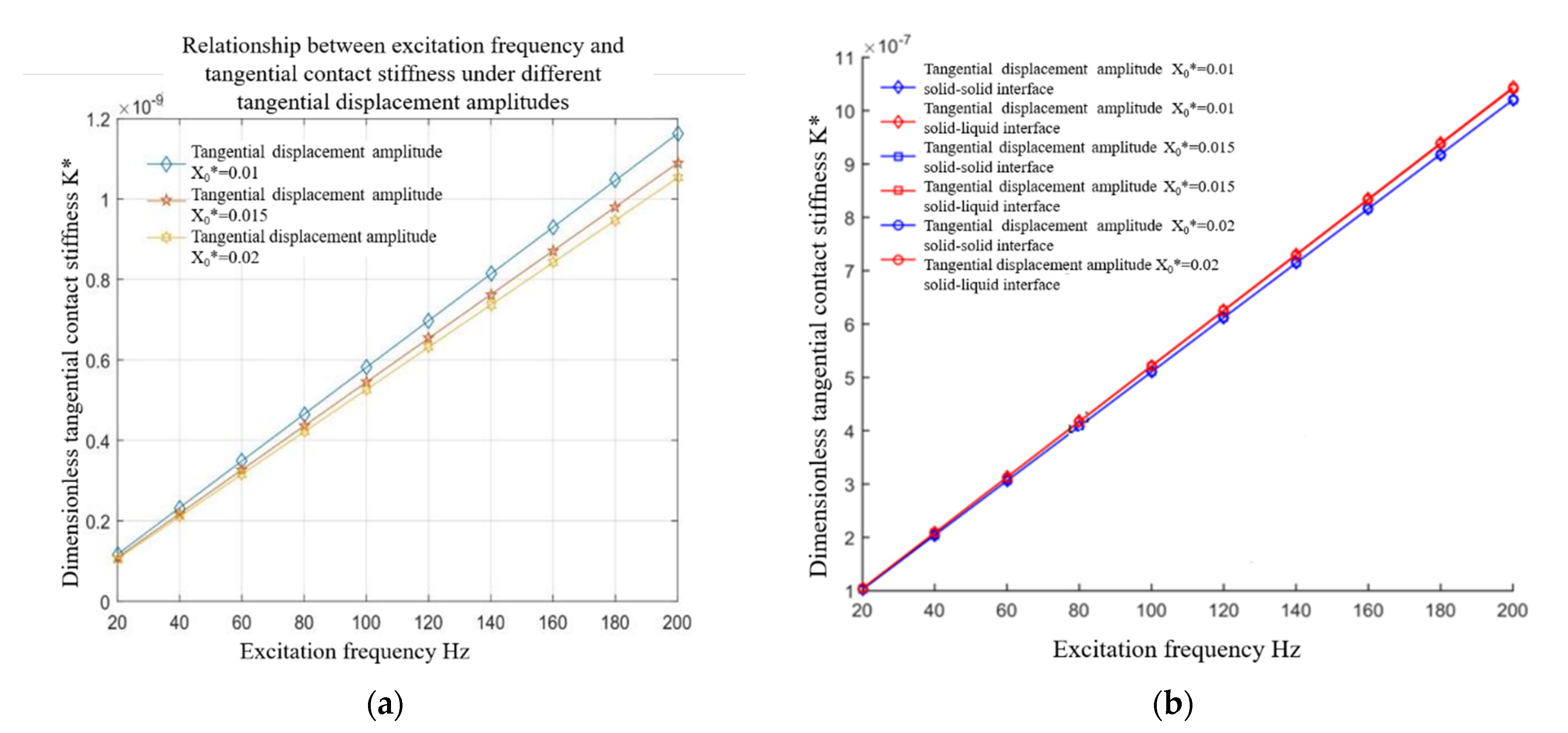
4.1.3. Effect of Excitation Frequency on Tangential Contact Stiffness

Figure 6a,b shows the variation of tangential contact stiffness of a fluid, solid–solid interface, and solid–liquid interface with an exciting frequency under a normal load of $2.664\times {10}^{-4}$ under different tangential displacement amplitudes. As can be seen from the diagram, the tangential contact stiffness of the three joints increases almost linearly with the increase in the excitation frequency, and different tangential displacement amplitudes have little effect on the tangential contact stiffness. This conclusion can be drawn from Equations (49)–(51) (solid part stiffness calculation formula) and Equations (15) and (22) (fluid part stiffness calculation formula). At the same frequency, the stiffness of the fluid part is one order of magnitude smaller than that of the solid part, so the solid–liquid interface shows the same trend as the solid–solid interface, and the numerical value is always slightly higher.

4.2. Simulation Analysis of Dynamic Tangential Damping of the Solid–Liquid Interface

4.2.1. Effect of a Normal Contact Load on Tangential Contact Damping

Figure 7a,b shows the variation of tangential contact damping of a fluid, solid–solid interface, and solid–liquid interface with a normal load at different excitation frequenciesunder the amplitude of dynamic relative displacement $X_0=15\times {10}^{-9}$ m. In Figure 7a, it is found that the tangential damping of the oil film increases almost linearly with the increase in the normal contact load. According toFigure 7b, it is found that the tangential damping of the solid–solid and solid–liquid interfaces increases nonlinearly with the increase in the normal contact load. From the microscopic point of view of the solid contact, with the increase in the normal contact load, the number of microconvex bodies in actual contact increases, the force needed to overcome friction in the tangential direction is greater, and the energy consumption increases, so tangential damping increases. From the point of view of a fluid, because the oil film’s shear force increases with the increase in the normal load, energy consumption increases accordingly, which leads to the increase in tangential damping, but under the same normal load, it is one order of magnitude smaller than the solid–solid interface, and the influence is small. Therefore, the variation trend of tangential damping of the solid–liquid interface with a normal contact load is consistent with that of the solid–solid interface and is always slightly higher than that of solid–solid interface.

4.2.2. Effect of Tangential Displacement Amplitude on Tangential Contact Damping

Figure 8a, b shows that the tangential contact damping coefficients of the solid–solid and solid–liquid interfaces vary with the amplitude of tangential dynamic displacement under a normal load of $2.664\times {10}^{-4}$ under different excitation frequencies. It can be seen from Figure 8b that the tangential damping coefficients of the solid–solid and solid–liquid interfaces under different excitation frequencies decrease nonlinearly with the increase in dynamic displacement amplitude. From the microscopic point of view of the solid contact, under a given normal load, the increase in the tangential displacement amplitude increases the number of micro-bumps in the micro-slip state, decreases the number of micro-bumps in the viscous state, and reduces friction energy consumption. As a result, the tangential contact damping of the bonding surface is reduced. It can be seen from Figure 8a that under the same conditions, the tangential contact damping of the oil film is almost constant, and the numerical value is one order of magnitude smaller than that of the solid–solid interface, so the variation trend of tangential contact damping of the solid−liquid interface with the amplitude of dynamic relative displacement is the same as that of the solid−solid interface, and the numerical value is always slightly higher.

4.2.3. Effect of Excitation Frequency on Tangential Damping

Figure 9a,b shows the variation of tangential damping of the solid–solid and solid–liquid interfaces with exciting frequency under a normal load of $2.664\times {10}^{-4}$ under different tangential displacement amplitudes.

It can be seen from Figure 9b that the tangential damping of the solid–solid and solid–liquid interfaces decreases nonlinearly with the increase in excitation frequency. From the microscopic point of view of the solid contact, under a given normal load, the increase in the excitation frequency makes the tangential displacement of the microconvex body unloaded before it has time to recover, and loaded again, resulting in the increase in the maximum tangential displacement and the decrease in energy dissipation. Therefore, the tangential contact damping is reduced. It can be seen from Figure 9a that under the same conditions, the tangential damping of the oil film decreases nonlinearly with the increase in excitation frequency, but it is an order of magnitude smaller than that of the solid–solid interface, so the change trend of the solid–liquid interface is the same as that of the solid–solid interface, and the value is always slightly higher.

5. Experimental Verification

In order to verify the correctness and validity of the tangential contact stiffness and damping model of the joint surface, the theoretical model was compared with the experimental results.

5.1. The Principle of the Experiment

When a solid–liquid surface is subjected to tangential static load and tangential excitation force, a macroscopic dynamics model is established for the solid–liquid surface, as shown in Figure 10.

In Figure 10, f is the tangential excitation force acting on the intermediate specimen; m₁ is the mass of the intermediate specimen; K_sum is the total tangential dynamic contact stiffness of the solid–liquid surface; C_sum is the total tangential dynamic damping coefficient of the solid–liquid surface; x₁ is the tangential relative displacement of the intermediate specimen; x₂ is the average tangential relative displacement of the left and right specimens.

Taking the intermediate specimen as the object of study, the following equation was used according to the solid–liquid bonding surface dynamics model:

$$m_1{\ddot{x}}_1+f_{\tau }=f$$

(56)

$$f_{\tau }=K_{sum}{x}_{\tau }+C_{sum}{\dot{x}}_{\tau }$$

(57)

where $x_{\tau }=x_1-x_2$,$\dot{ x_{\tau }}=\dot{x_1}-\dot{x_2}$.

For tangential simple harmonic excitation of the intermediate specimen, the effect of wave times at other frequencies can be disregarded.

$$f_{\tau }=F_{\tau }\cos wt$$

(58)

$$x_{\tau }=X_{\tau }\cos (\omega t+{\varphi }_{\tau })$$

(59)

$${\dot{x}}_{\tau }=X_{\tau }\omega \sin (\omega t+{\varphi }_{\tau })$$

(60)

Using Equations (58)–(60) in (57) provides us with the following:

$$K_{sum}=\frac{F_{\tau }\cos {\varphi }_{\tau }}{X_{\tau }}$$

(61)

$$C_{sum}=\frac{F_{\tau }\sin {\varphi }_{\tau }}{\omega X_{\tau }}$$

(62)

Let the area of the left and right test pieces be S. The expressions for the tangential dynamic contact stiffness and damping coefficient per unit area of the solid–liquid bond surface are as follows:

$$k_{\tau }=\frac{F_{\tau }\cos {\varphi }_{\tau }}{X_{\tau }S}$$

(63)

$$c_{\tau }=\frac{F_{\tau }\sin {\varphi }_{\tau }}{\omega X_{\tau }S}$$

(64)

where the units of $k_{\tau }$ and $c_{\tau }$ are $\mathrm{N}/\left(\mathsf{\mu }\mathrm{m}·{\mathrm{m}}^2\right)$ and $\mathrm{N}·\mathrm{s}/\left(\mathsf{\mu }\mathrm{m}·{\mathrm{m}}^2\right)$, respectively.

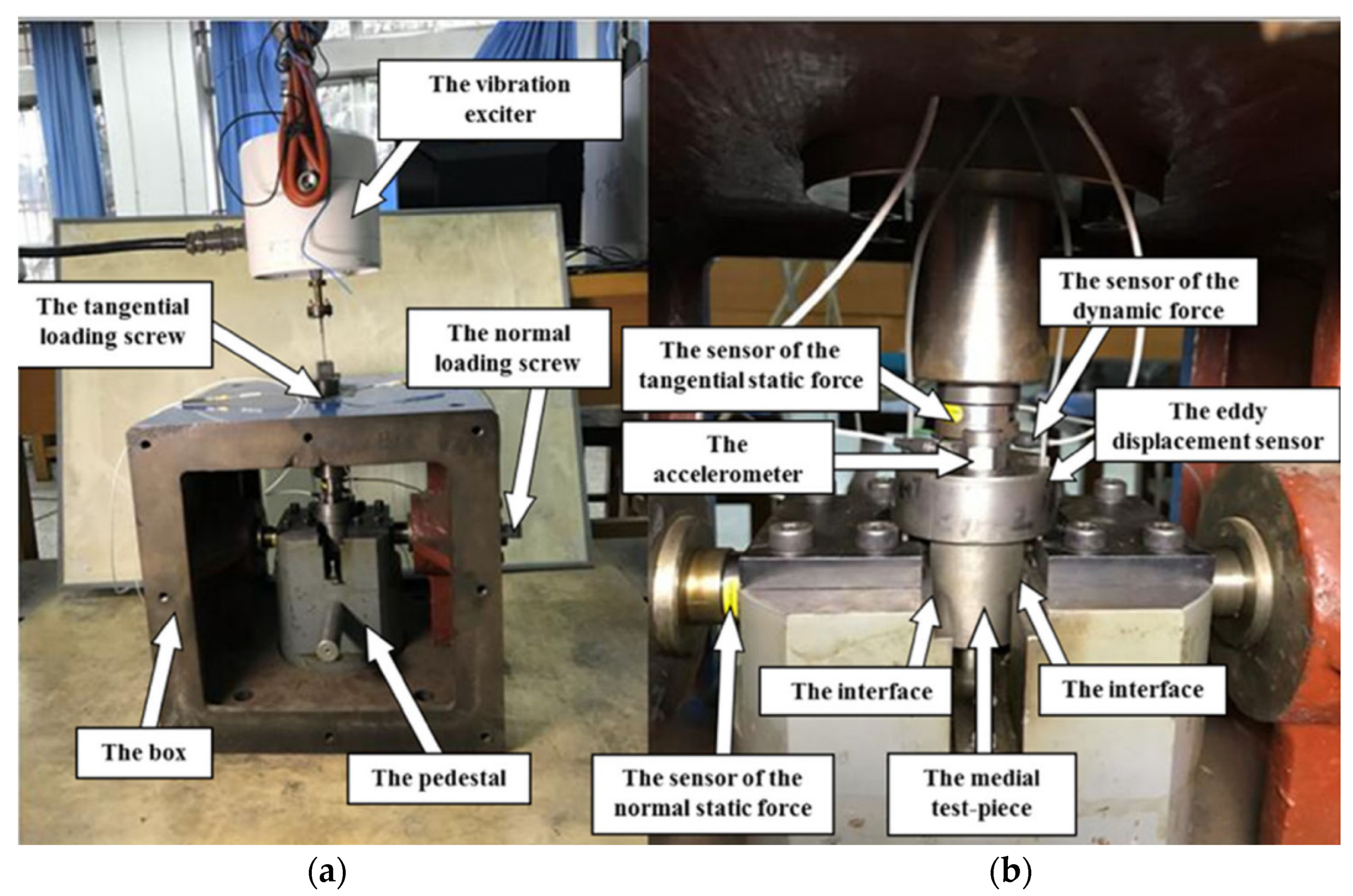
5.2. Experimental Device

This paper was based on the experimental platform built by Fu et al. [13,43], as shown in Figure 11a,b.

Figure 11a,b shows an experimental device of the tangential contact stiffness and damping and the layout of sensors. The interfaces were constructed by the middle test piece and the left–right test pieces. The force sensor was arranged at the middle test piece, which was used to test the static and dynamic force. All of the collected signals are analyzed by the m + p system, i.e., the m+p international SO Analyzer Rev. 4.0, where F_τ, X_τ, and ${\varphi }_{\tau }$ can be obtained by the m + p system. At first, f, ${\ddot{x}}_1$, and the phase difference ${\varphi }_{{\ddot{x}}_1}{}_{,f}$ between them, were measured by the force sensor and the accelerometers, respectively; x_τ and the phase difference ${\varphi }_{x_{\tau }}{}_{,f}$ between x_τ and f were directly measured by the pair of eddy–current displacement sensors fixed on the upper specimen. Next, force f_τ and phase difference ${\varphi }_{x_{\tau }}{}_{,f}$ between f_τ and f were obtained from Equation (56). At last, ${\varphi }_{x_{\tau }}{}_{,f}$ and ${\varphi }_{f_{\tau }}{}_{,f}$ lead to phase difference ${\varphi }_{\tau }$. The normal static preload, or normal pressure P_n, was measured by the force sensor.

In order to ensure the reliability of the experimental data, the experimental data need to be repeated several times before determining the average value. For example, the relationship between the tangential contact stiffness and damping and the tangential displacement amplitude is sought under the same face pressure and tangential excitation frequency. For this experiment, the damping stiffness at a certain displacement amplitude was obtained by first applying normal face pressure to the bonded surface to a fixed value, and then applying tangential excitation through the shaker to adjust it to 40Hz, and adjusting the displacement amplitude to 15nm to obtain the experimental data. After repeating this operation three times, three sets of experimental data were obtained, then the tangential stiffness and damping were calculated, and the average value of the three experiments was taken to obtain the final tangential stiffness and damping.

5.3. The Comparison between Theoretical Model and Experiment Results

The experiment using the same system conditions as the simulation, the upper/lower specimen test material is 45 steel, its material property parameter is $E_1=E_2=2.07\times {10}^{11}$ Pa, Poisson’s ratio ${\nu }_1={\nu }_2=0.29, H=1.96 \mathrm{G}$Pa, and the processing method is milling. Using the method of taking the surface parameters of the test specimen in reference [44], the micro-morphology statistical parameter of the contact surface is $\sigma /R=0.13$,$\beta =0.0029$, plasticity index $\psi =2.5$. It is assumed that the height of the microconvexbody is a Gaussian distribution. Kunlun Tianhong engine oil is selected as the lubricating medium of the solid–liquid interface. Its SAE viscosity is 5W-40, kinematic viscosity value at 40 °C is 82.4 mm²/s, kinematic viscosity value at 100 °C is 13.6 mm²/s, viscosity index is 170, and the density is 0.85 kg/m³. Under the above conditions, the experiments of stiffness and damping parameters of solid–liquid interface with and without lubricating medium were carried out respectively.

As shown in Figure 12a,b, the theoretical model and the experimental data show that the tangential contact stiffness and damping of the solid–solid and solid–liquid interfaces vary with normal load, in which the tangential excitation frequency is 40 Hz and the tangential displacement amplitude is 15 nm. From the experimental data in the diagram it can be found that the tangential contact stiffness and damping of the solid–liquid and solid–solid interfaces increase with the increase in contact load; under the same contact load, the contact stiffness and damping of the solid–liquid interface are larger than those of the solid–solid interface, and these trends are the same as the theoretical simulation results, which show that the simulation results are qualitatively consistent with the experimental results in magnitude and trend.

As shown in Figure 13a,b, the theoretical model and the experimental data show that the tangential contact stiffness and damping of the solid–solid and solid–liquid interfaces vary with excitation frequency, in which the normal load is 3.51 MPa and the tangential displacement amplitude is 15 nm. It can be seen from the experimental data that the tangential contact stiffness of the solid–solid and solid–liquid interfaces increases almost linearly with the increase in excitation frequency, and the tangential contact damping decreases nonlinearly with the increase in excitation frequency. The change trend of the theoretical model is basically consistent with the experimental data.

As shown in Figure 14a,b, the theoretical model and experimental data show that the tangential contact stiffness and damping coefficient of the solid–solid and solid–liquid interfaces vary with the amplitude of tangential displacement, where the normal load is 5.21 MPa and the tangential excitation frequency is 40 Hz. It can be seen from the experimental data that the tangential contact stiffness of the solid–solid and solid–liquid interfaces decreases nonlinearly with the increase of dynamic displacement amplitude, and the change trend is slow, and the tangential damping decreases nonlinearly with the increase in the dynamic displacement amplitude. The change trend is basically consistent with the theoretical results.

As can be seen in Figure 12, Figure 13 and Figure 14, the experimental results fo stiffness seem reasonable and match relatively well with theoretical results, damping results seem to be more scattered, with a less successful agreement with experiments. There are two possible reasons for the dispersion of the damping results and the less successful agreement with the experiments: (1) The theoretical model of damping was obtained from Equations (52) and (55), while the experimental data were obtained from Equation (64), and the principles were different, resulting in certain deviations; (2) from Equation (64), it is known that damping is influenced by the excitation frequency. During the experiment, the excitation signal was sent manually by the experimenter on the m+p dynamic analyzer, and the signal was transmitted to the shaker through the charge amplifier, and the shaker applied the excitation force to the intermediate specimen through the stinger. During the experiments, there were deviations between the set value of $\omega$ and the actual value applied to the device, as well as deviations in the value caused by external disturbances, which may result in a dispersion of the damping value of $\omega$. In contrast, the experimental value of stiffness was obtained using Equation (63), and its value was not affected by $\omega$. This may be the reason why the experimental data of stiffness were better than the experimental data of damping and the theoretical value.

6. Conclusions

In this paper, the modeling of tangential contact stiffness and damping of the solid–liquid interface under a tangential exciting force under mixed lubrication was studied. For the solid part, the loading/unloading stiffness and energy dissipation models of contact microconvex normal elastic/elastic–plastic/plastic deformation and tangential viscous and micro-slip states were established. The dynamic tangential contact stiffness and damping of the solid–solid interface were obtained using statistical theory and an equivalent viscous damping method. For the fluid part, the difference method was used to solve the average flow equation considering the roughness lubrication effect. According to the transient variation of the oil film’s shear force with displacement disturbance and velocity disturbance under tangential excitation, the dynamic tangential stiffness and damping of the oil film were obtained. Based on the stiffness and damping of the solid and fluid parts, the theoretical model of dynamic tangential contact stiffness and damping of the solid–liquid interface was established. The experimental results show that the theoretical model had the same change laws as the experimental results and is qualitatively consistent in magnitude and trend, which proves that the theoretical model is effective.

The results show that: (1) The tangential contact stiffness and damping of the solid–liquid and solid-solid interfaces belong to the same order of magnitude, and the value of the solid part is about one order of magnitude higher compared with that of the oil film part. It shows that the tangential contact stiffness and damping of the solid–liquid interface in the mixed-lubrication state are mainly determined by the solid–solid contact state under the action of a normal static preload and a tangential small vibration load, and the tangential contact stiffness and damping of the macroscopic static state are mainly determined by the solid–solid contact state. The influence of the oil film is small. (2) The normal contact load and the tangential exciting frequency have a great influence on the dynamic tangential contact stiffness, which increases almost linearly, that is, under the action of a larger normal contact load and a higher tangential exciting frequency, larger tangential contact stiffness of the solid–liquid interface can be obtained, but the influence of the dynamic tangential displacement amplitude is very small. (3) Normal contact load, tangential displacement amplitude, and exciting frequency have a significant influence on tangential contact damping. Increasing the normal contact load, decreasing the tangential displacement amplitude and the exciting frequency can help to increase the tangential contact damping.

References

1. Guozhong, D.; Hui, Z.; Yue, L.; Guangneng, D. Modeling and tribological characteristics of hybrid elastohydrodynamic lubrication system. J. Xi’an Jiaotong Univ. 2018, 52, 107–114. [Google Scholar]
2. Wang, X.; Zhao, X.; Xu, X.; Li, X.; He, K.; Tian, H. Mixed lubrication of a linear motion rolling guideway pair. J. Vib. Shock. 2020, 39, 260–266. [Google Scholar]
3. Carrella, A.; Brennan, M.J.; Waters, T.P.; Lopes, V., Jr. Force and displacement transmissibility of a nonlinear isolator with high-static-low-dynamic-stiffness. Int. J. Mech. Sci. 2012, 55, 22–29. [Google Scholar] [CrossRef]
4. Zou, H.; Wang, B. Investigation of the contact stiffness variation of linear rolling guides due to the effects of friction and wear during operation. Tribol. Int. 2015, 92, 472–484. [Google Scholar] [CrossRef]
5. Li, X.P.; Pan, W.J.; Gao, J.Z.; Li, S.J.; Zhao, G.H.; Wen, B.C. Influence of surface topography characteristics on mode coupling instability system. J. Mech. Eng. 2017, 53, 116–127. [Google Scholar] [CrossRef]
6. Oh, K.-J.; Cao, L.; Chung, S.-C. Explicit modeling and investigation of friction torques in double-nut ball screws for the precision design of ball screw feed drives. Tribol. Int. 2020, 141, 105841. [Google Scholar] [CrossRef]
7. Zheng, F.Y. Theory and application of variable speed gear transmission with moving shaft. J. Mech. Eng. 2019, 55, 52–64. [Google Scholar]
8. Liu, J.; Ma, C.; Wang, S. Precision loss modeling method of ball screw pair. Mechanical Syst. Signal Process. 2020, 135, 106397. [Google Scholar] [CrossRef]
9. Gonzalez-Valadez, M.; Dwyer-Joyce, R.; Lewis, R. Ultrasonic reflection from mixed liquid-solid contacts and the determination of interface stiffness. In Tribology and Interface Engineering Series; Elsevier: Amsterdam, The Netherlands, 2005; Volume 48, pp. 313–320. [Google Scholar]
10. Dwyer-Joyce, R.; Reddyhoff, T.; Zhu, J. Ultrasonic measurement for film thickness and solid contact in elastohydrodynamic lubrication. J. Tribol. 2011, 133, 407–411. [Google Scholar] [CrossRef]
11. Shi, X.; Polycarpou, A.A. Measurement and modeling of normal contact stiffness and contact damping at the meso scale. J. Vib. Acoust. 2005, 127, 52–60. [Google Scholar] [CrossRef]
12. Ren, P.; Wang, L.H.; Wang, C.F. Experimental study on normal dynamic contact stiffness of guide joint under lubrication. China Mech. Eng. 2018, 29, 811–816. [Google Scholar]
13. Fu, W.P.; Lou, L.T.; Gao, Z.Q.; Wang, W.; Wu, J.B. Theoretical model of normal contact stiffness and damping of mechanical joint. J. Mech. Eng. 2017, 53, 73–82. [Google Scholar] [CrossRef]
14. Ma, C.; Duan, Y.; Yu, B.; Sun, J.; Tu, Q. The comprehensive effect of surface texture and roughness under hydrodynamic and mixed lubrication conditions. Proc. Inst. Mech. Eng. Part J. J. Eng. Tribol. 2017, 231, 1307–1319. [Google Scholar] [CrossRef]
15. Xiao, H.F.; Sun, Y.Y.; Xu, J.W. Study on calculation model and characteristics of normal contact stiffness of rough interface under mixed lubrication. Vib. Shock. 2018, 37, 106–114+147. [Google Scholar]
16. Sun, Y.; Xiao, H.; Xu, J.; Yu, W. Study on the normal contact stiffness of the fractal rough surface in mixed lubrication. Proc. Inst. Mech. Eng. Part. J. J. Eng. Tribol. 2018, 232, 1604–1617. [Google Scholar] [CrossRef]
17. Li, L.; Yun, Q.Q.; Li, Z.Q.; Cai, A.J.; Duan, Z.S. Contact characteristics of joint surfaces considering bulk substrate deformation in mixed lubrication. Vib. Test Diagn. 2019, 39, 953–959+1128–1129. [Google Scholar]
18. Li, L.; Pei, X.Y.; Shi, X.H.; Li, Z.Q.; Cai, A.J. Study on normal contact stiffness of joint under mixed lubrication. Vib. Shock. 2020, 39, 16–23. [Google Scholar]
19. Wen, X.Y.; Zhang, X.L.; Tan, W.B.; Zhang, W. Study on three-dimensional Fractal Model of normal contact stiffness of mixed Lubrication Joint Surface. Modul. Mach. Tool Autom. Mach. Technol. 2020, 11, 49–53. [Google Scholar]
20. Zhou, C.J.; Xiao, Z.L.; Chen, S.Y.; Han, X. Normal and tangential oil film stiffness of modified spur gear with non-Newtonian elastohydrodynamic lubrication. Tribiology Int. 2016, 109, 319–327. [Google Scholar] [CrossRef]
21. Zhou, C.J.; Xiao, Z.L. Stiffness and damping models for the oil film in line contact elastohydrodynamic lubrication and applications in the gear drive. Appl. Math. Model. 2018, 61, 634–649. [Google Scholar] [CrossRef]
22. Jones, R.E. A Greenwood-Williamson model of small-scale friction. J. Appl. Mech. 2007, 74, 31–40. [Google Scholar] [CrossRef]
23. Wang, J.; Chen, T.; Wang, X.; Xi, Y. Dynamic identification of tangential contact stiffness by using friction damping in moving contact. Tribol. Int. 2019, 131, 308–317. [Google Scholar] [CrossRef]
24. Wu, J.; Yuan, R.; He, Z.; Zhang, D.; Xie, Y. Experimental study on dry friction damping characteristics of the steam turbine blade material with nonconforming contacts. Adv. Mater. Sci. Eng. 2015, 2015, 849253. [Google Scholar] [CrossRef]
25. Eriten, M.; Chen, S.; Usta, A.D.; Yerrapragada, K. In Situ Investigation of Load-Dependent Nonlinearities in Tangential Stiffness and Damping of Spherical Contacts. J. Tribol. 2021, 143, 061501. [Google Scholar] [CrossRef]
26. Wen, S.Z.; Huang, P. Principles of Tribology, 2nd ed.; Qinghua University Press: Beijing, China, 2002. [Google Scholar]
27. Schlichting, H.; Kestin, J. Boundary Layer Theory; Springer: Berlin/Heidelberg, Germany, 2017. [Google Scholar]
28. Wu, C.; Zheng, L. An average Reynolds equation for partial film lubrication with a contact factor. J. Tribol. 1989, 111, 188–191. [Google Scholar] [CrossRef]
29. Li, R.H. Numerical Solution of Partial Differential Equation; Higher Education Press: Beijing, China, 2005. [Google Scholar]
30. Ma, C.B. Study on Lubrication Calculation Model and Antifriction Characteristics of Textured Surface. Ph.D. Thesis, China University of Mining and Technology, Beijing, China, 2010. [Google Scholar]
31. Rowe, W.; Chong, F. Computation of dynamic force coefficients for hybrid (hydrostatic/hydrodynamic) journal bearings by the finite disturbance and perturbation techniques. Tribol. Int. 1986, 19, 260–271. [Google Scholar] [CrossRef]
32. Ma, C.B. Study on Lubrication calculation Model and antifriction characteristics of textured Surface. J. Mech. Eng. 2007, 3, 95–101. [Google Scholar]
33. Kadin, Y.; Kligerman, Y.; Etsion, I. Unloading an elastic–plastic contact of rough surfaces. J. Mech. Phys. Solids 2006, 54, 2652–2674. [Google Scholar] [CrossRef]
34. Fujimoto, T.; Kagami, J.; Kawaguchi, T.; Hatazawa, T. Micro-displacement characteristics under tangential force. Wear 2000, 241, 136–142. [Google Scholar] [CrossRef]
35. Gao, Z.Q. Study on the Theoretical Model of Contact Stiffness and Damping of Mechanical Joint. Ph.D. Thesis, Xi’an University of Technology, Xi’an, China, 2018. [Google Scholar]
36. Kogut, L.; Etsion, I. Elastic-plastic contact analysis of a sphere and a rigid flat. J. Appl. Mech. 2002, 69, 657–662. [Google Scholar] [CrossRef]
37. Gorbatikh, L.; Popova, M. Modeling of a locking mechanism between two rough surfaces under cyclic loading. Int. J. Mech. Sci. 2006, 48, 1014–1020. [Google Scholar] [CrossRef]
38. Thornton, C.; Ning, Z. A theoretical model for the stick/bounce behaviour of adhesive, elastic-plastic spheres. Powder Technol. 1998, 99, 154–162. [Google Scholar] [CrossRef]
39. Thornton, C.; Ning, Z.; Chuan-yu, W.; Nasrullah, M.; Long-yuan, L. Contact mechanics and coefficients of restitution. In Granular Gases; Springer: Berlin/Heidelberg, Germany, 2001; pp. 184–194. [Google Scholar]
40. Thornton, C. Coefficient of restitution for collinear collisions of elastic-perfectly plastic spheres. J. Appl. Mech. 1997, 64, 383–386. [Google Scholar] [CrossRef]
41. He, S.M.; Wu, Y.; Shen, J. Microscopic displacement characteristics of elastic-plastic materials under tangential load. Eng. Mech. 2010, 27, 73–77. [Google Scholar]
42. Dai, D.P. Damping Vibration and Noise Reduction Technology; Xi’an Jiaotong University: Xi’an, China, 1986. [Google Scholar]
43. Fu, W.P.; Gao, Z.Q.; Wang, W.; Wu, J.B. A Model of Tangential Contact Damping Considering Asperity Interaction and Lateral Contact. Acta Mech Solida Sin. 2018, 31, 758–774. [Google Scholar] [CrossRef]
44. Liang, J.W.; Feeny, B.F. Identifying Coulomb and Viscous Friction from Free-Vibration Decrements. Nonlin Dyn. 1998, 16, 337–347. [Google Scholar] [CrossRef]
Figure 1. Calculation process of tangential stiffness and damping of the fluid part of the solid–liquid interface.
Machines 10 00804 g001
Figure 2. Rough surface and rigid smooth surface.
Machines 10 00804 g002
Figure 3. Stick–slip contact model of the microconvex body.
Machines 10 00804 g003
Figure 4. Relationship between the tangential contact stiffness of a solid−solid interface and a solid–liquid interface and a normal contact load. (a) Fluid contact characteristics, (b) solid−solid to solid−liquid interfaces.
Machines 10 00804 g004
Figure 5. Relationship between the tangential contact stiffness and the tangential displacement amplitude under different excitation frequencies. (a) Fluid contact characteristics, (b) solid−solid and solid−liquid bonding face ratio.
Machines 10 00804 g005
Figure 6. Relationship between the tangential contact stiffness and the excitation frequency under different tangential displacement amplitudes. (a) Fluid contact characteristics, (b) solid−solid and solid−liquid bonding face ratio.
Machines 10 00804 g006
Figure 7. Relationship between the tangential damping coefficient and a normal contact load under different excitation frequencies. (a) Fluid contact characteristics, (b) solid−solid and solid–liquid bonding face ratio.
Machines 10 00804 g007
Figure 8. Relationship between the tangential displacement amplitude and the tangential damping coefficient of the solid–solid and solid–liquid interfaces under different excitation frequencies. (a) Fluid contact characteristics, (b) solid–solid and solid–liquid bonding face ratio.
Machines 10 00804 g008
Figure 9. Relationship between the excitation frequency and the tangential damping coefficient of the solid–solid and solid–liquid interfaces under different tangential displacement amplitudes. (a) Fluid contact characteristics, (b) solid–solid and solid–liquid bonding face ratio.
Machines 10 00804 g009
Figure 10. Tangential mechanical model of the solid–liquid interface.
Machines 10 00804 g010
Figure 11. Experimental device of the tangential contact stiffness and damping.(a) Experimental box. (b) The layout of sensors.
Machines 10 00804 g011
Figure 12. Comparative verification of the theoretical model and the experimental data of tangential contact stiffness and damping varying with normal load. (a) Tangential contact stiffness, (b) tangential contact damping.
Machines 10 00804 g012
Figure 13. Comparison and verification of the theoretical model and the experimental data of dynamic characteristic parameters varying with frequency. (a) Tangential contact stiffness, (b) tangential contact damping.
Machines 10 00804 g013
Figure 14. Comparative verification of the theoretical model and the experimental data of tangential contact stiffness and damping varying with displacement amplitude. (a) Tangential contact stiffness, (b) tangential contact damping.
Machines 10 00804 g014
Publisher’s Note: MDPI stays neutral with regard to jurisdictional claims in published maps and institutional affiliations.