Article

Singularity Analysis and Geometric Optimization of a 6-DOF Parallel Robot for SILS

1
Research Center for Industrial Robots Simulation and Testing CESTER, Technical University of Cluj-Napoca, 400641 Cluj-Napoca, Romania
2
Department of Urology, Iuliu Hatieganu University of Medicine and Pharmacy, 400000 Cluj-Napoca, Romania
3
Department of Internal Medicine, Iuliu Hatieganu University of Medicine and Pharmacy, 400000 Cluj-Napoca, Romania
*
Author to whom correspondence should be addressed.
Machines 2022, 10(9), 764; https://doi.org/10.3390/machines10090764
Submission received: 29 July 2022 / Revised: 25 August 2022 / Accepted: 29 August 2022 / Published: 2 September 2022
(This article belongs to the Special Issue New Frontiers in Parallel Robots)

Abstract

:
The paper presents the singularity analysis and the geometric optimization of a 6-DOF (Degrees of Freedom) parallel robot for SILS (Single-Incision Laparoscopic Surgery). Based on a defined set of input/output constraint equations, the singularities of the parallel robotic system are determined and geometrically interpreted. Then, the geometric parameters (e.g., the lengths of the mechanism links) for the 6-DOF parallel robot for SILS are optimized such that the robotic system complies with an operational workspace defined in correlation with the SILS task. A numerical analysis of the singularities showed that the operational workspace is singularity free. Furthermore, numerical simulations validate the parallel robot for the next developing stages (e.g., designing and prototyping stages).

1. Introduction

Single-incision laparoscopic surgery (SILS) is a type of minimally invasive surgery (MIS) where the surgeon uses a special multi-lumen trocar (a trocar with multiple insertion points) inserted through a single incision in the patient body for all instruments required for surgery. SILS was described in the gynecological literature as early as 1969, when Wheesess reported the first 4.000 cases of tubal ligation [1]. As the literature suggests, the main advantages of SILS are: (i) the short recovery time for the patient, (ii) lesser degree of pain (when compared to classical MIS), (iii) and better cosmetics (since it uses a single access port) [2]. However, the challenges of SILS (performed manually) are caused by its poor ergonomics [3]. As history shows, robotic systems for surgery were developed to circumvent various limitations of the classical, human-performed interventions. MIS is one example in which robots had a significant impact [4,5]. Multiple approaches have been proposed and developed for robotic systems for MIS, namely: multi-arm robotic systems [4], flexible robotic systems [4], laparoscope holders [6], etc. The analysis of the intraoperative data from robotic surgery has enabled the addition of new technologies, one of them referring to automated gesture recognition, which assists the surgeon during delicate procedures such as suturing. For this task, multiple intelligent algorithms were developed using supervised, unsupervised, or semi-supervised learning paradigms [7]. This is an important step toward autonomous robotic-assisted surgery, where the robot uses a confidence-based shared control strategy to perform certain tasks under supervision but without the involvement of the human operator [8]. The advancements in computer science, which are now providing more reliable intelligent algorithms and the increased availability of large quantities of information (big data)—pre-operative digital information, instruments motion for repetitive tasks, recorded surgeries, patient evolution in the short and long term—are indicators and supporters of the next generation of devices, intelligent surgical robots [9].
The year 2018 marks the starting point for surgical robots dedicated to SILS due to the first use of the robotic da Vinci SP system in SILS surgery [4,10,11]. The da Vinci SP robot received FDA approval in 2018, becoming a benchmark in SILS robotic surgery, with a serial architecture capable of manipulating and orienting active instruments and the laparoscopic camera by using a single port through which these instruments are inserted. The system has an articulated laparoscopic camera and instruments, thus offering much better visibility and dexterity in the operating field compared to classical instruments [12]. The drawbacks are the limited forces (for tissue manipulation) due to the multiple bends of the instruments. Another robot dedicated to SILS surgery that has received FDA approval is the Senhance robot, which in contrast to da Vinci SP is a multi-arm system with three independent serial manipulators capable of orienting and manipulating surgical instruments [13]. Furthermore, there are various robotic systems for SILS which have not yet received FDA approval, such as SORT, SPIDER, MASTER, Virtual Incision, and so on [4].
Since a robotic system for SILS must comply with complex design specifications (e.g., footprint in the operating room, occupied volume, quick removal in case of an emergency), various optimizations are achieved in the early design stages. In a general interpretation, optimization aims to find the best solution for a given problem based on the imposed restrictions. In robotics, the optimization process often faces conflicting criteria such as speed versus energy efficiency, accuracy versus stability, or geometric dimensions versus working volume. When dealing with multi-objective optimization problems, the results are often given as a set of Pareto optimal solutions which must be further interpreted. In [14], the authors present an optimal dimensional synthesis of a parallel mechanism using two objective functions: finding the smallest dimensions for the geometric links of the robot for a given workspace, and the second aims to ensure the best overall dexterity within this workspace. As the two functions have conflicting criteria, it was shown that favoring the first function can lead to a robot with low dexterity while the second leads to a bulky robot. A numerical optimization methodology is presented in [15] to achieve an optimal design synthesis for a planar parallel manipulator for a prescribed dexterous workspace, using the condition number (an index that describes the dexterity of a robot). Merlet emphasizes in [16] the importance of the proper use of the condition number and global conditioning index (GCI) in the optimal design of a robot, illustrating their limitations (namely, when they are applied to robots that have both translation and orientation motions). GCI was first introduced by Gosselin and Angeles in [17], and it was one of the first approaches to describe the global performance of a manipulator, also demonstrating that in some cases, GCI can provide conflicting results in workspace optimization problems. In [18], the authors successfully applied the GCI and condition number to a 2-DOF parallel mechanism enabling them to obtain a generalized characterization of the manipulator with respect to its operational workspace. In [19], the authors used the condition number to optimize Orthoglide, a 3-DOF parallel robot with only translational motions used in milling applications. The dimensional synthesis of the 3-DOF Delta parallel robot for a prescribed workspace is presented in [20], where the authors define several optimization objectives solved using the Lagrange multipliers method, demonstrating that existing industrial robots could have almost half their size for the same given workspace. Furthermore, for a Delta-like parallel robot, in [21], the authors achieved an optimum design using multi-objective optimization algorithms, i.e., Pareto-optimization. A methodology to achieve an optimal design for a 6-DOF parallel manipulator having as objective its accuracy is presented in [22], where the authors are using the distribution of the condition number to determine the best solutions. The Stewart–Gough platform was analyzed in detail in [23], where the authors used a multi-objective optimization algorithm (NSGA-II) to obtain the optimal geometric parameters and leg stroke lengths, demonstrating that this approach is more efficient than the classical numerical methods. The workspace maximization of the Delta robot using a geometrical technique implemented in CATIA is shown in [24], where the use of the Simulated Annealing Algorithm provided promising results. The process of optimization is also found in the scientific literature concerning the development of medical robots. In [25], the authors optimized a 3-DOF serial robot considering the robot workspace and the surgical instrument insertion points. Other authors [26] used optimization processes for the static balancing of a surgical robot.
A novel approach for robotic-assisted SILS was proposed in [27], which is based on hybrid robotic systems with three major components: (1) a 6-DOF parallel robot that simultaneously guides (2) two interconnected orientation platforms (mounted on the mobile platform of the 6-DOF parallel robot) together with a laparoscopic camera, and (3) two active surgical instruments (mounted in the orientation platforms) to perform the SILS task. The kinematics of the surgical instruments was studied in [28], and in [29], the input–output equations for the orientation platform were provided. Furthermore, a recent work [27] achieved the kinematic modelling of the 6-DOF parallel robot.
The present paper illustrates the results regarding the further development of the SILS robotic system, namely: (i) a singularity analysis for the 6-DOF parallel robot presented in [27] (correlated with the operational workspace of the robot) and (ii) a geometric optimization of the 6-DOF parallel robot, to reduce its operating room footprint while maintaining the capabilities of performing the SILS task in a defined operational workspace. The singularity analysis was achieved using the vanishing conditions of the Jacobian matrices A and B. The input singularities are straightforward to interpret for the 6-DOF parallel robot, and for the output singularities, a geometric interpretation was achieved based on the characteristic tetrahedron [30]. For the geometric optimization, the Multi-Objective Genetic Algorithm implemented in Matlab gamultiobj function [31] is used to minimize the dimensions of the robot for a defined operational workspace. The GCI index is used in the optimization process only as guidance and not as a decision parameter due to its drawbacks when used on robots that have both translation and orientation motions [16,17].
The paper is structured as follows: Section 2 defines the parallel robotic system with all its modules and presents the inverse geometric model for the 6-DOF parallel robot. Section 3 defines the robotic system’s operational workspace to create a clear description of the robotic system task. Section 4 presents a singularity analysis for the general 6-DOF parallel robot. Section 5 presents the proposed optimization algorithm for the 6-DOF parallel robot and the general optimization criteria. Section 6 presents the optimized version of the 6-DOF parallel robot, showing that the operational workspace is singularity free. Furthermore, numerical simulations are provided to validate the optimized robotic system. The conclusions are presented in Section 7.

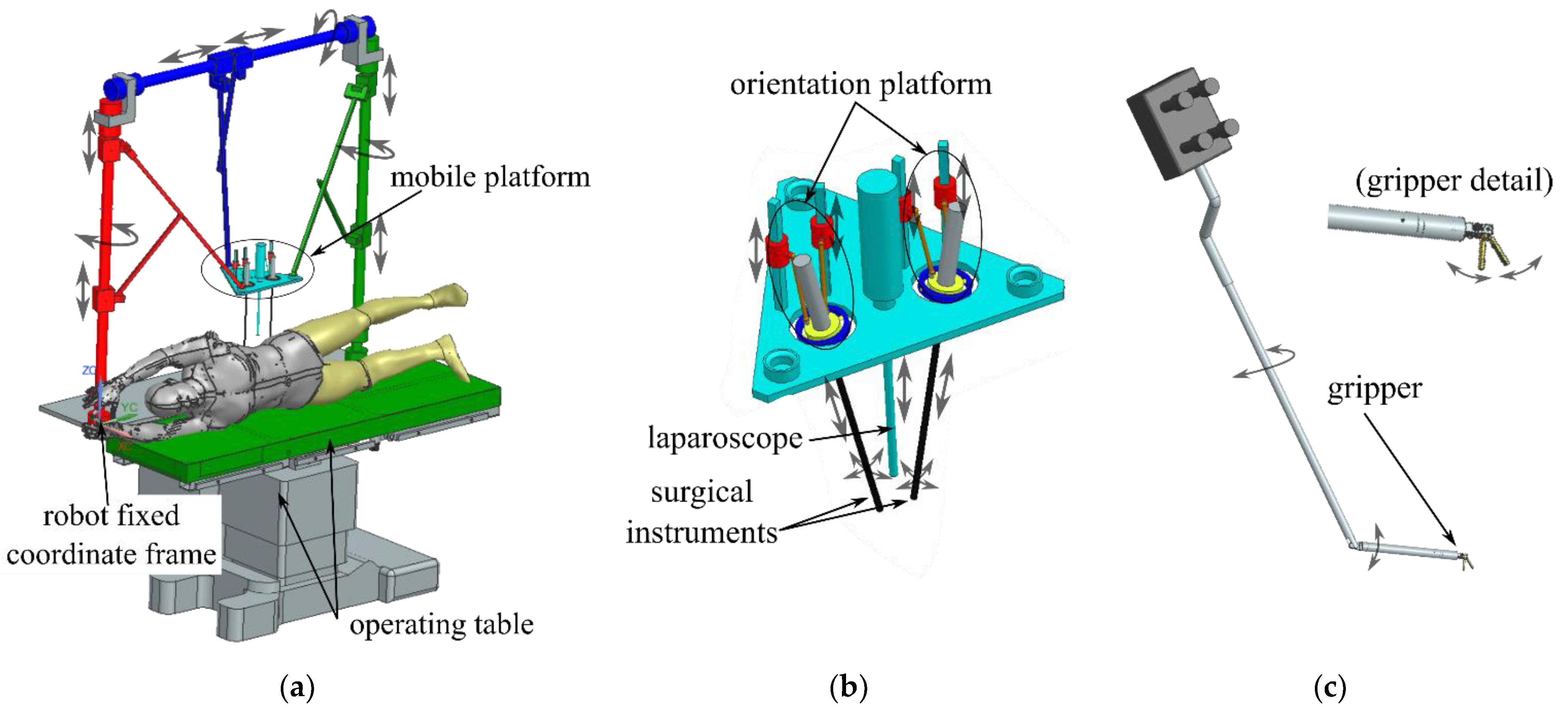
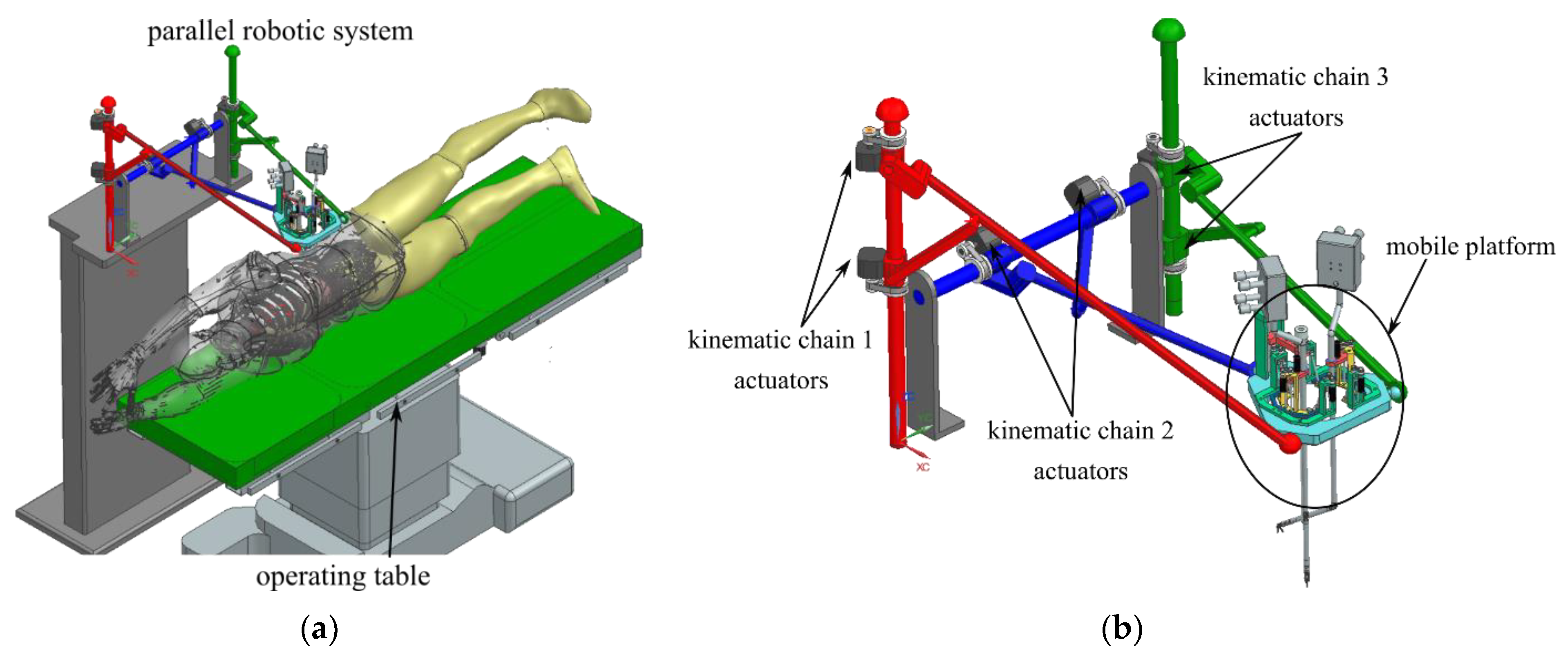
2. An Innovative Parallel Robotic System for SILS

SILS requires the simultaneous independent manipulation of two surgical instruments while the operating field is viewed through a laparoscopic camera. The position of the laparoscope is not fixed, and it can change depending on the target tissue location. Furthermore, both the surgical instruments and the laparoscope must be manipulated with respect to Remote Center of Motion (RCM) points, i.e., the insertion points of the instrument within the trocar. Lastly, the position of the insertion points (or the trocar) on the patient’s abdomen may vary based on various medical factors (e.g., the position of the resected tissue, areas that must be avoided, etc.) [3].
To comply with the required design parameters, an innovative parallel robotic system for SILS was proposed with the following components:
  • One 6-DOF parallel robot (patent pending [32])—guides a triangular mobile platform (Figure 1a) that contains a 1-DOF insertion mechanism for the laparoscopic camera;
  • Two 3-DOF orientation platforms (described in [29])—both mounted on the mobile platform (Figure 1b) on the sides of the laparoscopic camera insertion mechanism. The orientation platform can orient the surgical instruments using RCM with 2-DOF. The third DOF is for the linear insertion/retraction of the surgical instrument;
  • Two surgical instruments (described in [28])—each mounted in one orientation platform. Each surgical instrument has a serial architecture with 4-DOF: 1-DOF for the rotation about its longitudinal axis (the third rotation for the surgical instrument), 1-DOF for the (articulated) bending, and 2-DOF for the gripper (each jaw of the gripper is actuated separately enabling grabbing and gripper turning) (Figure 1c).
With respect to a defined robotic-assisted medical protocol [3], the proposed robotic system must comply with the following stepwise procedure:
  • A preplanning procedure is performed to establish the adequate therapeutic conduit, also with respect to the robotic-assisted medical task. Among other medical parameters (patient history, etc.), the patient position is established, insertion points for the instruments are defined, and the relative position of the robot with respect to the insertion points is defined to ensure the required ranges of motions for the surgical instruments;
  • The 6-DOF parallel robot positions the mobile platform at the trocar (insertion points) and inserts the laparoscope and the surgical instruments on a linear trajectory. Due to the mechanically constrained RCM position (near the mobile platform), the 6-DOF parallel robot guides the mobile platform in close proximity to the patient;
  • The combined motion of the 3-DOF orientation platforms and the 4-DOF surgical instruments allows the surgeon to perform the task from the control console;
  • The laparoscope position can be adjusted by reorienting the mobile platform. Consequently, the laparoscope RCM must be maintained through the robot control, and simultaneously, the instrument position must be corrected by the 3-DOF orientation platforms (e.g., to maintain the instrument gripper-tissue relative position while changing the laparoscope position).
The kinematic scheme of the 6-DOF parallel robot is presented in Figure 2. Although the mechanism topology is the same as in [27], in this work, the kinematic chains are not considered identical (removing this design constraint may improve the final solution for the robot architecture). In [27], the links l2, l3, and l4 had the same values.
The 6-DOF parallel robot mechanism topology is as follows [27]:
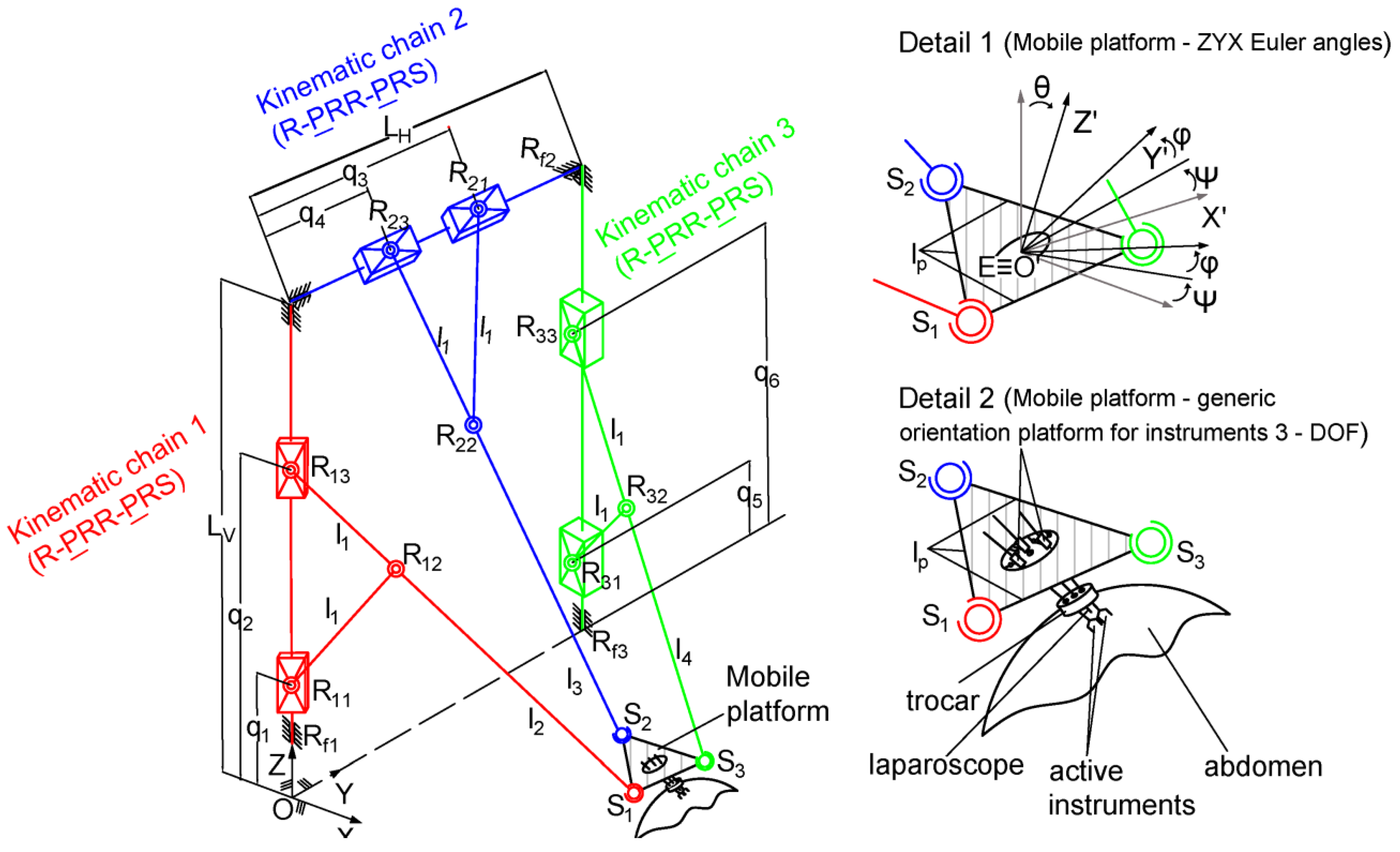
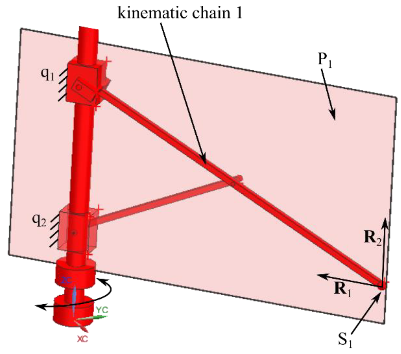
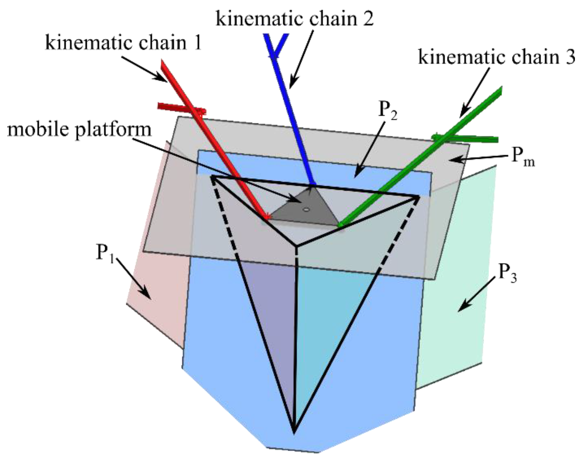
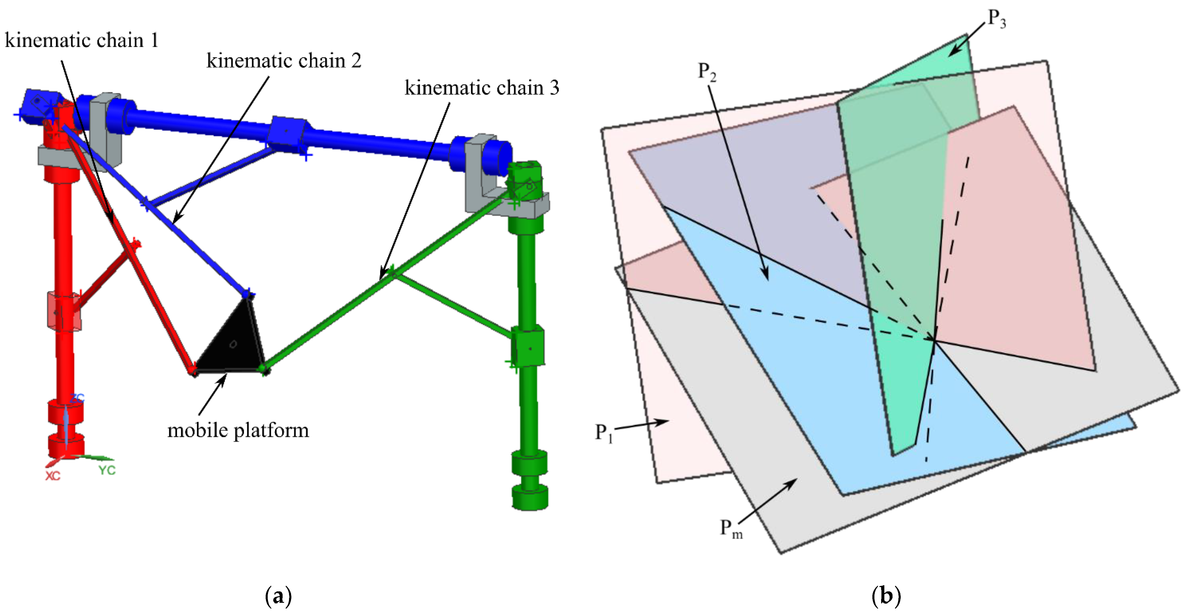
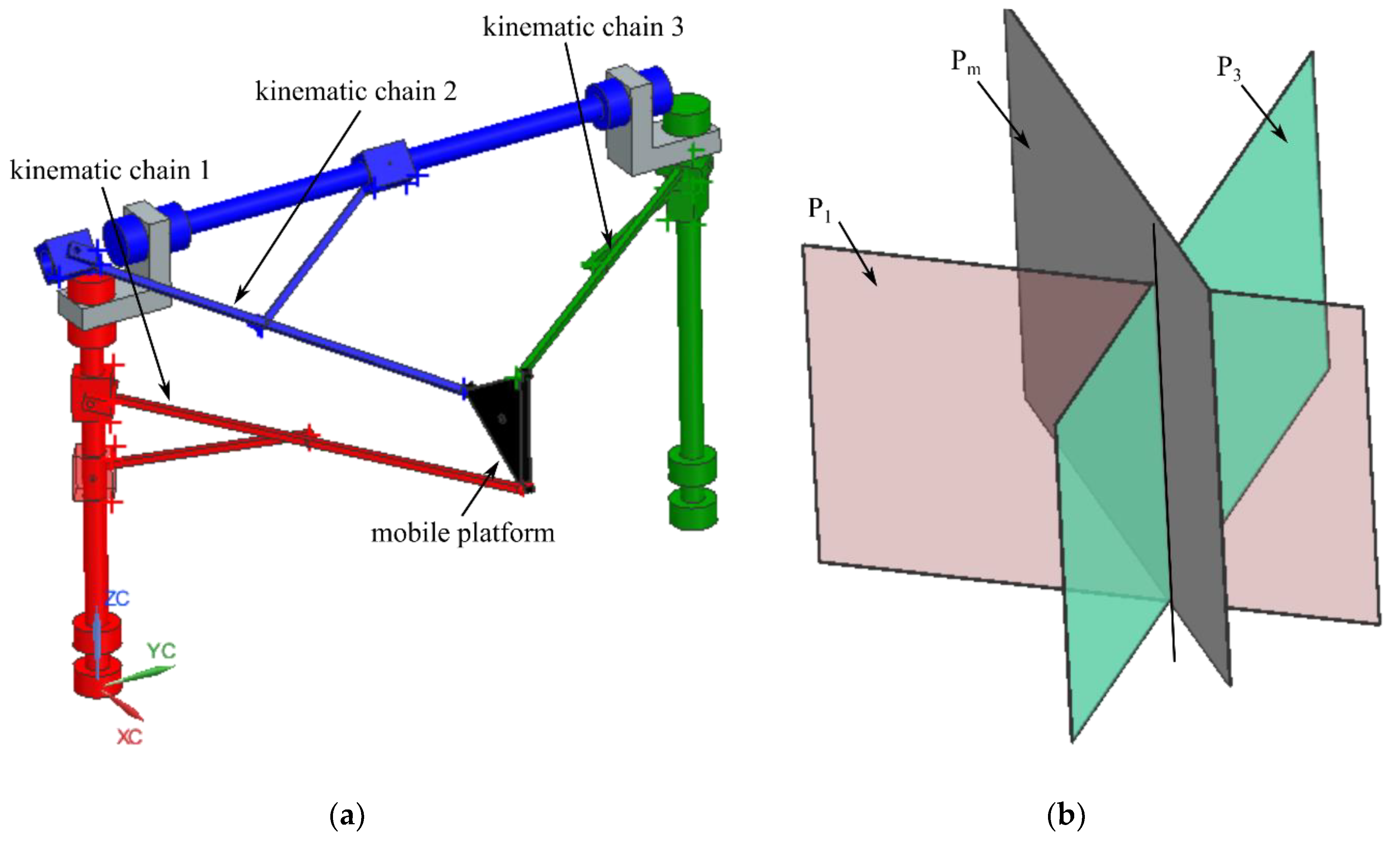
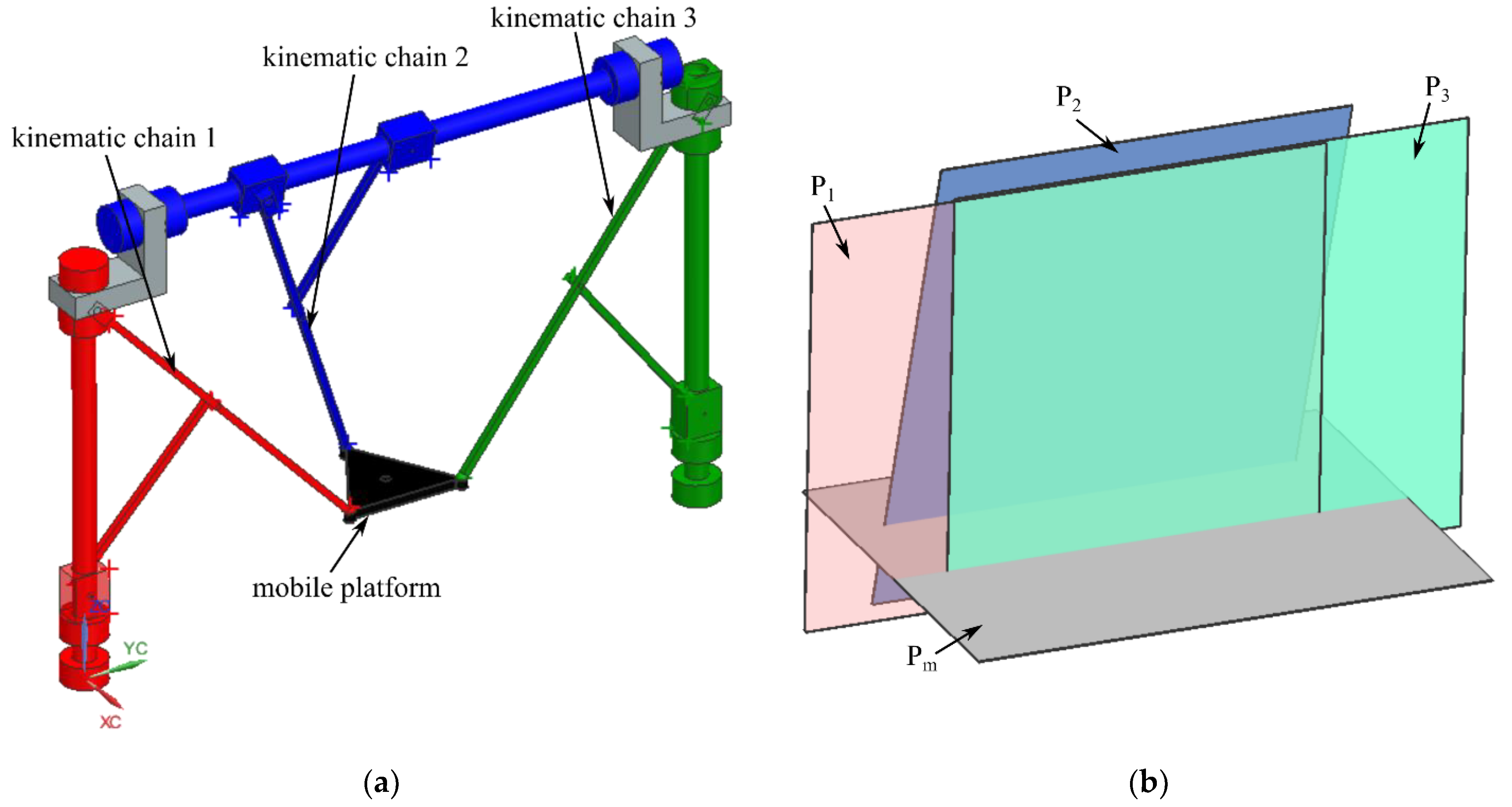
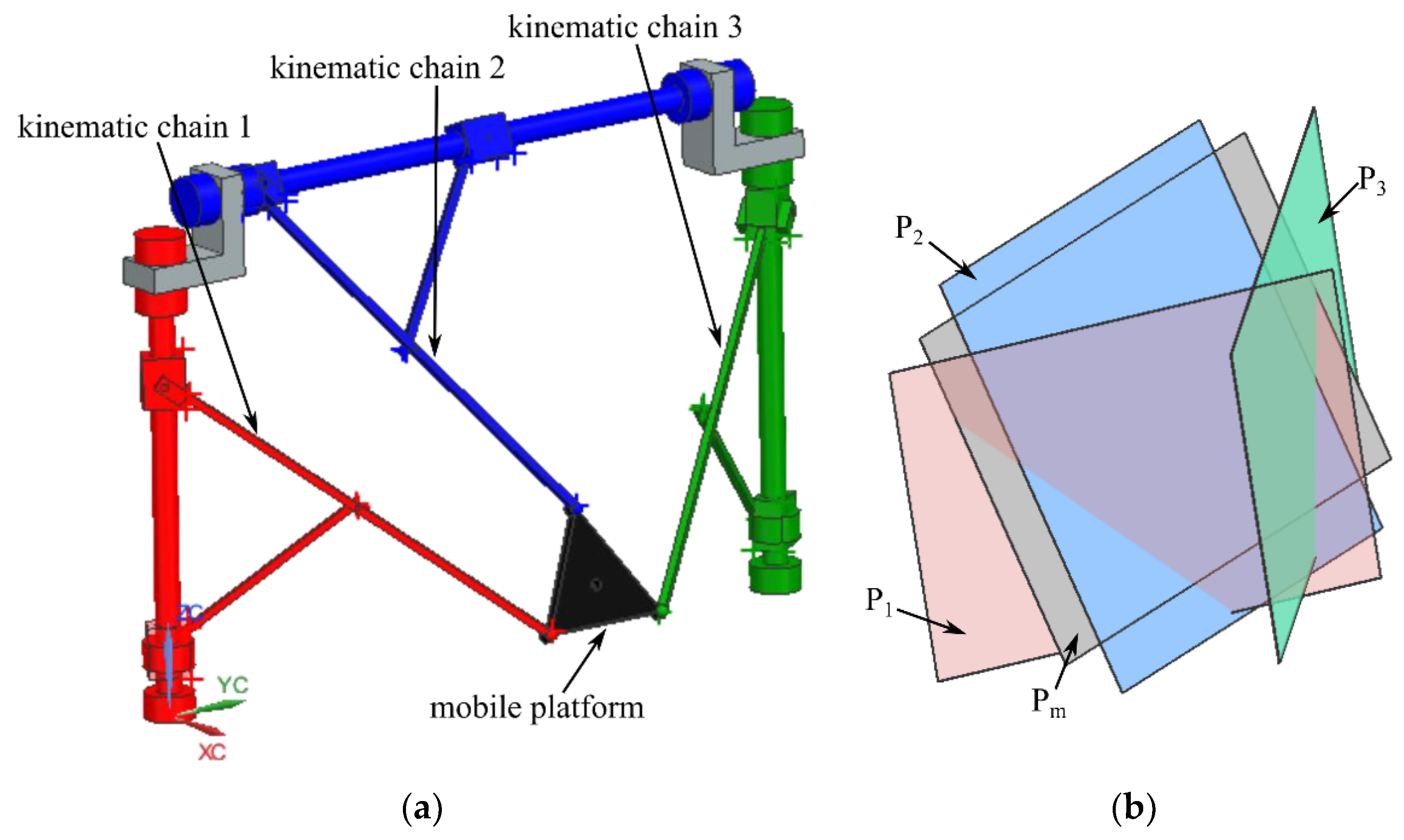
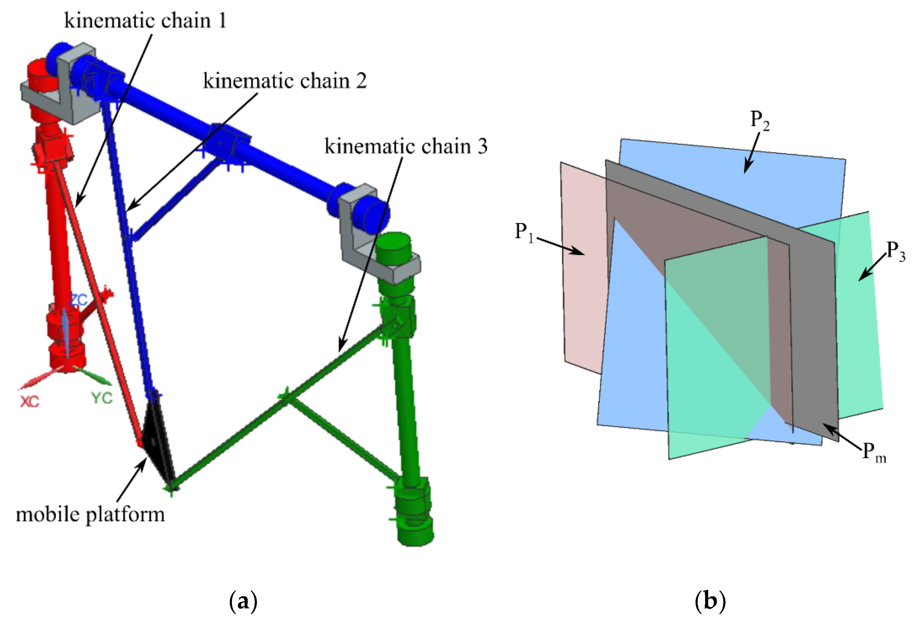
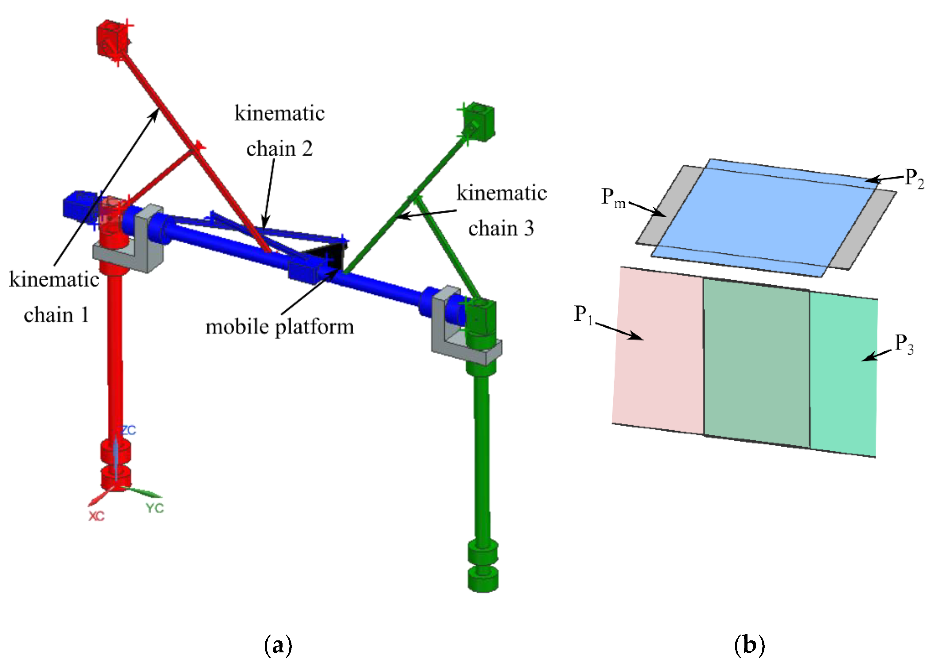
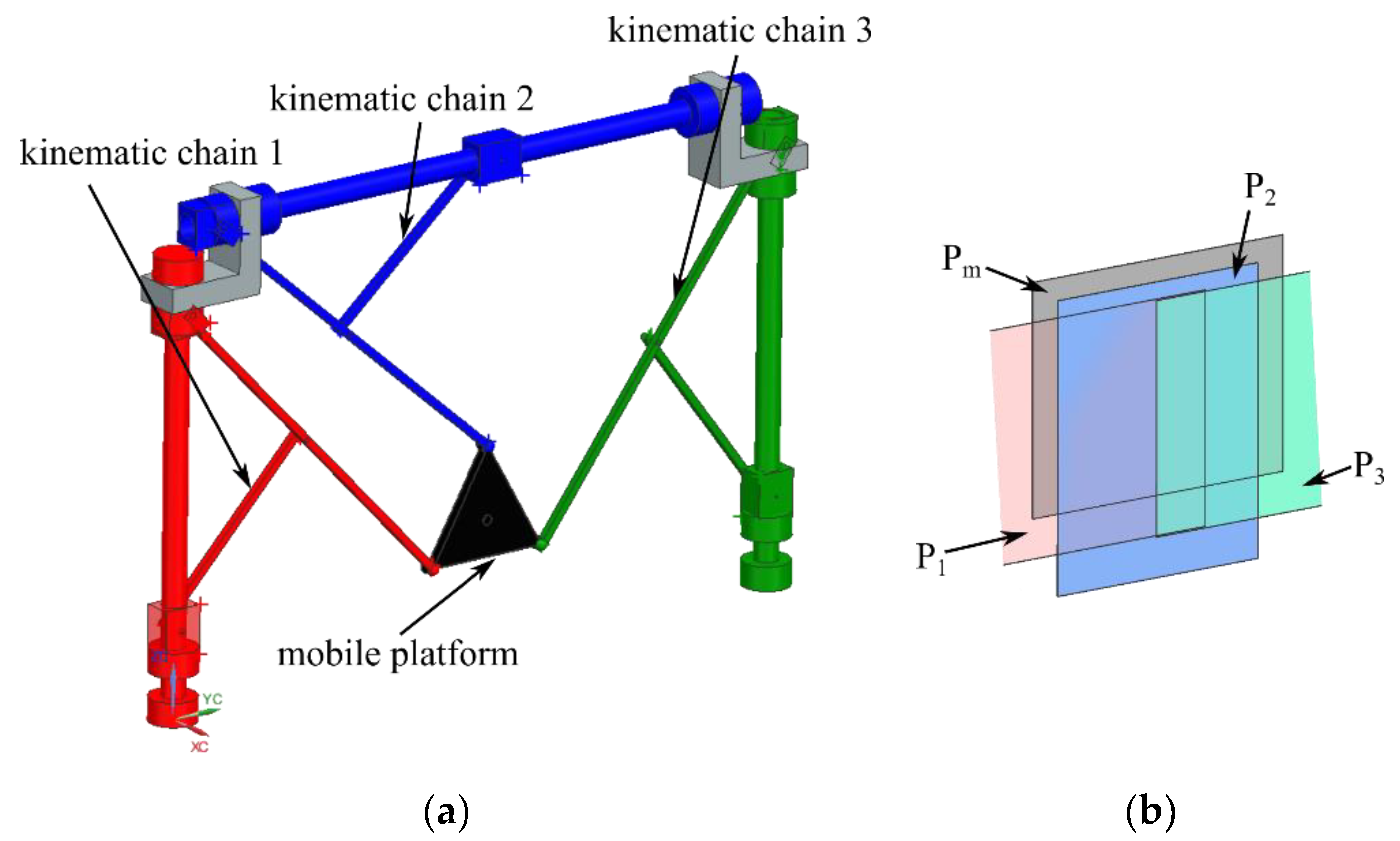
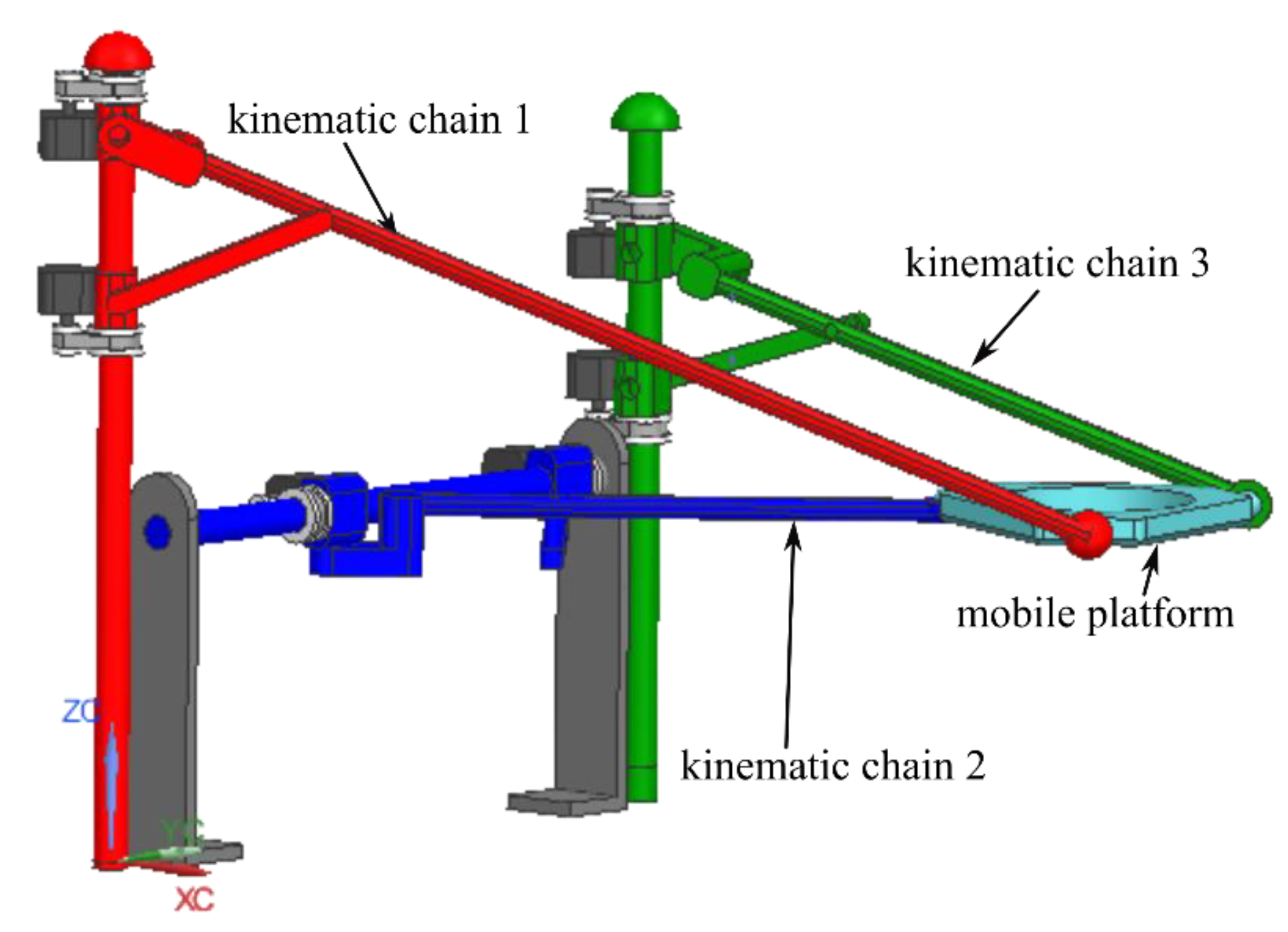
  • The parallel robot consists of three (R-PRR-PRS) kinematic chains actuated by the prismatic joints pairs q1 and q2 for the first kinematic chain, q3 and q4 for the second kinematic chain, and q5 and q6 for the third kinematic chain. Furthermore, each kinematic chain has a free rotation motion around the actuation axis of the prismatic joints (Rf1, Rf2, and Rf3, respectively), and three passive revolute joints (R11, R12, and R13 for the first kinematic chain, R21, R22, and R23 for the second kinematic chain, R31, R32, and R33 for the third kinematic chain);
  • The three kinematic chains guide the mobile platform via three passive spherical joints, S1, S2, and S3, respectively. The mobile platform contains two orientation platforms which are illustrated in Figure 2 (Detail 2) as generic mechanisms (to point out the functionality). The kinematic scheme of these orientation platforms is presented in [29];
  • The fixed coordinate frame OXYZ is attached to the robot base, and the mobile coordinate frame O’X’Y’Z’ is attached to the mobile platform with its origin at the geometric center of the equilateral triangle formed by the centers of the three passive spherical joints (S1, S2, S3). Furthermore, point E [XE, YE, ZE] is defined as the origin of the mobile coordinate frame O’X’Y’Z’.

Inverse Geometric Modelling for the 6-DOF Parallel Robot

The inverse geometric model will provide constraint equations which, in turn, will be used as objective functions for the optimization algorithm.
For the inverse geometric model, the inputs are the Cartesian coordinates of point E [XE, YE, ZE] and the orientation angles ψ, θ, φ, whereas the outputs are the active joint generalized coordinates qi (i = 1…6). With respect to the ZYX Euler convention, the coordinates of the passive spherical joints are:
S 1 : X S 1 = X E + 3 6 l p c ψ c θ 1 2 l p c ψ s θ s φ + 1 2 l p s ψ c θ Y S 1 = Y E + 3 6 l p s ψ c θ 1 2 l p s ψ s θ s φ 1 2 l p c ψ c θ Z S 1 = Z E 3 6 l p s θ 1 2 l p s φ c θ , S 2 : X S 2 = X E 3 3 l p c ψ c θ Y S 2 = Y E 3 3 l p s ψ c θ Z S 2 = Z E + 3 3 l p s θ , S 3 : X S 3 = X E + 3 6 l p c ψ c θ + 1 2 l p c ψ s θ s φ 1 2 l p s ψ c θ Y S 3 = Y E + 3 6 l p s ψ c θ + 1 2 l p s ψ s θ s φ + 1 2 l p c ψ c θ Z S 3 = Z E 3 6 l p s θ + 1 2 l p s φ c θ
where c ψ , c θ , c φ represent the cosines of the ψ, θ, φ Euler angles, and s ψ , s θ , s φ represent the sines of the ψ, θ, φ, Euler angles, respectively. Furthermore, the distances between S1, S2, S3 and the actuation axes of the three kinematic chains (Figure 2) are given by [27]:
R 1 = 1 2 l 1 l 1 + l 2 4 l 1 2 q 2 q 1 2 , R 2 = 1 2 l 1 l 1 + l 3 4 l 1 2 q 4 q 3 2 , R 3 = 1 2 l 1 l 1 + l 4 4 l 1 2 q 6 q 5 2
In addition, the following circle equation must be fulfilled [27]:
X S 1 2 + Y S 1 2 R 1 2 = 0 X S 2 2 + Z S 2 L V 2 R 2 2 = 0 X S 3 2 + Y S 3 L H 2 R 3 2 = 0
And the following equations derived for each kinematic chain of the 6-DOF parallel robot (Figure 2) must be fulfilled:
q 2 1 2 l 1 l 1 + l 2 q 2 q 1 Z S 1 = 0 q 4 + 1 2 l 1 l 1 + l 3 q 3 q 4 Y S 2 = 0 q 6 1 2 l 1 l 1 + l 4 q 6 q 5 Z S 3 = 0
Using Equations (1)–(3) yields the solution for the inverse geometric model:
q 1 = 1 l 1 + l 2 l 1 + l 2 q 2 2 l 1 X S 1 2 Y S 1 2 + l 1 + l 2 2 q 2 = l 1 + l 2 2 X S 1 2 Y S 1 2 + Z S 1 q 3 = 1 l 1 + l 3 l 1 + l 3 q 4 + 2 l 1 X S 2 2 + l 1 + l 3 2 L V Z S 2 2 q 4 = Y S 2 l 1 + l 3 2 X S 2 2 L V Z S 2 2 q 5 = 1 l 1 + l 4 l 1 + l 4 q 6 2 l 1 X S 3 2 + l 1 + l 4 2 L H Y S 3 2 q 6 = l 1 + l 4 2 X S 3 2 L H Y S 3 2 + Z S 3

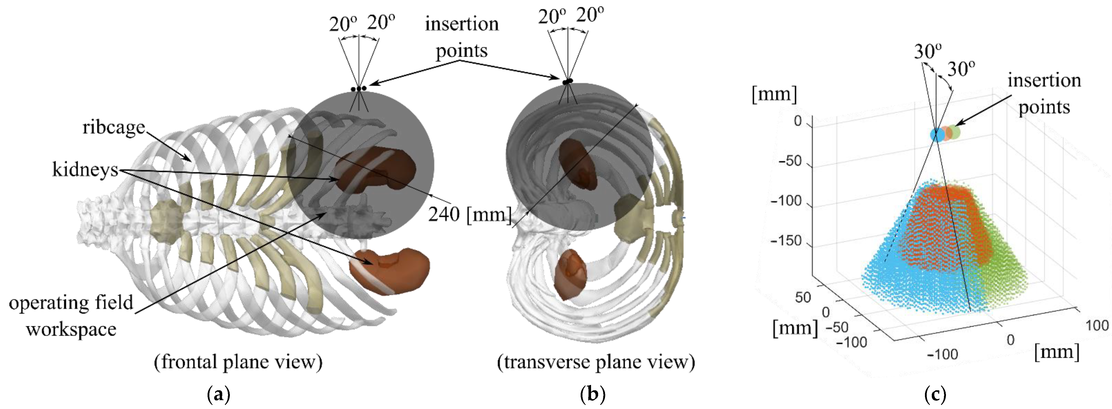
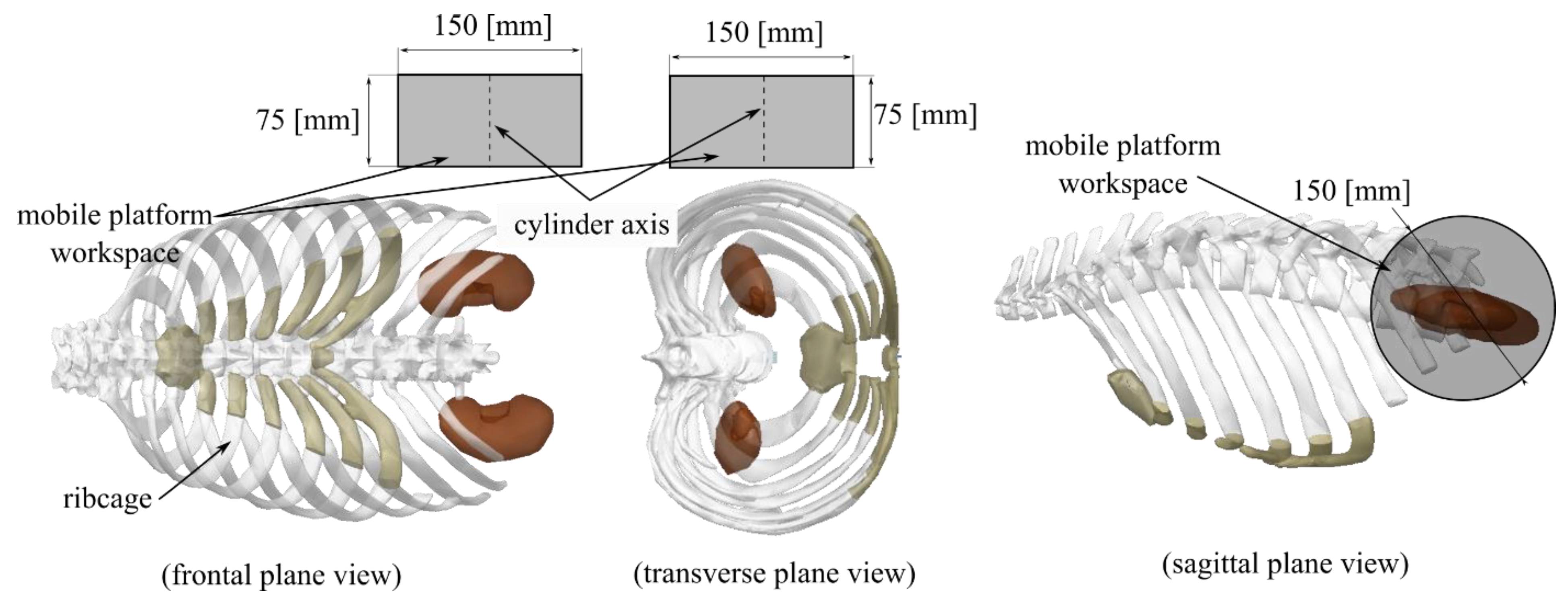
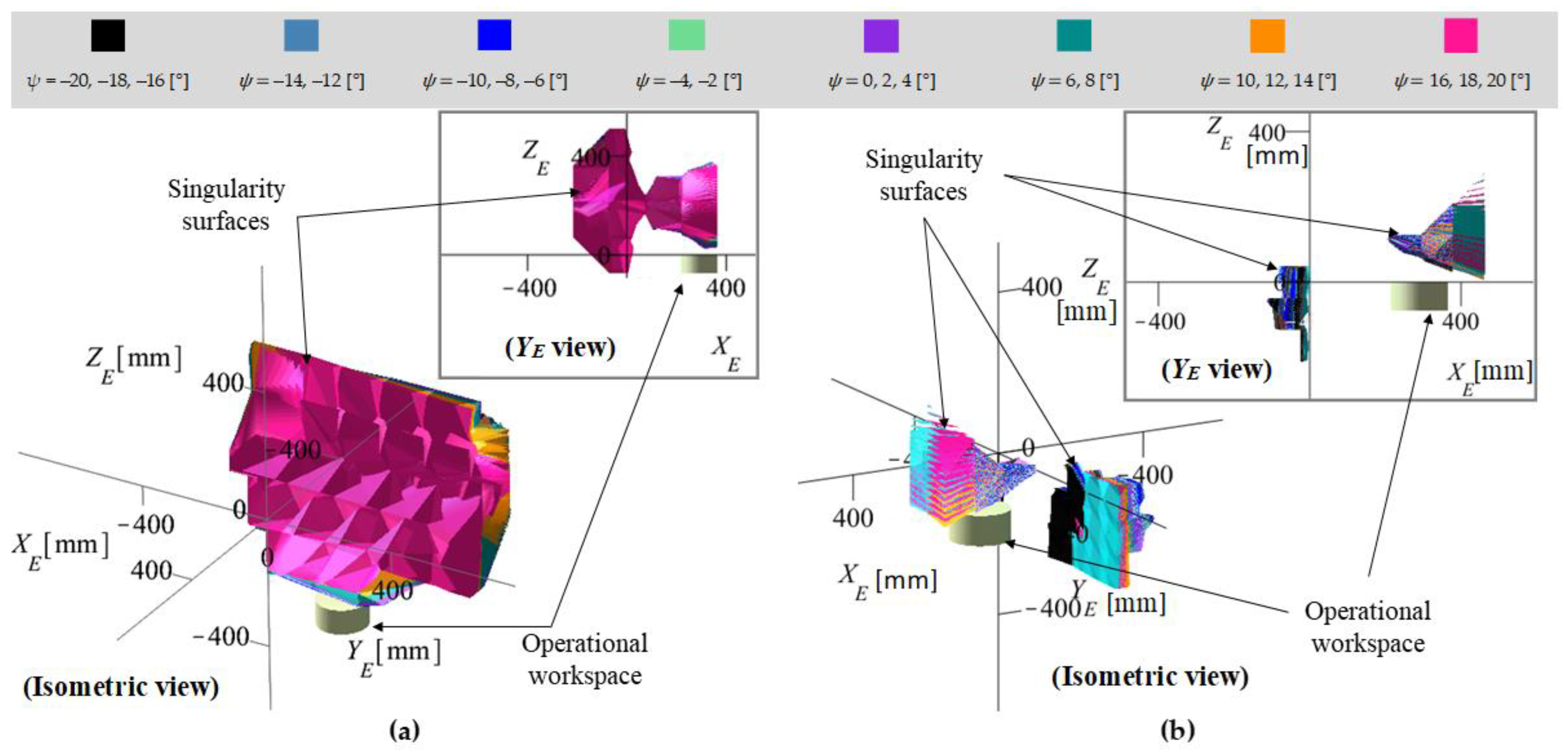
3. The Proposed Operational Workspace for the Parallel Robotic System for SILS

For the SILS task, the discussion of the operational workspace must be split into two components: (1) the intraoperative operational workspace (inside the patient body with respect to the insertion points), defined by the orientation platforms, the surgical instruments, and the mobile platform of the 6-DOF parallel robot (for the laparoscopic camera), and (2) the external operating workspace (outside the patient body with respect to the insertion points), defined only by the 6-DOF parallel robot.
Considering the intraoperative workspace, in previous work [29], the maximum values for the orientation angles of the surgical instruments were proposed as follows:
  • The maximum laparoscope angles in all directions with respect to a vertical axis passing through the insertion point to be 20 [°], achieved with the 6-DOF parallel robot;
  • The maximum angle for the active instruments in all directions with respect to an axis orthogonal to the mobile platform (of the 6-DOF parallel robot) passing through the insertion point to be 30 [°], achieved with the orientation platforms described in [29].
Larger angles may affect patient safety. The intraoperative workspace was defined based on a sphere of 240 mm in diameter. Figure 3 illustrates the proposed intraoperative workspace, showing possible insertion points for the surgical instruments and their maximum orientation angles
A single set of insertion points for the RCM motion is not sufficient since adjustments may be required for the relative position between the patient and the robot. Consequently, for the external operational workspace, a cylindrical volume was proposed that should contain the sets of insertion points. The proposed cylinder was defined with radius R = 75 [mm] and height h = 75 [mm], and its position (approximately) relative to the patient is shown in Figure 4. This cylinder represents the operational workspace of the 6-DOF parallel robot.

4. Singularities of the 3-R-PRR-PRS Parallel Robot

The singularity analysis is achieved for the 3-R-PRR-PRS parallel robot without the loss of generality (e.g., no numerical values will be substituted for the geometric parameters). Later in Section 5, the design solution for the 6-DOF parallel robot for SILS is selected (based on the 3-R-PRR-PRS parallel robot), and the singularities are correlated with the operational workspace for the SILS task.
The singularities are studied using the vanishing conditions of the determinants of the Jacobian matrices A and B from the matrix relation [33,34,35]:
A · X ˙ + B · Q ˙ = 0
where   Q ˙ and   X ˙ represent the velocity vectors for the active joints Q = q 1 , q 2 , q 3 , q 4 , q 5 , q 6 T and for the mobile platform coordinates X = X E , Y E , Z E , ψ , θ , φ T , respectively. With respect to the Jacobi matrices A and B, three types of singularities can be defined, namely: type I singularities (input singularities) when det(B) = 0, type II singularities (output singularities) when det(A) = 0, and type III singularities when both det(B) = 0 and det(A) = 0.
The implicit equations used in the singularity analysis were defined using Equations (3) and (4) with Equations (1) and (2) substituted, yielding:
f 1 : 1 6 l 1 l p l 1 3 s θ + 3 c θ s φ + 3 q 1 + q 2 2 Z E + 3 l 2 q 1 q 2 = 0 f 2 : 1 12 l 1 4 3 l 1 l p X E c ψ + Y E s ψ 1 2 l p s φ s θ c θ + l 1 l p 2 3 c φ 2 2 c θ 2 12 l 1 l p X E c ψ + Y E s ψ s φ s θ X E s ψ Y E c ψ c φ         12 l 1 2 l 1 + 2 l 2 + 12 l 1 X E 2 + Y E 2 l 2 2 + 3 l 1 l p 2 q 1 + q 2 2 + 6 l 2 q 1 q 2 2 + 3 l 2 2 l 1 q 1 q 2 2 = 0 f 3 : 1 6 l 1 2 3 l p l 1 s ψ c θ + 3 q 3 + q 4 2 Y E + 3 l 3 q 3 q 4 = 0 f 4 : 1 12 l 1 8 3 l 1 l p X E c ψ c θ + L V Z E s θ + 4 l 1 l p 2 3 c ψ 2 1 c θ 2 12 l 1 2 l 1 + 2 l 2 + 12 l 1 L V Z E 2 + X E 2 l 3 2 +       + l 1 4 l p 2 3 q 3 q 4 2 + 3 2 l 3 + l 3 2 l 1 q 3 q 4 2 = 0 f 5 : 1 6 l 1 l p l 1 3 s θ 3 s φ c θ + 3 q 5 + q 6 2 Z E + 3 l 4 q 5 q 6 = 0 f 6 : 1 12 l 1 4 3 l 1 l p L H Y E s ψ 1 2 l p s φ s θ X E c ψ c θ + l 1 l p 2 3 c φ 2 2 c θ 2 12 l 1 l p L H Y E s φ s θ + X E c φ +       + 12 l 1 l p X E s φ c ψ s θ ( L H Y E ) c ψ c θ 12 l 1 2 l 1 + 2 l 4 + 12 l 1 L H Y E 2 + X E 2 l 2 2 + 3 l 1 l p 2 + q 5 q 6 2 +       + 3 2 l 4 + l 4 2 l 1 q 5 q 6 2 = 0

4.1. Type I Singularities

Computing the determinant of the Jacobian Matrix B yields a factored result:
det ( B ) = 1 8 l 1 6 l 1 + l 2 2 l 1 + l 3 2 l 1 + l 4 2 q 1 q 2 q 3 q 4 q 5 q 6
The singularity analysis is as follows:
  • l 1 = 0 ; this condition causes det(B) to be undefined; however, this condition is disregarded since it will be avoided in the mechanism design (link lengths cannot be 0);
  • l 1 + l 2 = 0 or l 1 + l 3 = 0 or l 1 + l 4 = 0 ; these conditions imply negative values for the link lengths, and are not regarded as possible singularities due to the mechanism design;
  • q 1 q 2 = 0 or q 3 q 4 = 0 or q 5 q 6 = 0 ; these conditions require that the active joints of a kinematic chain are equal, meaning the active joints are overlapping. This condition is avoidable in the robot design or in the robot control.

4.2. Type II Singularities

Computing the determinant of the Jacobian matrix A yields a factored result:
det ( A ) = l p 3 cos ( θ ) F X E , Y E , Z E , ψ , θ , φ , l p , L H , L V
which describes singularities when:
  • l p = 0 , which is impossible in the robot design (link lengths cannot be zero);
  • cos ( θ ) = 0 , which describes a parametric singularity of the ZYX Euler angles; since the parameter θ describes the second rotation in the ZYX Euler angles, for θ = π/2 there is a gimbal lock, i.e., the parameters ψ and φ describe rotations about the same axis [36].
  • F X E , Y E , Z E , ψ , θ , φ , l p , L H , L V = 0 . The factor F (shown in Appendix A) could not be further factorized in this work. However, the following relation can be written:
det ( A ) = 8 H 0 cos θ
where the factor H0 (shown in Equation (11)) is written in a compact manner using Equation (1). Note that the lp parameter is not present in H0 (but is still encoded in Equation (1)).
H 0 = L H L V X S 2 Y S 2 X S 2 Y S 3 X S 3 Y S 2 + X S 3 Y S 3 X S 1 2 X S 1 Y S 1 X S 1 Y S 3 X S 2 2 X S 1 Y S 1 X S 1 Y S 2 X S 3 2 + + 2 Y S 1 Y S 2 Y S 3 X S 1 X S 2 X S 3 L H X S 2 Y S 2 Z S 3 X S 2 Y S 3 Z S 2 X S 3 Y S 2 Z S 2 + X S 3 Y S 3 Z S 2 X S 1 2 X S 1 Y S 1 Z S 3 X S 1 Y S 3 Z S 1 X S 3 Y S 1 Z S 1 + X S 3 Y S 1 Z S 3 X S 2 2 X S 1 Y S 1 Z S 2 X S 1 Y S 2 Z S 2 X S 2 Y S 1 Z S 1 + X S 2 Y S 1 Z S 2 X S 3 2 + + 2 Y S 1 Z S 2 Y S 2 Z S 3 Y S 3 Z S 1 X S 1 X S 2 X S 3 L V X S 2 Y S 2 Y S 3 X S 2 Y S 3 2 X S 1 2 X S 1 Y S 1 Y S 3 + X S 3 Y S 1 Y S 3 X S 1 Y S 3 2 X S 3 Y S 1 2 X S 2 2 + X S 2 Y S 1 Y S 2 X S 2 Y S 1 2 X S 3 2 + 2 Y S 1 Y S 3 Y S 1 Y S 2 Y S 2 Y S 3 X S 1 X S 2 X S 3 + + Y S 2 Y S 3 Z S 3 Y S 3 2 Z S 2 X S 1 2 X S 2 Y S 1 Y S 3 Z S 3 Y S 3 2 Z S 1 X S 2 2 X S 1 Y S 1 Y S 2 Z S 3 2 Y S 1 Y S 3 Z S 2 + Y S 2 Y S 3 Z S 1 X S 1 X S 2 X S 3 Y S 1 Y S 3 Z S 1 Y S 1 2 Z S 3 X S 2 2 X S 3 + Y S 1 Y S 2 Z S 1 Y S 1 2 Z S 2 X S 3 2 X S 2
To study the output singularities, the characteristic tetrahedron was used [30], which states that a singularity occurs when the geometry of the tetrahedron is degenerate (e.g., faces are coplanar, etc.). The tetrahedron is composed of three faces defined by characteristic planes spanned by reciprocal wrenches at each spherical joint of the three kinematic chains and a base defined by the plane of the mobile platform. To define the characteristic planes associated with the three kinematic chains (for the 6-DOF parallel robot for SILS), first, the actuators are considered fixed, and then two reactive forces for the remaining passive motion are defined (at the level of the spherical joint). Figure 5 illustrates this concept on the kinematic chain 1, with the actuators q1 and q2, the spherical joint S1, and the reactive forces R1 and R2, respectively (which span the characteristic plane P1). Figure 6 illustrates how these planes intersect to form the characteristic tetrahedron (in a nonsingular pose).
The first characteristic plane, P1 (describing the first kinematic chain), contains the OZ axis (the actuation axis of q1 and q2) of the fixed coordinate system and the center of the passive spherical joint S1 and has the following equation:
P 1 : Y S 1 x + X S 1 y = 0
Furthermore, the characteristic plane P2 (for the second kinematic chain) contains the actuation axis of q3 and q4 and the center of the passive spherical joint S2 and has the following equation:
P 2 : Z S 2 L V x X S 2 z + L V X S 2 = 0
The characteristic plane P3 (for the third kinematic chain) contains the actuation axis of q5 and q6 and the center of the passive spherical joint S3 and has the equation:
P 3 : Y S 3 + L H x + X S 3 y L H X S 3 = 0
Lastly, the characteristic plane Pm (for the mobile platform) contains the centers of all passive spherical joints and has the equation:
          P m : C o e f x x + C o e f y y + C o e f z z + C o e f d = 0 C o e f x = Z S 2 Z S 3 Y S 1 + Z S 3 Z S 1 Y S 2 + Z S 1 Z S 2 Y S 3 C o e f y = Z S 3 Z S 2 X S 1 + Z S 1 Z S 3 X S 2 + Z S 2 Z S 1 X S 3 C o e f z = Y S 2 Y S 3 X S 1 + Y S 3 Y S 1 X S 2 + Y S 1 Y S 2 X S 3 C o e f d = X S 2 Y S 1 X S 1 Y S 2 Z S 3 + Y S 2 Z S 1 Y S 1 Z S 2 X S 3 + X S 1 Z S 2 X S 2 Z S 1 Y S 3
There are eight type II (output) singularities (described in a general form in [30]) that are geometrically interpreted by the degeneracy of the geometry of the characteristic tetrahedron. Each singularity case for the 3-R-PRR-PRS parallel robot may be checked independently using the planes defined in Equations (12)–(15) (the planes contain the faces and the base of the characteristic tetrahedron) and Equation (11), which generally describes the degeneracy conditions of the characteristic tetrahedron:
In Case 1, all faces of the characteristic tetrahedron and the base intersect in a point [30]; consequently, P1, P2, P3, and Pm intersect in a point. The proof that this case represents a singularity for the 3-R-PRR-PRS parallel robot is straightforward. Assuming that the characteristic planes P1, P2, P3, intersect at point I(x, y, z). Equations (12)–(14) can be solved simultaneously to compute the intersection point’s Cartesian coordinates:
I : x = L H X S 1 X S 3 L H Y S 3 X S 1 + X S 3 Y S 1 y = L H X S 3 Y S 1 L H Y S 3 X S 1 + X S 3 Y S 1 z = L H L V X S 1 X S 2 X S 1 X S 3 + L V X S 2 X S 3 Y S 1 X S 1 X S 2 Y S 2 + L H X S 1 X S 3 Z S 2 L H Y S 3 X S 1 + X S 3 Y S 1 X S 2
If point I is also contained in the characteristic plane Pm, then Equation (15) must be fulfilled for the x, y, and z Cartesian components shown in Equation (16). Substituting Equation (16) into Equation (15) leads to an equation that can be linearly solved for one Cartesian component of the three passive spherical joints. The computed solution for ZS1 is:
Z S 1 = H 1 L H Y S 3 X S 2 L H Y S 2 X S 3 X S 1 Y S 3 X S 3 Y S 1 X S 2 H 1 = L H L V X S 2 X S 3 Y S 3 Y S 1 X S 1 + Y S 2 Y S 3 X S 2 + Y S 1 Y S 2 X S 3 X S 1 L H Z S 2 Y S 3 Y S 2 X S 2 + Y S 2 Z S 3 Y S 3 Z S 2 X S 3 X S 1 2 + Z S 2 Y S 2 Y S 1 X S 3 2 + + X S 2 2 Y S 1 Z S 2 Y S 2 Z S 3 X S 3 X S 2 2 Y S 1 Z S 3 X S 1 + X S 2 Z S 3 X S 3 Z S 2 X S 2 X S 3 Y S 1 L V Y S 2 Y S 3 X S 1 + Y S 3 Y S 1 X S 3 + Y S 1 Y S 2 X S 3 X S 1 Y S 3 X S 3 Y S 1 X S 2 + + Y S 2 Z S 3 Y S 3 Z S 2 X S 1 X S 2 Z S 3 X S 3 Z S 2 Y S 1 X S 1 Y S 3 X S 3 Y S 1 X S 2
Equation (17) describes the constraint of the ZS1 parameter when all four planes intersect at a point. Substituting Equation (17) into Equation (11) causes H0 to vanish, proving the singularity for the 3-R-PRR-PRS parallel robot.
To illustrate an example of this singularity, the geometric parameters {LH = 1420, LV = 1000, lp = 260} [mm] and the mobile platform coordinates {XE = 400 mm, YE = 700 mm, ZE = 500 mm, ψ = 0 rad, φ = π/10 rad} (arbitrary chosen) are considered (only five output parameters are considered, the last one, θ, is computed). Substituting the numerical values into Equation (A1) (see Appendix A) and solving the equation for θ (using the solve function in Maple), yields four real solutions {θ = 0.93 rad, θ = −1.755 rad, θ = 1.82 rad, θ = −2.40 rad}. Figure 7a shows the parallel robot in the singular pose (for θ = 0.93), whereas Figure 7b shows how the characteristic planes P1, P2, P3, and Pm intersect at a point.
In Case 2, the faces of the characteristic tetrahedron (i.e., P1, P2, P3) intersect in a line, but no faces are coplanar [30]. For the 6-DOF parallel robot for SILS, this case is impossible since P1 and P3 are always vertical, whereas P2 has only two configurations when it is vertical (when the kinematic chain 2 points upwards or downwards). However, when all of the characteristic planes, P1, P2, and P3, are vertical, they are all coplanar (due to the mechanism topology); therefore, P1, P2, and P3 cannot intersect in a line. This is straightforward to prove using Equations (12)–(14). Assuming that the planes P1, P2, and P3 intersect in a line, then the rank of the coefficient’s matrix (matrix containing the x, y, and z coefficients from the plane equations) M1 and the rank of the augmented matrix (matrix containing the x, y, and z coefficients and the free terms) M2 must be 2. The two matrices are defined using Equations (12)–(14):
M 1 : Y S 1 X S 1 0 L V + Z S 2 0 X S 2 L H Y S 3 X S 3 0 ,   M 2 : Y S 1 X S 1 0 0 L V + Z S 2 0 X S 2 L V X S 2 L H Y S 3 X S 3 0 L H X S 3
It can be checked that the rank of M1 is 2 for:
X S 2 = 0 ,   and / or   X S 1 = Y S 1 X S 3 Y S 3 L H
but for the solutions shown in Equation (18a) the rank of M2 is 3 (the planes intersect in two or three lines). The rank of M2 is 2 for:
X S 2 = 0 ,   and   X S 1 = 0
in which case the rank of M1 is also 2 (describing two coincident planes and the third one intersecting it). Furthermore, for:
X S 2 = 0 ,   and X S 1 = 0 ,   and   X S 3 = 0
the rank of both M1 and M2 is 1 (describing three coincident planes).
In Case 3, two of the tetrahedron faces and its base intersect in a line [30]. Considering the characteristic planes P1, P3, and Pm, the coefficient and augmented matrices are:
M 3 : Y S 1 X S 1 0 L H Y S 3 X S 3 0 C o e f x C o e f y C o e f z ,   M 4 : Y S 1 X S 1 0 0 L H Y S 3 X S 3 0 L H X S 3 C o e f x C o e f y C o e f z C o e f d
It can be checked that the rank of both matrices M3 and M4 is 2 for:
X S 1 = X S 3 Y S 1 Y S 3 ,   and   X S 2 = X S 3 Y S 2 Y S 3
Furthermore, substituting the values of Equation (20) into Equation (19) shows no proportionality between the matrix’s rows; therefore, the intersection describes a line. In addition, substituting Equation (20) into Equation (11) causes the factor H0 to vanish.
Another geometric configuration for Case 3 is represented by the characteristic planes P1, P2, and Pm intersecting in a line (the case when P3, P2, and Pm intersect in a line is redundant with this one due to the configuration symmetry of the parallel robot). The coefficient and augmented matrices are:
M 5 : Y S 1 X S 1 0 L V + Z S 2 0 X S 2 C o e f x C o e f y C o e f z ,   M 6 : Y S 1 X S 1 0 0 L V + Z S 2 0 X S 2 L V X S 2 C o e f x C o e f y C o e f z C o e f d
The rank of both matrices M5 and M6 is 2 for:
X S 1 = X S 3 L V Z S 1 L V Z S 3 ,   and X S 2 = X S 3 L V Z S 2 L V Z S 3
Substituting the values of Equation (20a) into Equation (20) shows no proportionality between the matrix’s rows (the intersection describes a line), and substituting Equation (20a) into Equation (11) causes factor H0 to vanish.
As an example, for the 3-R-PRR-PRS parallel robot, for θ = 0 rad, φ = π/2 rad, the factor F (Equation (A1)—Appendix A) vanishes. In this configuration, the mobile platform is in a vertical pose. Figure 8 shows an example of this singularity, (a) the parallel robot poses and (b) the characteristic planes (P1, P3, Pm) intersecting in a line. It can be shown (at least for this example) that the characteristic plane P2 also intersects that line; therefore, this singularity is the special case of Case 1 discussed previously (since all the characteristic planes intersect at a point).
In Case 4, two of the characteristic tetrahedron faces are coplanar [30]. Due to the arguments presented in Case 2 for the 6-DOF parallel robot for SILS, the only possible tetrahedron faces that can become coplanar are the ones defined by P1 and P3. The coefficient and augmented matrices in this case are:
M 7 : Y S 1 X S 1 0 L H Y S 3 X S 3 0 ,   M 8 : Y S 1 X S 1 0 0 L H Y S 3 X S 3 0 L H X S 3
If P1 and P3 are coplanar then the ranks of M7 and M8 must both be 1. It can be checked that this is the case for:
X S 1 = 0 ,   and X S 3 = 0
Substituting Equation (21a) into Equation (11) causes factor H0 to vanish, proving the singularity. As an example, for the numerical values X E = 3 6 l p mm, ψ = 0 rad, θ = 0 rad, the factor F vanishes. Figure 9a shows this singular configuration for the parallel robot, and Figure 9b shows P1 and P3 being coplanar.
In Case 5, one side and the base of the characteristic tetrahedron are coplanar [30]. There are three general configurations for the 3-R-PRR-PRS parallel robot that correspond to this case. The first of these general configurations is represented by P2 and Pm being coplanar, whereas the second and third general configurations for this singularity are achieved when either P1 or P2 are coplanar with Pm. Considering the first case, the coefficient and augmented matrices are:
M 9 : L V + Z S 2 0 X S 2 C o e f x C o e f y C o e f z ,   M 10 : L V + Z S 2 0 X S 2 L V X S 2 C o e f x C o e f y C o e f z C o e f d
It can be shown that both matrices M9 and M10 have rank 1 for:
                        X S 2 = Y S 2 Y S 3 X S 1 + Y S 1 Y S 2 X S 3 Y S 1 Y S 3 ,   and   Z S 1 = Y S 1 Y S 3 Z S 2 + Y S 2 Y S 1 Z S 3 Y S 2 Y S 3
Substituting Equation (22a) into Equation (11) causes factor H0 to vanish. It is easy to find relationships that describe this singularity case when P1 or P2 are coplanar with Pm.
An example is given for the geometric parameters {LH = 1420 mm, LV = 1000 mm, lp = 260 mm}, and for the mobile platform coordinates {XE = 350 mm, YE = 750 mm, ZE = 200 mm, ψ = 0 rad, φ = 0 rad} (arbitrary chosen for the example purpose). Solving the factor F for the numerical values yields two real solutions {θ = 1.158 rad, θ = 1.9 rad}. Figure 10 illustrates this singularity for θ = 1.158 rad. Another example is shown for the mobile platform coordinates {XE = 350 mm, YE = 750 mm, ZE = 200 mm, ψ = 0 rad, θ = π/2 rad} and the computed angle for φ = 0.44 rad. In this example (Figure 11) P1 and Pm are coplanar.
In Case 6, two sides and the base of the characteristic tetrahedron are coplanar [30]. For the 6-DOF parallel robot for SILS this case is impossible (due to the mechanism topology). Any two faces of the characteristic tetrahedron are coplanar if and only if the faces are also coplanar with the YOZ plane (Figure 2). This condition can be proven in two steps. In the first step, P1, P3, and Pm are assumed to be all coplanar. Consequently, the ranks of M3 and M4 (Equation (19)) must both be 1, which can be achieved if:
X S 1 = 0 ,   and   X S 2 = 0 ,   and X S 3 = 0
It can be checked that Equation (23) is the only solution for which P1, P3, and Pm are all coplanar. This is also easy to see geometrically. The actuation axes of q1 and q2 (line contained in P1) and q5 and q6 (line contained in P3) are both included in the YOZ plane of the fixed coordinate system. If P1 and P3 are coplanar, then the actuation axis of q1 and q2 must be contained in P3, and reciprocally, the actuation axis of q5 and q6 must be contained in P1. Therefore, the planes P1 and P3 (and any other plane, e.g., Pm) are coplanar if they are coplanar with YOZ, the result is shown by Equation (23). In the second step, P1, P2, and Pm are assumed to be all coplanar. Consequently, the ranks of M5 and M6 (Equation (20)) must both be 1, which can be achieved if (again) the conditions from Equation (23) are met. It can be shown, by the same argument as above, that if the planes P1, P2, and Pm are coplanar, then they must be coplanar with YOZ, the result is shown by Equation (23). Since Equation (23) represents a (unique) solution for both cases (P1, P3, and Pm being coplanar and P1, P2, and Pm being coplanar), the conclusion is that if P1, P3, and Pm are coplanar, they must also be coplanar with P2 (condition discussed in Case 8).
In Case 7, one side and the base of the tetrahedron are coplanar and the other two sides of the tetrahedron are also coplanar [30]. Considering all four characteristic planes, the coefficient and augmented matrices are:
M 11 : Y S 1 X S 1 0 L V + Z S 2 0 X S 2 L H Y S 3 X S 3 0 C o e f x C o e f y C o e f z ,   M 12 : Y S 1 X S 1 0 0 L V + Z S 2 0 X S 2 L V X S 2 L H Y S 3 X S 3 0 L H X S 3 C o e f x C o e f y C o e f z C o e f d
The ranks of the matrices M11 and M12 is 2 (describing pairs of coplanar planes that intersect in a line), for:
X S 1 = 0 ,   and X S 3 = 0 ,   and   Z S 1 = L V ,   and   Z S 3 = L V
Substituting Equation (26) in Equation (11) causes H0 to vanish.
For the 3-R-PRR-PRS parallel robot, this case can only be achieved if P1 is coplanar with P3 and P2 is coplanar with Pm. The factor F vanishes for the geometric values parameters {LH = 1420 mm, LV = 1000 mm, lp = 260 mm}, and for the mobile platform coordinates {XE = −75.05 mm, YE = 750 mm, ZE = 1000 mm, ψ = 0 rad, θ = 0 rad, φ = 0 rad}. This configuration is illustrated in Figure 12.
In Case 8, all of the faces and the base of the characteristic tetrahedron are coplanar [30]. The coefficient and augmented matrices for this case are already shown in Equation (24). All four planes are coplanar if the ranks of the matrices M11 and M12 are both 1. This is achieved by setting:
X S 1 = 0 ,   and   X S 2 = 0 ,   and X S 3 = 0
Substituting Equation (25) into Equation (11) causes factor H0 to vanish. For the 3-R-PRR-PRS parallel robot, this singularity is achieved if {XE = 0 mm, θ = ±π/2 rad}. This configuration is illustrated in Figure 13.

4.3. Type III Singularities

Since the determinant of the Jacobian matrix A is free of input parameters (i.e., it only depends on the geometric parameters and the outputs {XE, YE, ZE, ψ, θ, φ}), whereas the determinant of the Jacobian matrix B is free of output parameters (it depends only on the geometric parameters and the inputs {q1, q2, q3, q4, q5, q6}), it is feasible to assume that type III singularities may occur. However, as stated before, the type I singularities are easily avoidable in the design stage; hence it can be stated that the 6-DOF parallel robot for SILS will have no type III singularities.

5. Geometric Optimization Algorithm

The 6-DOF parallel robot for SILS was geometrically optimized with respect to an operational workspace defined to comply with the medical task. Several optimization criteria were defined, and based on these criteria, appropriate input data were defined for the optimization algorithm.

5.1. Optimization Criteria

The following criteria (with the following importance order Criterion 1 is more important than Criterion 2, which is equally important as Criterion 3) were defined with respect to the SILS task:
  • Criterion 1—Operational workspace. The proposed operational workspace is a cylinder shape (see Section 3). Furthermore, the intervals for the orientation angles of the endoscopic camera must be (for the entire operational workspace):
ψ , θ , φ 20   20 °
  • Criterion 2—Footprint. To minimize the robot footprint, the following conditions were imposed:
L H < 600   [ mm ] ,   L V < 600   [ mm ]
  • Criterion 3—Dexterity. The robot should have adequate performance with respect to dexterity. This work uses an approximation of the Global Conditioning Index (GCIa) to assess the 6-DOF parallel robot dexterity which is computed as [16]:
GCI a = i = 1 n 1 k i n
where ki represents the condition number [16] of the ith point from the (discrete generated) operational workspace, which is computed using Equation (29), and n is the number of points within the operational workspace. For a given point, the condition number is:
k =   J     J 1
where   ·     represents the norm of the Jacobian matrix J, which is computed in this work with:
  J = trace J J T
where J is computed using the input and output Jacobian matrices (Equation (6)), as follows:
J = B 1 · A
An important note is that condition number k is a measure of dexterity at one specific robot configuration, and the lower its value, the better (a minimum value of 1 represents isotropy [16]). For the approximation of GCI, the inverse of k is used, which is bounded by 0 and 1 (in this case the higher the better). GCIa is a measure of the average of the inverse of k computed from all points within the operational workspace. However, due to the drawbacks of the condition number and the GCI (when the robot has translation and rotational motions), the values of GCIa (i.e., Criterion 3) will be used as a guiding value, not as a definite decision parameter.

5.2. Geometric Optimization Algorithm Description

The optimization algorithm is presented next in pseudocode (Algorithm 1).
Algorithm 1. The optimization algorithm.
0. 
BEGIN OPTIMIZATION
1. 
Define the test operational workspace
1.1.
Input the cartesian coordinates E(N) [XEi, YEi, ZEi] (i = 1,…,n) for the operating workspace
1.2.
Input the required orientation angles ψ, θ, φ
1.3.
Compute WS_DATA by assigning all angles ψ, θ, φ for all E(i) ∈ E(N)
1.4.
Goto2
2. 
Define objective functions and constraints
2.1.
Define objective functions OBJ [o1, o2, o3, o4, o5, o6, o7]
2.2.
Define constraints: C [C1, C2, C3, h1, h2, h3, h4, h5, h6]
2.3.
Goto3
3. 
Input the dimension intervals for the optimization process
3.1.
Define and input L [lp_min, lp_max, LH_min, LH_max, LV_min, LV_max, l1_min, l1_max, l2_min, l2_max, l3_min, l3_max, l4_min, l4_max]
3.2.
Define and input CYL [R_min, R_max, H_min, H_max, α_min, α _max]
3.3.
Define and input ANG [ψ_min, ψ _max, θ_min, θ _max, ϕ_min, ϕ _max]
3.4.
Goto4
4. 
Minimize robot dimensions
4.1.
Compute the Pareto front (iteratively) denoted SOLS(M) by minimizing OBJ subject to the constraints C and the intervals L, CYL, ANG.
4.2.
Define a smaller solution set SOL(K) ∈ SOLS(M) such that for every SOL(i) (i = 1,…,K), qi (i = 1,…,6) ∈ ℝ for every point in WS_DATA
4.3.
IfSOL(K) exists, then Goto 4.4, else Goto 3
4.4.
Compute the active joints ranges Q_RANGE(K) [qi_min, qi_max] (i = 1,…,6) for every SOL(i) (i = 1,…,K)
4.5.
IfQ_RANGE(j) (j = 1,…,K) is acceptable (mechanism is feasible), then save the solution SOL(j) into FINAL(H)
4.6.
IfFINAL(H) is empty, then Goto 3, else Goto 4.7
4.7.
Compute GCI for every FINAL(h) (h = 1,…,H)
4.8.
Define the most optimal solution
4.9.
Goto5
5. 
END OPTIMIZATION
The test operational workspace WS_DATA is defined (1) and is used in future steps to determine the validity of the possible optimized solutions. Note that the proposed algorithm yields solutions (stacked in SOLS(M)) for a single parallel robot pose (Cartesian coordinates and orientation) within the desired cylindrical operational workspace. These solutions must be subsequently validated for the entire WS_DATA. The objectives OBJ of optimization (2) are to minimize the seven geometric parameters of the parallel robot subject to the kinematic constraint C, which are evaluated with values for the mobile platform coordinates within the operational workspace. The numerical intervals for the optimization process are defined (3); L defines intervals for the robot geometric parameters (for the optimization objectives), whereas CYL ensures that the Cartesian coordinates (for the optimum solutions) are within the desired cylinder, and ANG ensures that the mobile platform orientations are within the proper ranges. Note, CYL and ANG are different from WS_DATA; CYL and ANG are used by the gamultiobj function (from Matlab [31]) to ensure that the objectives are always minimized with respect to robot poses within the operational workspace, whereas (as pointed out before) WS_DATA is used to evaluate (in a discrete manner) if the generated solutions are valid for the entire operational workspace. The optimization is performed (4) iteratively until the solutions set SOLS(M) fills as best as possible the operational workspace (considering, of course, the Cartesian coordinates and the orientations of the mobile platform). Then, a solution subset SOL(K) (for the minimized geometric parameters) is defined for the optimized solutions that are valid for the entire WS_DATA (i.e., geometric parameters that yield real solutions for all WS_DATA). If no such subset exists, (3) is repeated. Then, the solution subset is analyzed to determine the ranges of motion Q_RANGE(K) for the active joints qi (i = 1,…,6) and if there exist ranges that yield feasible mechanisms (without crossing the actuation axes of the active joints, etc.), the solutions (yielding the adequate ranges) are subsequently saved in FINAL(H). If there are no adequate ranges for the active joints (to yield feasible mechanisms), (3) is repeated. The GCI is computed for all of the remaining solutions in FINAL(H), and the design solution is defined (not automatically but by the robot designers).

6. The Optimized 6-DOF Parallel Robot for SILS

6.1. The Geometric Optimization

The parallel robot was optimized using the algorithm presented in Section 5.2 based on the following inputs:
  • The test workspace data (WS_DATA) was defined based on a cylinder with:
C X C = 290 , Y C = 415 , Z C = 75   [ mm ] R = 75   [ mm ] , h = 75   [ mm ]
where C is the center of the base circle (with respect to the fixed coordinate system of the robot), R is the circle’s radius, and h is the cylinder height. WS_DATA was generated by discretizing the cylinder and adding the orientations for the mobile platform, based on the following:
E i = X E i = X C + R C cos ( α ) Y E i = Y C + R C sin ( α ) Z E i = H C ψ i = ψ θ i = θ φ i = φ , R C 0 , 75 [ mm ] , increment = 7.5   [ mm ] H C 75 , 0 [ mm ] , increment = 15   [ mm ] α 0 , 360 [ ° ] , increment = 10   [ ° ] ψ , θ , φ 20 , 20 [ ° ] , increment = 2.5   [ ° ]
where Ei represents the ith mobile platform configuration within the operational workspace. WS_DATA contained approximately 9.78 million unique sets of mobile platform coordinates (a better resolution was not achievable due to computation power limitations). Figure 14 illustrates the point cloud defining the discrete operational workspace (only in Cartesian coordinates).
  • The input intervals L for the geometric parameters for the 6-DOF SILS robot where:
l 1 140 , 200 [ mm ] , l 2 350 , 600 [ mm ] , l 3 200 , 350 [ mm ] , l 4 200 , 350 [ mm ] , l p 200 , 250 [ mm ] , L H 500 , 600 [ mm ] , L V 200 , 600 [ mm ]
Furthermore, the CYL intervals were:
R 0 , 75 [ mm ] , H 75 , 0 [ mm ] , α 0 , 360 [ ° ]
and the ANG intervals:
ψ 20 , 20 [ ° ] , θ 20 , 20 [ ° ] , φ 20 , 20 [ ° ]
  • The objective functions OBJ to be minimized (to reduce the size of the robot for a given operational workspace) and the constraints C were:
OBJ = [ l p , L H , L V , l 1 , l 2 , l 3 , l 4 ] , C = [ X E , Y E , Z E , h 1 , h 2 , h 3 , h 4 , h 5 , h 6 ]
where hi (i = 1,…,6) are due to Equation (5):
h 1 : 1 l 1 + l 2 l 1 + l 2 q 2 2 l 1 X S 1 2 Y S 1 2 + l 1 + l 2 2 q 1 = 0 h 2 : l 1 + l 2 2 X S 1 2 Y S 1 2 + Z S 1 q 2 = 0 h 3 : 1 l 1 + l 3 l 1 + l 3 q 4 + 2 l 1 X S 2 2 + l 1 + l 3 2 L V Z S 2 2 q 3 = 0 h 4 : Y S 2 l 1 + l 3 2 X S 2 2 L V Z S 2 2 q 4 = 0 h 5 : 1 l 1 + l 4 l 1 + l 4 q 6 2 l 1 X S 3 2 + l 1 + l 4 2 L H Y S 3 2 q 5 = 0 h 6 : l 1 + l 4 2 X S 3 2 L H Y S 3 2 + Z S 3 q 6 = 0
and:
X E = X C + R cos ( β ) , Y E = Y C + R sin ( β ) , Z E = H
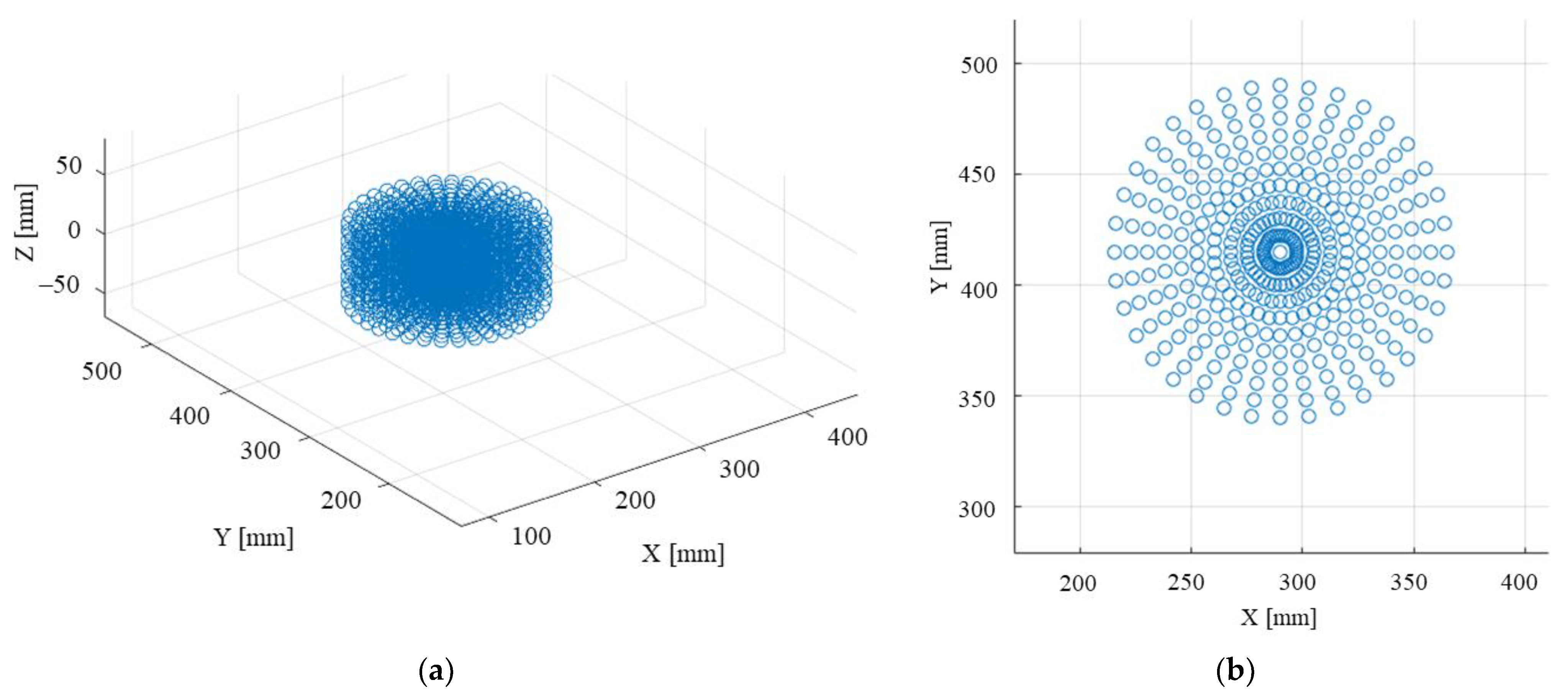
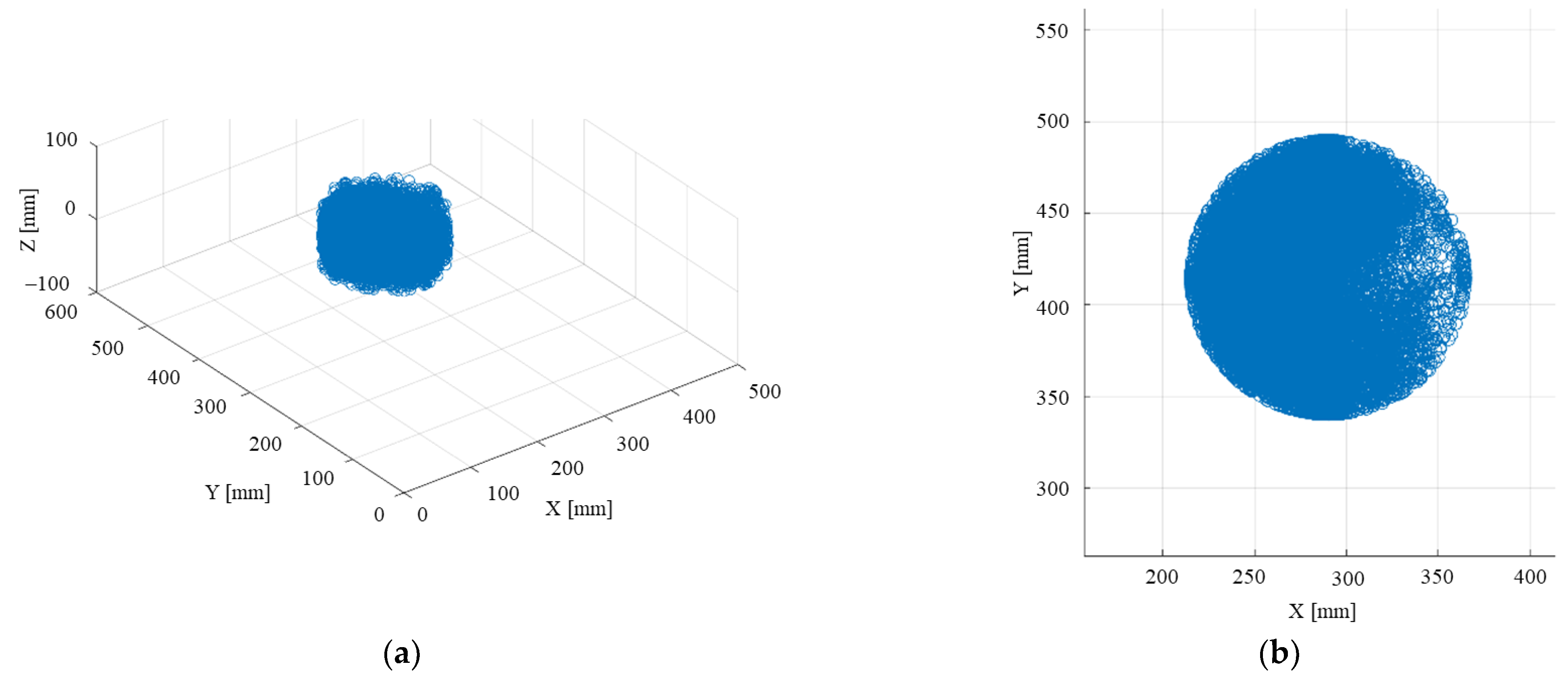
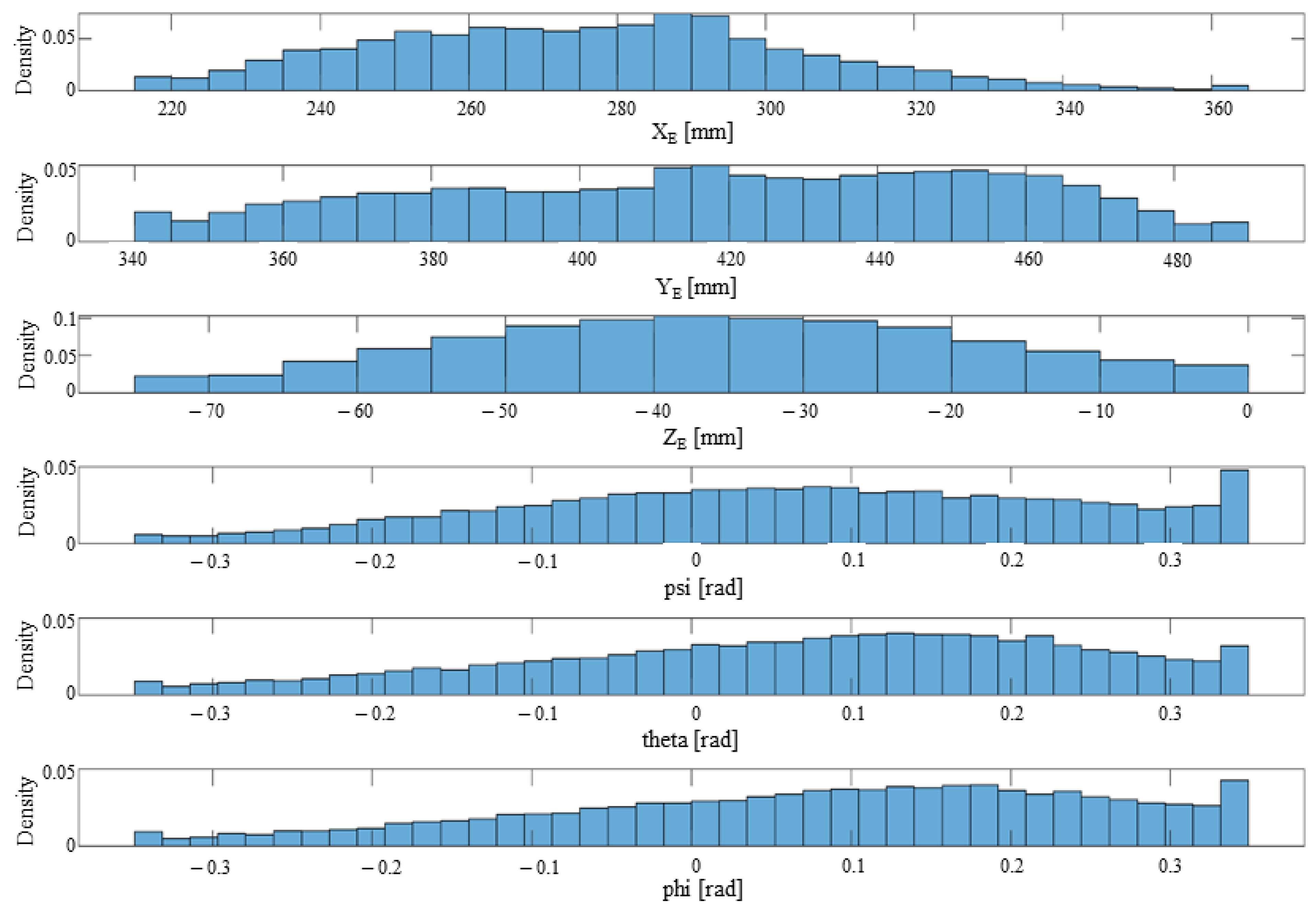
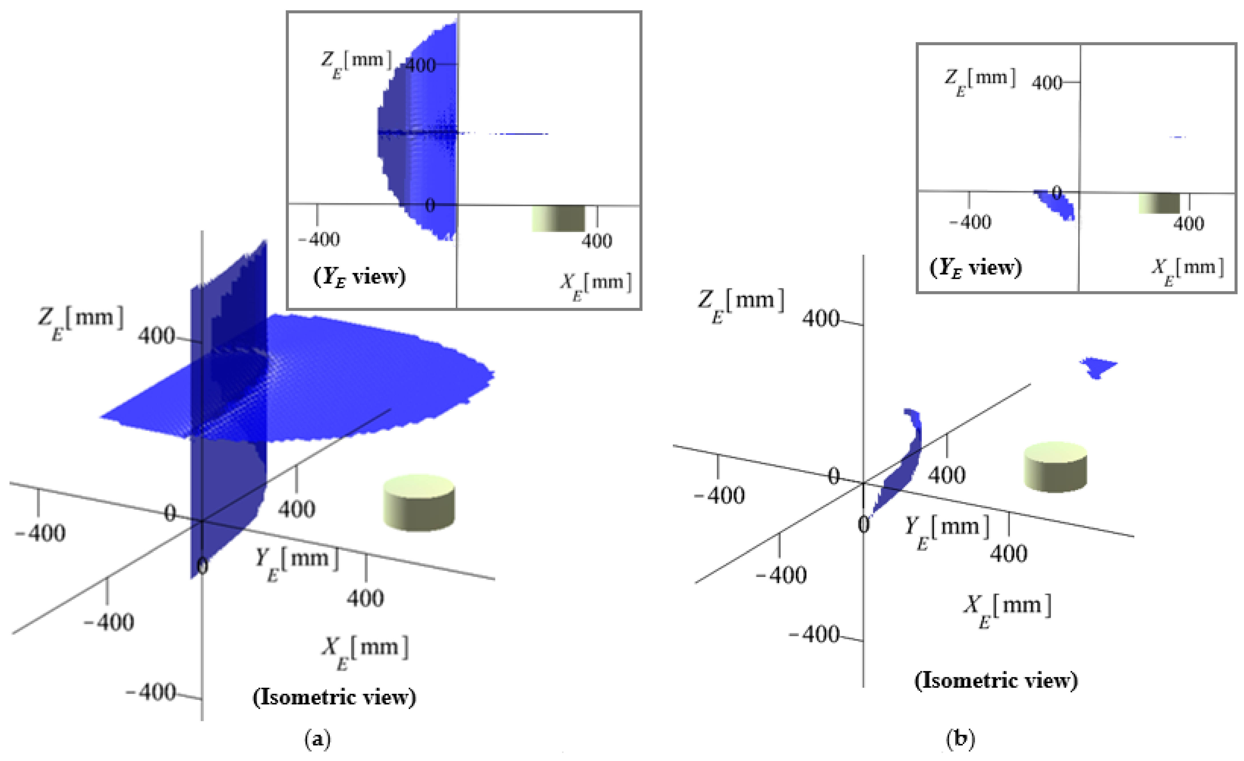
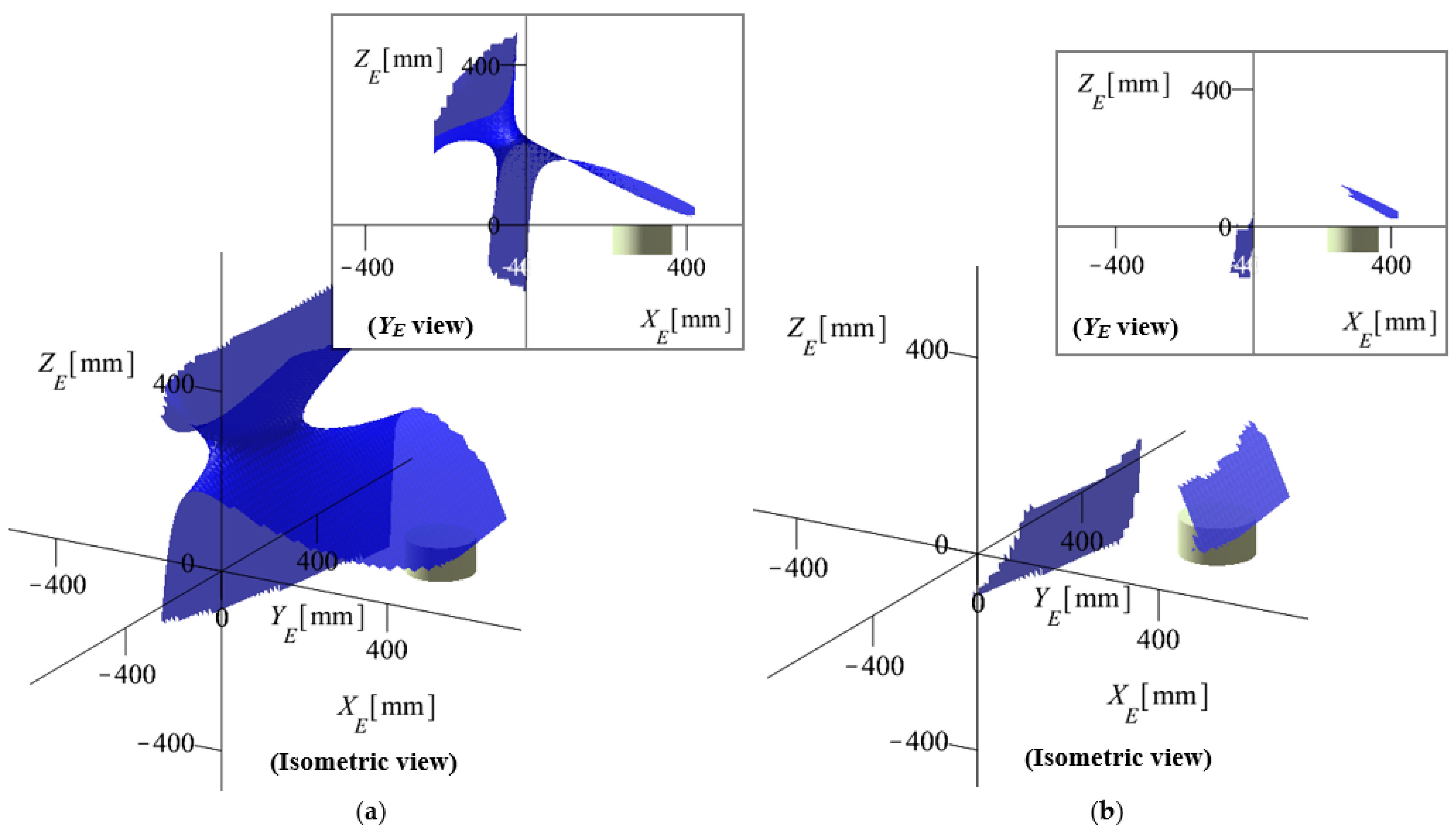
  • The gamultiobj function was iterated 200 times with the defined parameters, and with each iteration, the data were saved within the solution set SOLS. The gamultiobj function uses random number generators, and multiple iterations ensured that the optimized solution set spanned the “entire” operational workspace. The hypothesis is that the large number of solutions that spanned the entire operational workspace led to a better probability of finding feasible solutions (that are tested with the WS_DATA) in the next step. The set SOLS(m) (m = 1,…,28,568) includes numerical values for the mobile platform coordinates, the geometric parameters, and the active joints. Figure 15 illustrates a point cloud based on the Cartesian coordinates within SOLS(m) (m = 1,…,28,568), whereas Figure 16 illustrates the distribution of SOLS(m) (m = 1,…,28,568) with respect to the mobile platform coordinates.
  • A subset SOL(k) (k = 1, …, 931) was selected from SOLS(m) (m = 1, …, 28,568) which yield real values for qi (i = 1, …, 6) for all mobile platform coordinates in WS_DATA. Furthermore, the ranges Q_RANGE(k) for qi (i = 1, …, 6) of each solution the subset SOL(k) were evaluated to determine which solutions yield feasible mechanisms (where, e.g., the actuation axes do not cross). For the viable solutions FINAL(h) (h = 1, …, 9), the GCI was computed for the WS_DATA. Table 1 shows the resulting feasible solutions (FINAL(h)) for the geometric parameters of the 6-DOF parallel robot for SILS.
  • The design solution was Sol. no. 1 from Table 1, not because it has the best value for GCIa, but because it shows a “good” compromise between the footprint (e.g., LH) and the computed GCIa index (it ranks third with respect to LH and first with respect to GCIa). Table 2 shows the ranges of the active joins for the selected design solution.
Other authors used the NSGA-II algorithm [37] for multi-objective optimization problems (see, e.g., [38]) due to its computational efficiency and algorithm stability. Furthermore, there is no guarantee that the optimization algorithm used in this work yields a global optimum solution. However, based on multiple runs of the optimization algorithm (which yielded very similar results), the conclusion that the resulting design solutions are at least stable local ones is not implausible.

6.2. The Optimized Model of the 6-DOF Parallel Robot

Figure 17 shows the CAD model of the design solution of the 6-DOF parallel robot for SILS. Figure 17a shows the proposed relative position between the robotic system and the patient. Figure 17b shows the CAD model of the 6-DOF parallel robot with its actuators. The actuator positions are an initial concept that are subject to change in the later design stages based on the technical requirements and constraints.

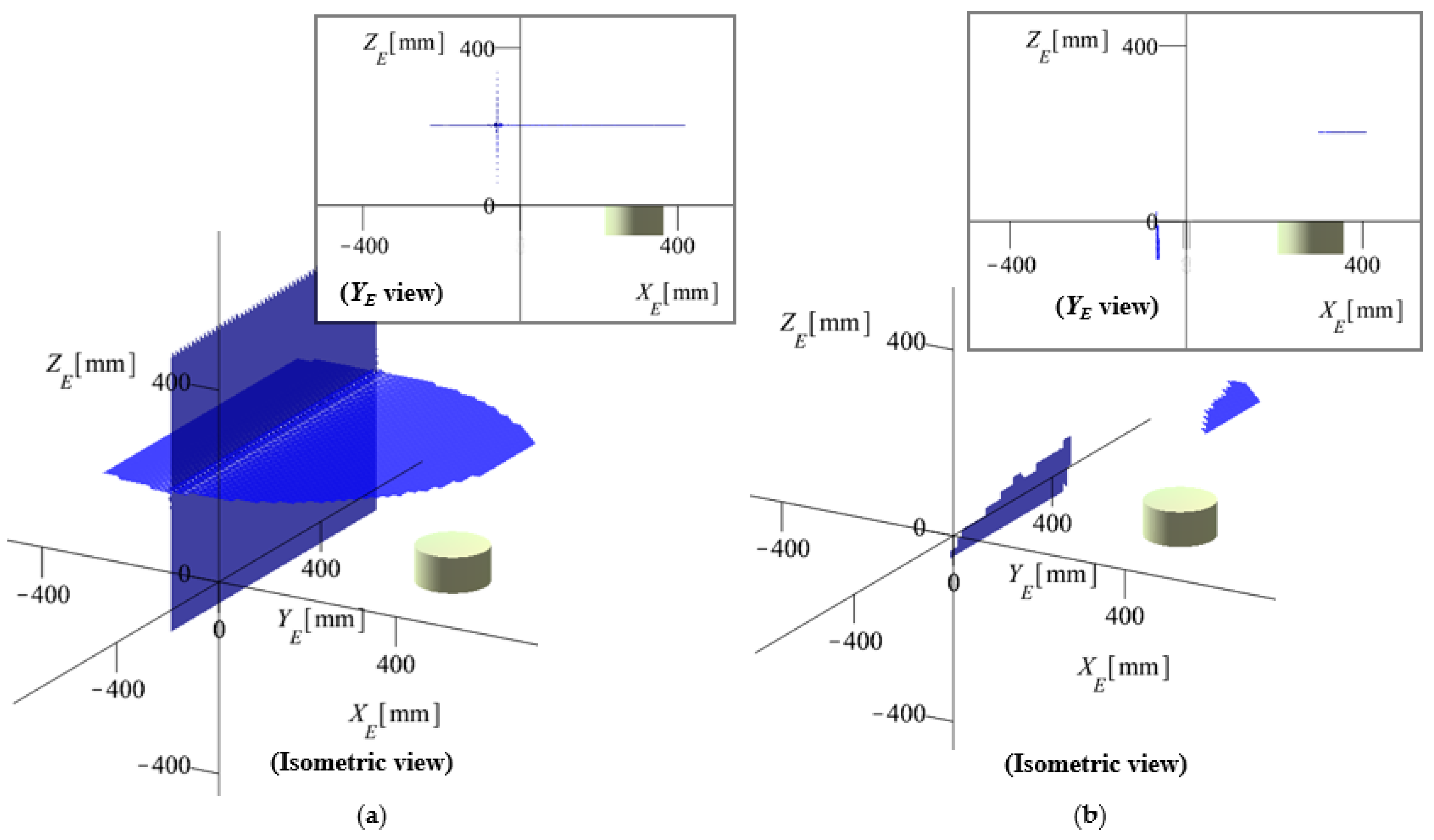
6.3. The Singularities of the Optimized Model of the 6-DOF Parallel Robot

The output singularities for the optimized model were studied by slicing the 6-dimensional (singular) configuration hyperspace, i.e., the numerical values for the angles ψ, θ, and φ were substituted into the singularity factor F (Equation (A1)—Appendix A), and the implicit surfaces (for XE, YE, and ZE) were plotted in Cartesian space.
Figure 18a illustrates the implicit surfaces for the given values of angles ψ, θ, and φ within the interval [–20, 20] [°] using an increment of 2°. Note that not all orientations defined by ψ, θ, and φ were associated with a color, but rather only the ψ angle was used in the surface color definition to avoid using a large number for surface colors (9261 colors were needed if each surface was assigned with a color). One important note is that no singularity surface intersects the operational workspace cylinder. Furthermore, these surfaces describe the output singularities without considering the inverse kinematic model. A second computation was made by considering the inverse kinematic model, i.e., the points on the surface were checked to yield real solutions for {q1, q2, q3, q4, q5, q6}, and are also within the intervals defined in Table 2. Figure 18b illustrates the results of this computation as implicit singularity surfaces. These surfaces show roughly where a singularity may occur for the 6-DOF parallel robot for SILS.
Some specific singularity surfaces (arbitrarily chosen) are presented next for better detail. Figure 19 shows the surface for the angle values {ψ = 0, θ = 0, φ = 0} [°], illustrating both the output singularity surface (Figure 19a) and the surface which degenerates after applying the inverse kinematic model constraints (Figure 19b). Figure 20 illustrates a possible singular configuration for the surface presented in Figure 19b (which is an output singularity of Case 5). Figure 21 and Figure 22 show the surfaces for the angle values {ψ = 20, θ = 0, φ = 0} [°] and {ψ = 20, θ = 20, φ = 20} [°], respectively.
Following the singularity analysis for the optimized model, a conjecture was proposed: Even though there exist output singularities in the robot workspace, there are none in the operational workspace. Based on this, the factor F (Equation (A1)—Appendix A) must be implemented in the robot control as an avoidance function to (i) avoid losing robot control in the positioning stage (when the robot positions the surgical instruments at the insertion points) and (ii) to avoid damaging the robot (e.g., in homing sequences or laboratory tests). Factor F can be implemented in the robot Programable Logic Controller (PLC) in the motion control functions and tested during the robot motion sequences, when (ideally) F becomes zero or (more often) changes its sign between two consecutive points if a singular pose is reached and the robot will stop. As these cases can appear only outside the operational workspace, when the instruments are not inserted in the body, the user can then move the robot using an alternative trajectory. When a Point to Point (PTP) algorithm is used, the entire trajectory can be checked before the actual robot motion and validated (using the F factor value as discussed before).

6.4. Numerical Simulations

The kinematic models of the 6-DOF parallel robot for SILS (the 3-R-PRR-PRS parallel robot) were derived in [27]. Considering the inverse kinematic models:
  Q ˙ = B 1 · A ·   X ˙   Q ¨ = B 1 ·   A ˙ ·   X ˙ + A ·   X ¨ +   B ˙ ·   Q ˙
With the Jacobian matrices, A and B, computed from Equation (7) and the inverse geometric model from Equation (5). An input trajectory was provided for the mobile platform coordinates and their velocity   Q ˙ and acceleration   Q ¨ vectors, respectively. The trajectory was defined as a sequence of motions in accordance with the medical protocol:
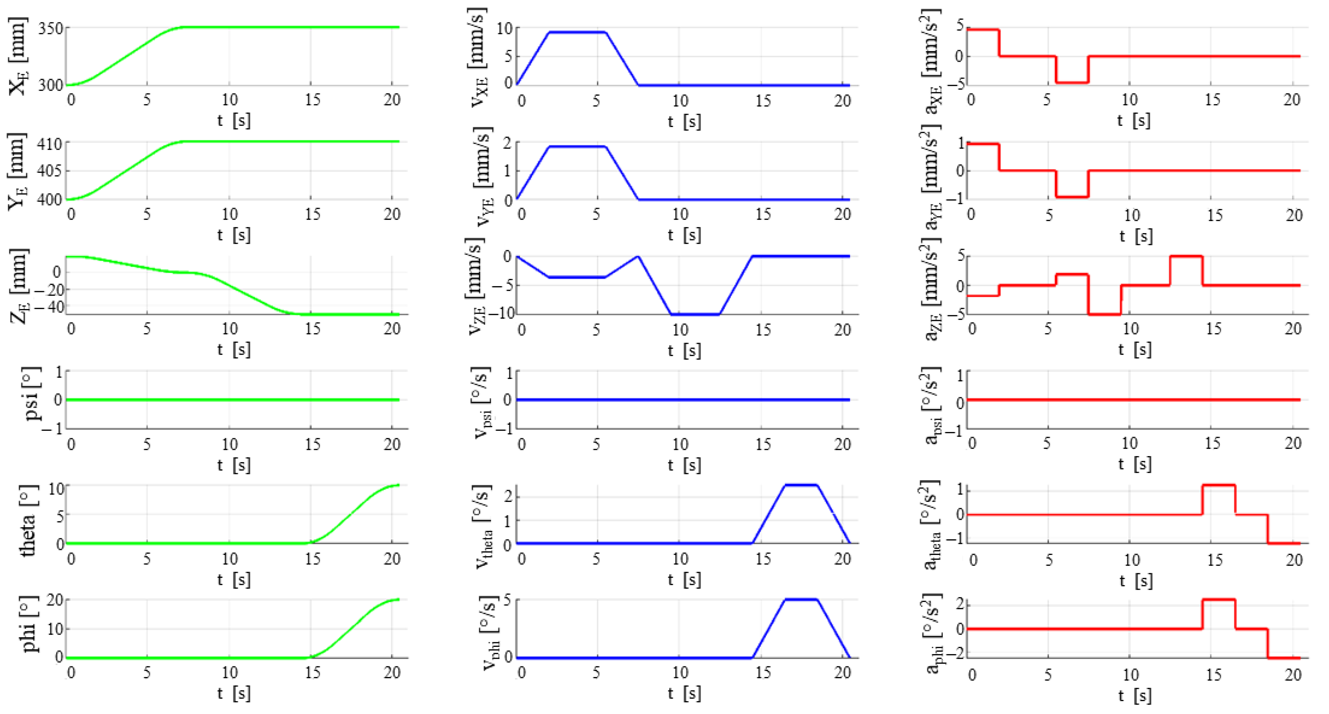
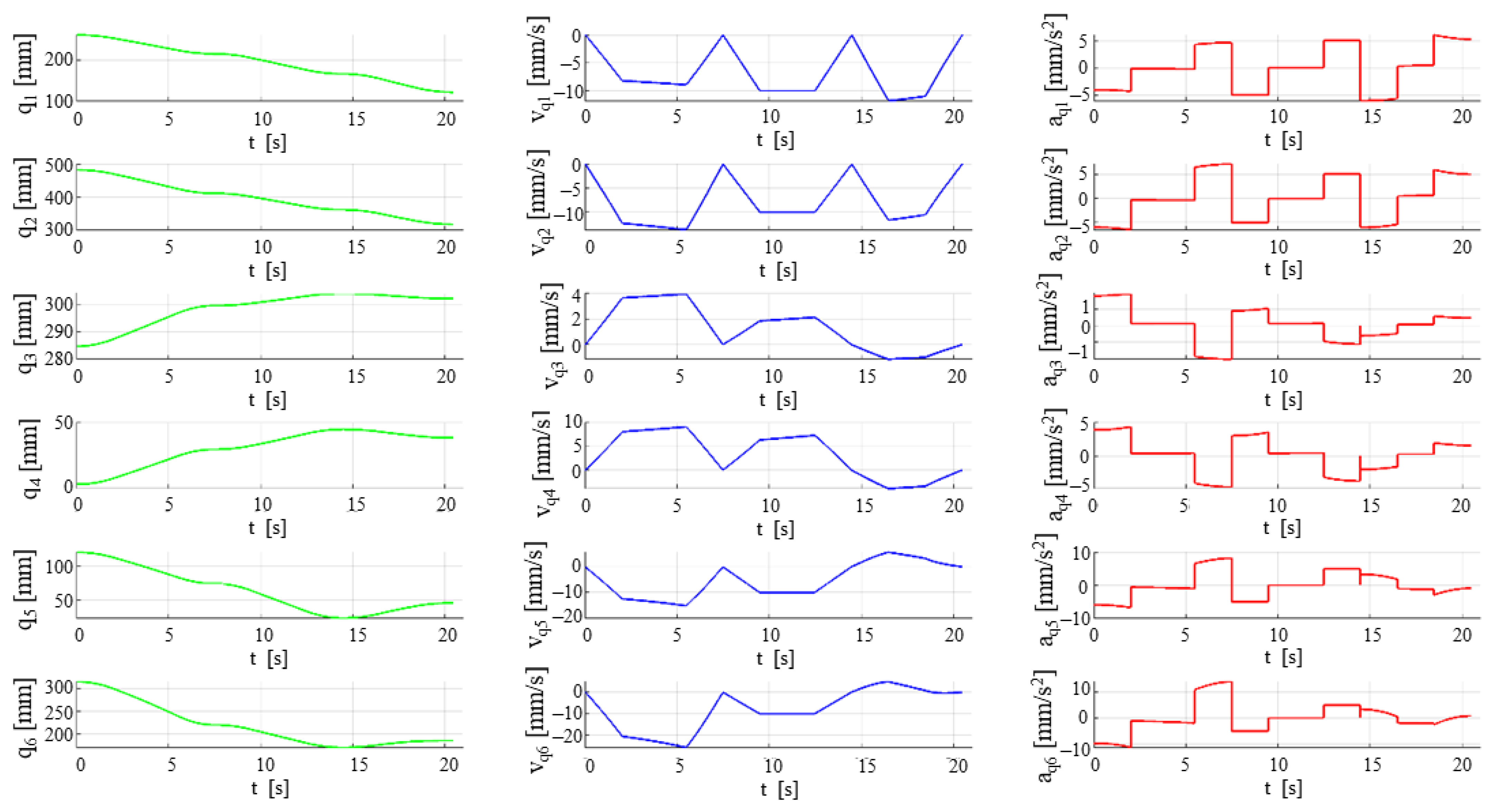
Stage 1 (align the medical instruments with the insertion points): linear motions from point E1 [X1 = 300, Y1 = 400, Z1 = 20, ψ1 = 0, θ1 = 0, ψ1 = 0] [mm, °] to point E2 [X2 = 350, Y2 = 410, Z2 = 0, ψ2 = 0, θ2 = 0, ψ2 = 0] [mm, °], with maximum velocity v_max = 10 mm/s and maximum acceleration a_max = 5 mm/s2;
Stage 2 (insert the instruments—the mobile platform positions the orientation platform RCM’s at the insertion points): linear motions from point E2 [X2 = 340, Y2 = 410, Z2 = 0, ψ2 = 0, θ2 = 0, ψ2 = 0] [mm, °] to point E3 [X3 = 350, Y3 = 410, Z3 = -50, ψ3 = 0, θ3 = 0, ψ3 = 0] [mm, °], with maximum velocity v_max = 10 mm/s and maximum acceleration a_max = 5 mm/s2;
Stage 3 (reorient the mobile platform): orientation motions from point E3 [X3 = 350, Y3 = 410, Z3 = −50, ψ3 = 0, θ3 = 0, ψ3 = 0] [mm, °] to point E4 [X4 = 350, Y4 = 410, Z4 = −50, ψ4 = 0, θ4 = 10, ψ4 = 20] [mm, °], with maximum v_max = 4 °/s and maximum acceleration a_max = 2 °/s2.
Figure 23 shows the time-dependent diagrams for the input trajectories, whereas Figure 24 shows the time-dependent diagrams for the active joints (computed via the inverse kinematic models). The results show no spikes and large (inadequate) values in the velocity and acceleration fields (which represents advantages in the further design stages when actuators must be chosen) and no violation of the active joint boundaries shown in Table 2.

7. Conclusions

This paper presented a singularity analysis using the vanishing points of the determinants of the Jacobian matrices and the geometric optimization of a 6-DOF parallel robot for SILS. Numerical analysis for the singularities, where slices of the 6-dimensional singularity hyperspace were studied for imposed orientation angles (correlated with the SILS task), showed that no singularity surface intersects the cylindrical operational workspace. The conjecture is that there are no singularities in the operational workspace (within the boundary of the maximum orientation values for the SILS task). However, the numerical analysis of the singularities also showed that there exist singularity configurations outside the operational workspace. Consequently, the singularity factor (of det(A)) must be implemented in the robotic system control to avoid these configurations. Numerical simulations based on the optimized parallel robot for SILS were performed to validate the proposed solution for the medical task.
Further work is intended for the next development stages of the robotic system, such as designing (prototyping and CAD design), simulating (motion simulations and finite element analysis), and testing the experimental model in laboratory medically-relevant conditions.

Author Contributions

Conceptualization, D.P. and I.B.; data curation, A.P., P.T., N.C., I.A., C.R. and B.G.; formal analysis, D.P., B.G. and C.V.; funding acquisition, D.P.; investigation, I.B., A.P., P.T. and C.V.; methodology, I.B. and C.V.; supervision, D.P.; validation, D.P.; visualization, P.T.; writing—original draft, I.B., A.P. and C.V.; writing—review & editing, D.P., P.T. and B.G. All authors have read and agreed to the published version of the manuscript.

Funding

This work was supported by a grant of the Ministry of Research, Innovation and Digitization, CNCS/CCCDI—UEFISCDI, project number PCE171/2021—Challenge within PNCDI III, and project POCU/380/6/13/123927–ANTREDOC, “Entrepreneurial competencies and excellence research in doctoral and postdoctoral studies programs”, a project co-funded by the European Social Fund through the Human Capital Operational.

Institutional Review Board Statement

Not applicable.

Informed Consent Statement

Not applicable.

Data Availability Statement

Not applicable.

Conflicts of Interest

The authors declare no conflict of interest.

Appendix A

F = 24 X E 3 c ψ 2 c φ 2 s θ + 12 X E Y E 2 c ψ 2 s θ + 12 X E Y E 2 c φ 2 s θ 12 L H X E 2 c φ s φ + 24 X E 2 Y E c φ s φ 12 X E 3 c ψ 2 s θ 12 X E 3 c φ 2 s θ + 12 X E 3 s θ + 24 X E 3 c φ s φ c ψ s ψ 12 X E 2 Y E c θ 2 c φ s φ 12 L H X E Y E c ψ 2 s θ + 12 L H X E 2 c ψ s ψ s θ 12 L H X E Y E c φ 2 s θ 24 X E 2 Y E c ψ s ψ s θ + 2 l p 2 L V c θ 3 c φ 2 c ψ 2 l p 2 Z E c θ 3 c φ 2 c ψ 24 X E Y E 2 c ψ 2 c φ 2 s θ + 3 l p L H L V c φ 3 c θ + 24 L H X E 2 c ψ 2 c φ s φ 3 l p L H Z E c φ 3 c θ + 6 L H X E 2 c θ 2 c φ s φ 12 L V X E 2 c φ 2 c ψ c θ 48 X E 2 Y E c ψ 2 c θ s θ + 12 X E 2 Z E c φ 2 c ψ c θ + 4 3 l p L H Y E c θ 3 c ψ 2 s ψ c φ + 2 3 l p L H L V c ψ 2 c θ 2 s θ s φ + 8 3 l p L H X E c ψ 2 c φ 2 s ψ c θ s θ 2 3 l p L H Z E c ψ 2 c θ 2 s θ c φ s φ 4 3 l p L V Y E c ψ 2 c θ 2 s θ c φ s φ 4 3 l p X E 2 c ψ c θ s θ 3 l p 2 L H c φ 3 c θ s θ + 4 3 l p X E 2 c ψ 3 c θ s θ 4 3 l p Y E 2 c ψ 3 c θ s θ 2 3 l p L V X E c φ 2 c θ 2 + 2 3 X E Z E c φ 2 c θ 2 + 6 3 L H X E 2 c φ c θ s θ 3 l p L H X E c φ 2 s ψ c θ s θ + 8 3 l p X E Y E c ψ 2 s ψ c θ s θ + 2 3 l p X E Y E c φ 2 s ψ c θ s θ + 5 3 l p L H X E c ψ c θ c φ s φ + 2 3 l p 2 L H c φ 2 s φ c ψ s ψ c θ 2 3 l p L H X E c θ 3 c ψ c φ s φ + 4 3 l p L V Y E c φ 2 c θ 2 c ψ s ψ + 16 3 l p X E Y E c ψ 3 c θ c φ s φ 8 3 l p X E 2 c ψ 2 c θ s θ c φ s ψ + 8 3 l p Y E 2 c ψ 2 c θ s θ c φ s ψ 4 3 l p X E Z E c φ 2 c θ 2 c ψ s ψ + 4 3 l p X E Y E c θ 3 c ψ c φ s φ 4 3 l p L H X E c ψ 2 s ψ c θ s θ 10 3 l p X E Y E c ψ c θ c φ s φ + 4 3 l p L H X E c ψ 3 c θ 3 c φ s φ 3 l p 2 L H c θ 3 c φ 2 s φ c ψ s ψ 4 3 l p Y E 2 c θ 3 c ψ 2 s ψ c φ s φ 8 3 l p L H Y E c ψ 3 c φ 2 c θ s θ 2 3 l p L H L V c φ 2 c θ 2 c ψ s ψ 8 3 l p L H X E c ψ 3 c θ c φ s φ + 2 3 l p L H Z E c φ 2 c θ 2 c ψ s ψ + 4 3 l p L H Y E c φ 2 c ψ c θ s θ + 4 3 l p L V X E c θ 2 s θ c φ s φ c ψ s ψ 4 3 l p X E Z E c θ 2 s θ c φ s φ c ψ s ψ + 4 3 l p L V X E c ψ 2 c φ 2 c θ 2 4 3 l p X E Z E c ψ 2 c φ 2 c θ 2 + 4 3 l p L H Y E c ψ 3 c θ s θ 3 l p 2 L H c ψ 2 c φ c θ s θ + 6 3 l p X E 2 c φ 2 c ψ c θ s θ 4 3 l p Y E 2 c φ 2 c ψ c θ s θ 6 3 L H L V X E c θ 2 c ψ c φ + 6 3 L H X E Z E c θ 2 c ψ c φ + 2 3 l p X E 2 c ψ c θ c φ s φ + 2 3 l p 2 L H c φ 3 c ψ 2 c θ s θ 8 3 l p X E 2 c ψ 3 c φ 2 c θ s θ + 8 3 l p Y E 2 c ψ 3 c φ 2 c θ s θ 16 3 l p X E Y E c ψ 2 c φ 2 s ψ c θ s θ + 4 3 l p Y E Z E c ψ 2 c θ 2 c φ s φ s θ 8 3 l p L H Y E c ψ 2 s ψ c φ c θ s θ 6 l p L H L V c φ 2 s φ c ψ s ψ c θ s θ + 6 l p L H Z E c φ 2 s φ c ψ s ψ c θ s θ + 3 l p L H L V c φ 3 c θ 3 c ψ 2 3 l p L H Z E c φ 3 c θ 3 c ψ 2 2 l p 2 X E c φ 2 c θ 2 c ψ 2 s θ 6 l p L H L V c φ 3 c ψ 2 c θ 6 l p L H L V c θ 3 c ψ 2 c φ + 6 l p L H Z E c φ 3 c ψ 2 c θ + 6 l p L H Z E c θ 3 c ψ 2 c φ 12 L H X E 2 c ψ 2 c θ 2 c φ s φ l p 2 L H c ψ 2 c θ 2 c φ s φ + 24 X E 2 Y E c ψ 2 c θ 2 c φ s φ + 2 l p 2 Y E c ψ 2 c θ 2 c φ s φ 12 X E 3 c θ 2 c ψ s ψ c φ s φ + 24 L H X E Y E c ψ 2 c φ 2 s θ 24 L H X E 2 c φ 2 s θ c ψ s ψ + 48 X E 2 Y E c φ 2 s θ c ψ s ψ + 3 l p L H L V c ψ 2 c φ c θ + 6 L H L V X E c φ 2 s ψ c θ 3 l p L H Z E c ψ 2 c φ c θ 6 L H X E Z E c φ 2 s ψ c θ 12 L V X E Y E c φ 2 s ψ c θ 24 X E Y E 2 c ψ s ψ c θ s θ + 12 X E Y E Z E c φ 2 s ψ c θ 12 L V X E 2 s ψ c φ s φ c θ s θ + 12 X E 2 Z E s ψ c φ s φ c θ s θ + 24 L H X E Y E c ψ s ψ c φ s φ 3 l p L H X E c φ 3 c θ 2 s θ s ψ + l p 2 L H c φ 2 c θ 2 s θ c ψ s ψ 2 l p 2 Y E c φ 2 c θ 2 s θ c ψ s ψ 3 l p L H X E c θ 2 c φ 2 s φ s ψ + 12 X E Y E 2 c θ 2 c ψ s ψ c φ s φ 2 l p 2 X E c θ 2 c ψ s ψ c φ s φ + 6 l p L H X E c θ 2 s θ c ψ c φ 12 L H X E Y E c θ 2 c ψ s ψ c φ s φ 6 L H L V X E c θ s θ c φ s φ c ψ + 6 L H X E Z E c θ s θ c φ s φ c ψ + 12 L V X E Y E c θ s θ c φ s φ c ψ 12 X E Y E Z E c θ s θ c φ s φ c ψ

References

  1. Saidy, M.N.; Tessier, M.; Tessier, D. Single-Incision Laparoscopic Surgery—Hype or Reality: A Historical Control Study. Perm. J. 2012, 16, 47–50. [Google Scholar] [CrossRef] [PubMed]
  2. Ghezzi, T.L.; Corleta, O.C. 30 Years of Robotic Surgery. World J. Surg. 2016, 40, 2550–2557. [Google Scholar] [CrossRef] [PubMed]
  3. Pisla, D.; Andras, I.; Vaida, C.; Crisan, N.; Ulinici, I.; Birlescu, I.; Plitea, N. New approach to hybrid robotic system application in Single Incision Laparoscopic Surgery. Acta Teh. Napoc. 2021, 64, 369–378. [Google Scholar]
  4. Peters, B.S.; Armijo, P.R.; Krause, C.; Choudhury, S.A.; Oleynikov, D. Review of emerging surgical robotic technology. Surg. Endosc. 2018, 32, 1636–1655. [Google Scholar] [CrossRef] [PubMed]
  5. Kuo, C.-H.; Dai, J.S. Robotics for Minimally Invasive Surgery: A Historical Review from the Perspective of Kinematics. In International Symposium on History of Machines and Mechanisms; Yan, H.S., Ceccarelli, M., Eds.; Springer: Dordrecht, The Netherlands, 2009; pp. 337–354. [Google Scholar]
  6. Horgan, S.; Vanuno, D. Robots in laparoscopic surgery. J. Laparoendosc. Adv. Surg. Tech. 2001, 11, 415–419. [Google Scholar] [CrossRef]
  7. Beatrice, A.; Matthew, J.C.; Danail, S. Gesture Recognition in Robotic Surgery: A Review. IEEE Trans. Biomed. Eng. 2021, 68, 2021–2035. [Google Scholar]
  8. Saeidi, H.; Opfermann, J.D.; Kam, M.; Raghunathan, S.; Leonard, S.; Krieger, A. A Confidence-Based Shared Control Strategy for the Smart Tissue Autonomous Robot (STAR). In Proceedings of the 2018 IEEE/RSJ International Conference on Intelligent Robots and Systems (IROS), Madrid, Spain, 1–5 October 2018; pp. 1268–1275. [Google Scholar]
  9. Bhandari, M.; Zeffiro, T.; Reddiboina, M. Artificial intelligence and robotic surgery. Curr. Opin. Urol. 2020, 30, 48–54. [Google Scholar] [CrossRef]
  10. Harky, A.; Chaplin, G.; Chan, J.S.K.; Eriksen, P.; MacCarthy-Ofosu, B.; Theologou, T.; Muir, A.D. The Future of Open Heart Surgery in the Era of Robotic and Minimal Surgical Interventions. Hear. Lung Circ. 2019, 29, 49–61. [Google Scholar] [CrossRef]
  11. Wang, W.; Sun, X.; Wei, F. Laparoscopic surgery and robotic surgery for single-incision cholecystectomy: An updated systematic review. Updat. Surg. 2021, 73, 2039–2046. [Google Scholar] [CrossRef]
  12. Kwak, Y.H.; Lee, H.; Seon, K.; Lee, Y.J.; Lee, Y.J.; Kim, S.W. Da Vinci SP Single-Port Robotic Surgery in Gynecologic Tumors: Single Surgeon’s Initial Experience with 100 Cases. Yonsei Med. J. 2022, 63, 179–186. [Google Scholar] [CrossRef]
  13. McCarus, S.D. Senhance Robotic Platform System for Gynecological Surgery. JSLS J. Soc. Laparoendosc. Surg. 2021, 25, e2020.00075. [Google Scholar] [CrossRef]
  14. Laribi, M.A.; Mlika, A.; Romdhane, L.; Zeghloul, S. Robust Optimization of the RAF Parallel Robot for a Prescribed Workspace. In Computational Kinematics. Mechanisms and Machine Science; Zeghloul, S., Romdhane, L., Laribi, M., Eds.; Springer: Cham, Switzerland, 2018; Volume 50, pp. 383–393. [Google Scholar] [CrossRef]
  15. Hay, A.M.; Snyman, J.A. Optimal synthesis for a continuous prescribed dexterity interval of a 3-dof parallel planar manipulator for different prescribed output workspaces. Int. J. Numer. Methods Eng. 2006, 68, 1–12. [Google Scholar] [CrossRef]
  16. Merlet, J.P. Jacobian, manipulability, condition number, and accuracy of parallel robots. ASME J. Mech. Des. 2006, 128, 199–206. [Google Scholar] [CrossRef]
  17. Gosselin, C.; Angeles, J. A global performance index for the kinematic optimization of robotic manipulators. ASME. J. Mech. Des. 1991, 113, 220–226. [Google Scholar] [CrossRef]
  18. Itul, T.P.; Galdau, B.; Pisla, D.L. Static analysis and stiffness of a 2-dof parallel device for orientation. Acta Tech. Napoc. Ser. Appl. Math. Mech. Eng. 2012, 55, 615–620. [Google Scholar]
  19. Chablat, D.; Wenger, P. Architecture optimization of a 3-DOF translational parallel mechanism for machining applications, the orthoglide. IEEE Trans. Robot. Autom. 2003, 19, 403–410. [Google Scholar] [CrossRef]
  20. Dastjerdi, A.H.; Sheikhi, M.M.; Masouleh, M.T. A complete analytical solution for the dimensional synthesis of 3-DOF delta parallel robot for a prescribed workspace. Mech. Mach. Theory 2020, 153, 103991. [Google Scholar] [CrossRef]
  21. Courteille, E.; Deblaise, D.; Maurine, P. Design optimization of a Delta-like parallel robot through global stiffness performance evaluation. In Proceedings of the 2009 IEEE/RSJ International Conference on Intelligent Robots and Systems, St. Louis, MO, USA, 10–15 October 2009; pp. 5159–5166. [Google Scholar] [CrossRef]
  22. Wang, A.U.; Rong, W.B.; Qi, L.M.; Qin, Z.G. Optimal design of a 6-DOF parallel robot for precise manipulation. In Proceedings of the 2009 International Conference on Mechatronics and Automation, Changchun, China, 9–12 August 2009. [Google Scholar]
  23. Qiang, H.; Wang, L.; Ding, J.; Zhang, L. Multiobjective Optimization of 6-DOF parallel manipulator for desired total orientation workspace. Math. Probl. Eng. 2019, 2019, 5353825. [Google Scholar] [CrossRef]
  24. Aboulissane, B.; Haiek, D.E.; Bakkali, L.E.; Bahaoui, J.E. On the workspace optimization of parallel robots based on CAD approach. Procedia Manuf. 2019, 32, 1085–1092. [Google Scholar] [CrossRef]
  25. Surbhil, G.; Sankho, T.S.; Amod, K. Design optimization of minimally invasive surgical robot. Appl. Soft Comput. 2015, 32, 241–249. [Google Scholar]
  26. Lessard, S.; Bigras, P.; Bonev, I.A. A New Medical Parallel Robot and Its Static Balancing Optimization. J. Med. Devices 2007, 1, 272–278. [Google Scholar] [CrossRef]
  27. Pisla, D.; Pusca, A.; Tucan, P.; Gherman, B.; Vaida, C. Kinematics and workspace analysis of an innovative 6-dof parallel robot for SILS. Proc. Rom. Acad. Ser. A, 2022; in press. [Google Scholar]
  28. Pisla, D.; Carami, D.; Gherman, B.; Soleti, G.; Ulinici, I.; Vaida, C. A novel control architecture for robotic-assisted single incision laparoscopic surgery. Rom. J. Tech. Sciences. Appl. Mech. 2021, 66, 141–162. [Google Scholar]
  29. Birlescu, I.; Vaida, C.; Pusca, A.; Rus, G.; Pisla, D. A New Approach to Forward Kinematics for a SILS Robotic Orientation Platform Based on Perturbation Theory. In Advances in Robot Kinematics 2022; Altuzarra, O., Kecskeméthy, A., Eds.; Springer: Cham, Switzerland, 2022; Volume 24, pp. 171–178. [Google Scholar] [CrossRef]
  30. Ebert-Uphoff, I.; Lee, J.-K.; Lipkin, H. Characteristic tetrahedron of wrench singularities for parallel manipulators with three legs. Proc. Inst. Mech. Eng. Part C: J. Mech. Eng. Sci. 2002, 216, 81–93. [Google Scholar] [CrossRef]
  31. MathWorks. gamultiobj. Available online: https://ch.mathworks.com/help/gads/gamultiobj.html (accessed on 1 July 2022).
  32. Pisla, D.; Birlescu, I.; Vaida, C.; Tucan, P.; Gherman, B.; Plitea, N. Family of Modular Parallel Robots with Active Translational Joints for Single Incision Laparoscopic Surgery. OSIM A00733, 3 December 2021. [Google Scholar]
  33. Gosselin, C.; Angeles, J. Singularity analysis of closed-loop kinematic chains. IEEE Trans. Robot. Autom. 1990, 6, 281–290. [Google Scholar] [CrossRef]
  34. Zlatanov, D.; Fenton, R.G.; Benhabib, B. A Unifying Framework for Classification and Interpretation of Mechanism Singularities. J. Mech. Des. 1995, 117, 566–572. [Google Scholar] [CrossRef]
  35. Ma, O.; Angeles, J. Architecture singularities of platform manipulators. In Proceedings of the 1991 IEEE International Conference on Robotics and Automation, Sacramento, CA, USA, 9–11 April 1991; pp. 1542–1547. [Google Scholar]
  36. Spring, I.W. Euler parameters and the use of quaternion algebra in the manipulation of finite rotations. Mech. Mach. Theory 1986, 21, 365–373. [Google Scholar] [CrossRef]
  37. Deb, K.; Agrawal, S.; Pratap, A.; Meyarivan, T. A Fast Elitist Non-dominated Sorting Genetic Algorithm for Multi-objective Optimization: NSGA-II. In PPSN 2000: Parallel Problem Solving from Nature PPSN VI.; Lecture Notes in Computer Science; Springer: Berlin/Heidelberg, Germany, 2000; Volume 1917, pp. 849–858. [Google Scholar]
  38. Wang, W.; Wang, W.; Dong, W.; Yu, H.; Yan, Z.; Du, Z. Dimensional optimization of a minimally invasive surgical robot system based on NSGA-II algorithm. Adv. Mech. Eng. 2015, 7, 1687814014568541. [Google Scholar] [CrossRef]
Figure 1. The initial modules for the SILS robotic system: (a) the 6-DOF parallel robot; (b) mobile platform containing the laparoscope and two orientation platforms; (c) surgical instrument.
Machines 10 00764 g001
Figure 2. Kinematic scheme of the 6-DOF parallel robot for SILS.
Machines 10 00764 g002
Figure 3. The proposed intraoperative workspace for the SILS robotic system: (a) frontal plane view showing the desired workspace with respect to the ribcage; (b) transverse plane view of the desired workspace; (c) the workspace of the surgical instruments with respect to the insertion points (brown—laparoscope, blue and green—active instruments).
Machines 10 00764 g003
Figure 4. The proposed external workspace for the 6-DOF SILS robotic system (cylinder with radius 75 [mm] and height 75 [mm] and its position with respect to the ribcage).
Machines 10 00764 g004
Figure 5. Characteristic plane defined for the kinematic chain 1.
Machines 10 00764 g005
Figure 6. Characteristic tetrahedron for the 6-DOF parallel robot for SILS (nonsingular pose).
Machines 10 00764 g006
Figure 7. Type II singularity of the 6-DOF parallel robot for SILS (case 1—the characteristic tetrahedron faces and base intersect in a point): (a) parallel robot pose; (b) characteristic planes intersect in a point.
Machines 10 00764 g007
Figure 8. Type II singularity of the 6-DOF parallel robot for SILS (case 3—two faces of the characteristic tetrahedron and its base intersect in a line): (a) parallel robot pose; (b) characteristic planes intersect in a line.
Machines 10 00764 g008
Figure 9. Type II singularity of the 6-DOF parallel robot for SILS (Case 4—two faces of the characteristic tetrahedron are coplanar): (a) parallel robot pose; (b) characteristic planes.
Machines 10 00764 g009
Figure 10. Type II singularity of the 6-DOF parallel robot for SILS (case 5—one face and the base of the characteristic tetrahedron are coplanar): (a) parallel robot pose; (b) P2 and Pm are coplanar.
Machines 10 00764 g010
Figure 11. Type II singularity of the 6-DOF parallel robot for SILS (case 5—one face and the base of the characteristic tetrahedron are coplanar): (a) parallel robot pose; (b) P1 and Pm are coplanar.
Machines 10 00764 g011
Figure 12. Type II singularity of the 6-DOF parallel robot for SILS (case 7—one face and the base of the characteristic tetrahedron are coplanar and the other two faces of the tetrahedron are also coplanar): (a) parallel robot pose; (b) characteristic planes.
Machines 10 00764 g012
Figure 13. Type II singularity of the 6-DOF parallel robot for SILS (case 8—all the faces and the base of the characteristic tetrahedron are coplanar): (a) parallel robot pose; (b) characteristic planes.
Machines 10 00764 g013
Figure 14. The generated discrete workspace (WS_DATA) for the SILS robotic systems (only the Cartesian coordinates): (a) isometric view; (b) Z axis view.
Machines 10 00764 g014
Figure 15. Point cloud spanned by the solution set SOLS(m) (m = 1,…,28,568): (a) isometric view; (b) Z axis view.
Machines 10 00764 g015
Figure 16. Mobile platform coordinates distribution density for the solution set SOLS(m) (m = 1,…, 28,568).
Machines 10 00764 g016
Figure 17. CAD model of the optimized version of the parallel robotic system for SILS: (a) relative position between the robotic system and the patient; (b) the 6-DOF parallel robotic system for SILS.
Machines 10 00764 g017
Figure 18. Output singularity surfaces: (a) without the inverse kinematic model constraints; (b) with the inverse kinematic model constraints.
Machines 10 00764 g018
Figure 19. Output singularity surface for {ψ = 0, θ = 0, φ = 0} [°]: (a) without the inverse kinematic model constraints; (b) with the inverse kinematic model constraints.
Machines 10 00764 g019
Figure 20. Output singularity configuration for the angle values {ψ = 0, θ = 0, φ = 0}.
Machines 10 00764 g020
Figure 21. Output singularity surface for {ψ = 20, θ = 0, φ = 0} [°]: (a) without the inverse kinematic model constraints; (b) with the inverse kinematic model constraints.
Machines 10 00764 g021
Figure 22. Output singularity surface for {ψ = 20, θ = 20, φ = 20} [°]: (a) without the inverse kinematic model constraints; (b) with the inverse kinematic model constraints.
Machines 10 00764 g022
Figure 23. Time history diagrams of the input trajectory (position—green, velocity—blue, accelerations—red).
Machines 10 00764 g023
Figure 24. Time history diagrams of the active joints (position—green, velocity—blue, accelerations—red).
Machines 10 00764 g024
Table 1. Results from the geometric optimization algorithm.
Sol.
No.
lp
[mm]
LH
[mm]
LV
[mm]
l1
[mm]
l2
[mm]
l3
[mm]
l4
[mm]
GCIa
1215.25558.86237.03158.57596.12283.74342.680.192
2215.51599.99206.68156.04552.89269.82328.020.188
3211.56575.65237.92178.22480.05349.99326.120.175
4222.53580.55238.12173.55576.46283.69314.100.180
5232.36546.54228.56155.83536.28291.79328.110.157
6214.9506.28231.16155.45501.26282.31312.530.156
Table 2. Active joints ranges for the design solution.
q1 [mm]q2 [mm]q3 [mm]q4 [mm]q5 [mm]q6 [mm]
min38.2179.6197.86.8−60.880.4
max347.5592.1476.6398.8193.2465.2
Publisher’s Note: MDPI stays neutral with regard to jurisdictional claims in published maps and institutional affiliations.

