
An Oil Wear Particles Inline Optical Sensor Based on Motion Characteristics for Rotating Machines Condition Monitoring


Abstract
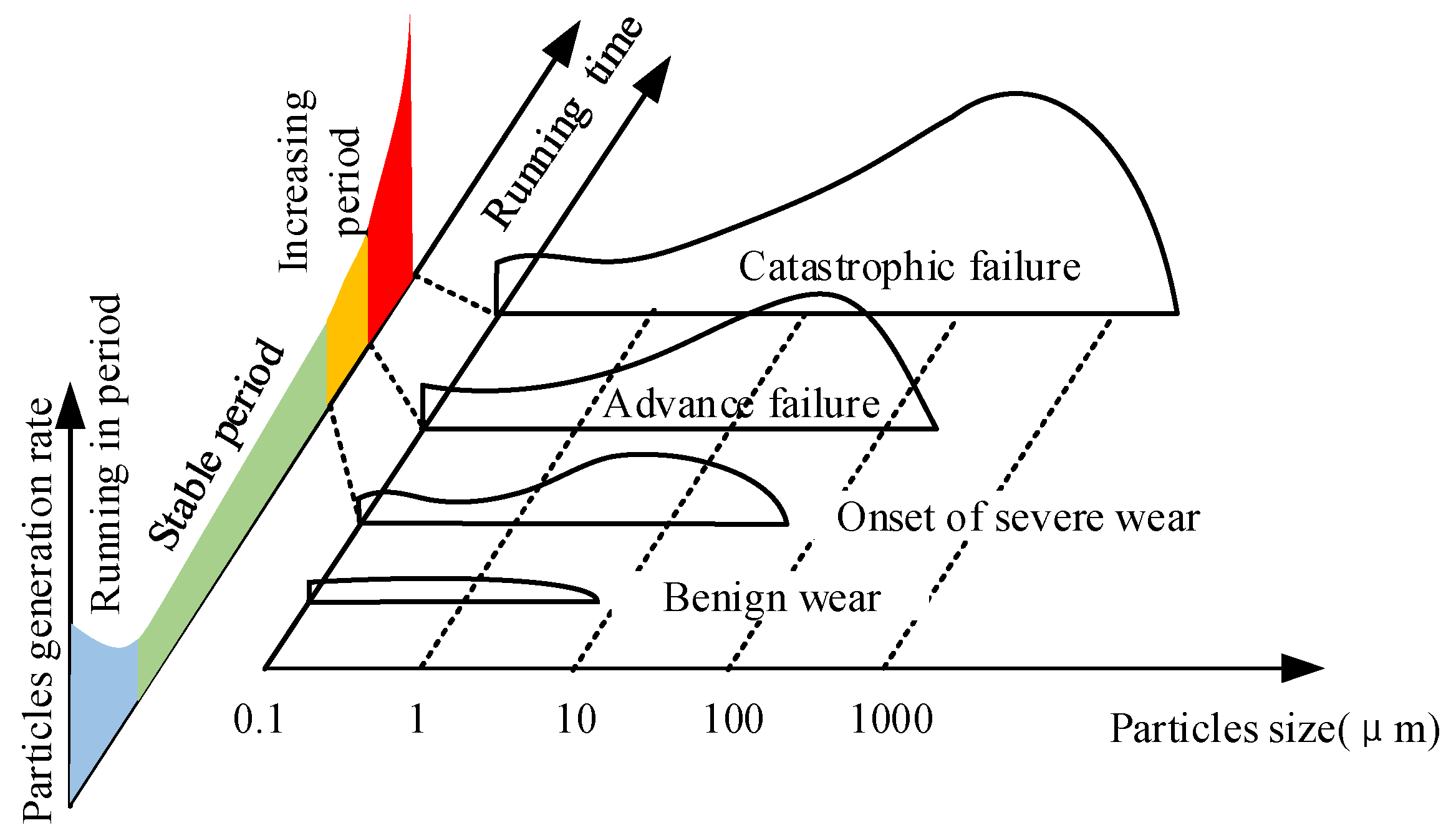
:1. Introduction
2. Materials and methods
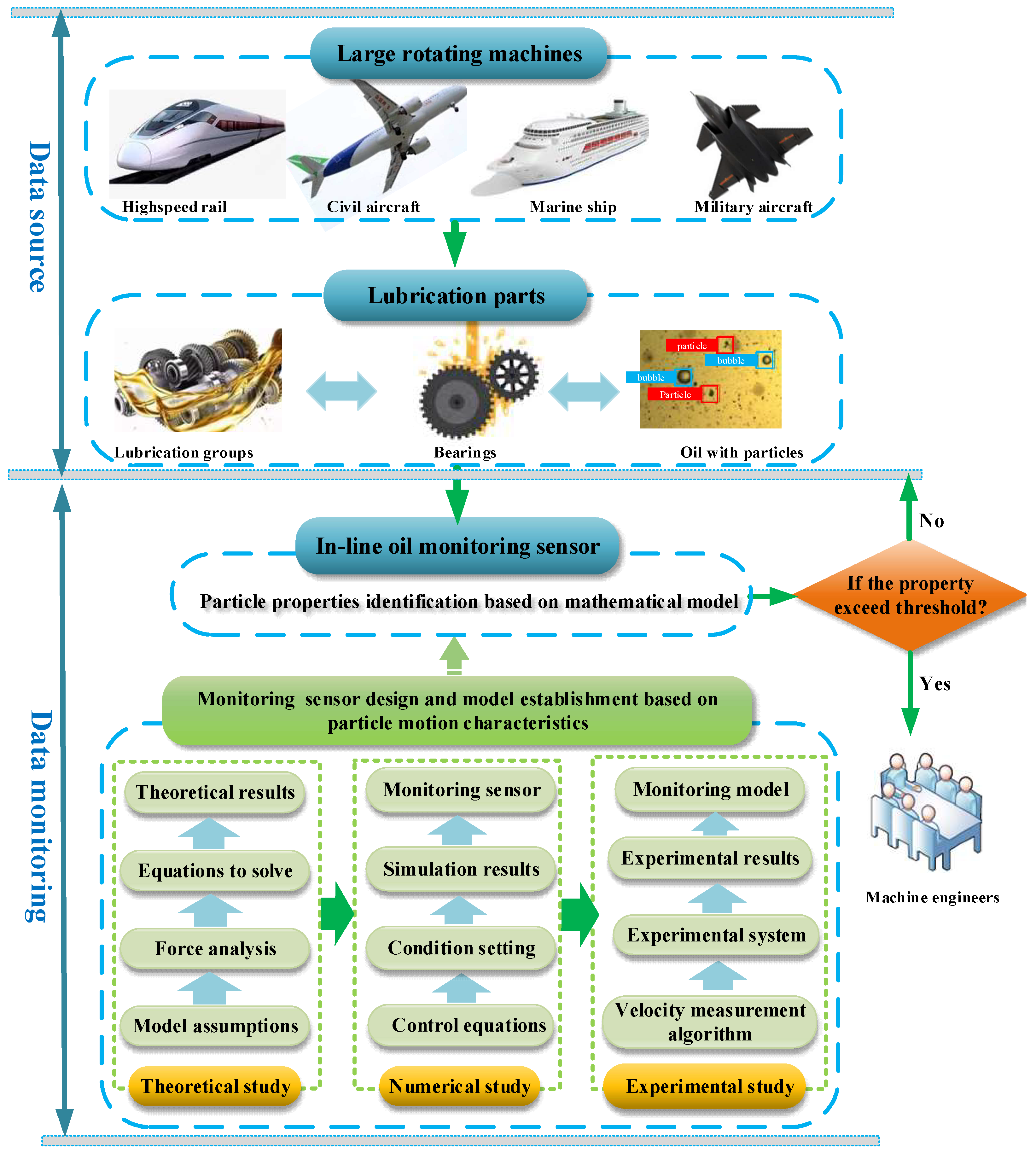
2.1. Framework
2.2. Methods of Analyzing Wear Particle Motion
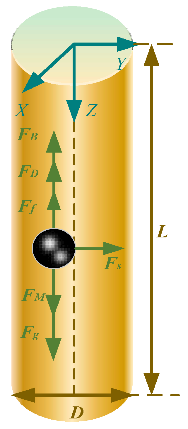
2.2.1. Theoretical Study
- (1)
- Oil was stationary.
- (2)
- Particles were rigid spherical particles.
- (3)
- Oil was an incompressible viscous fluid.
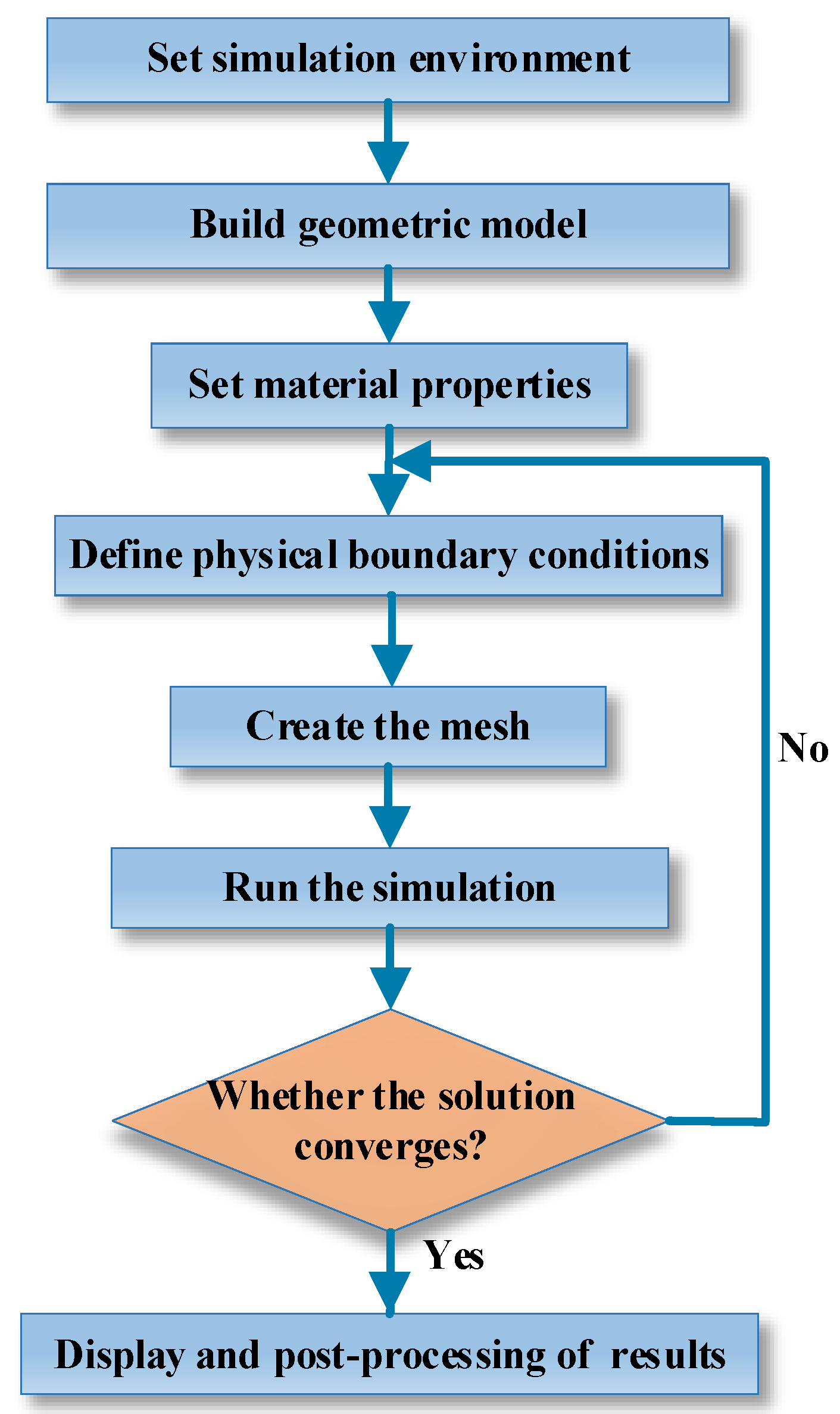
2.2.2. Numerical Study
3. Results and Discussion
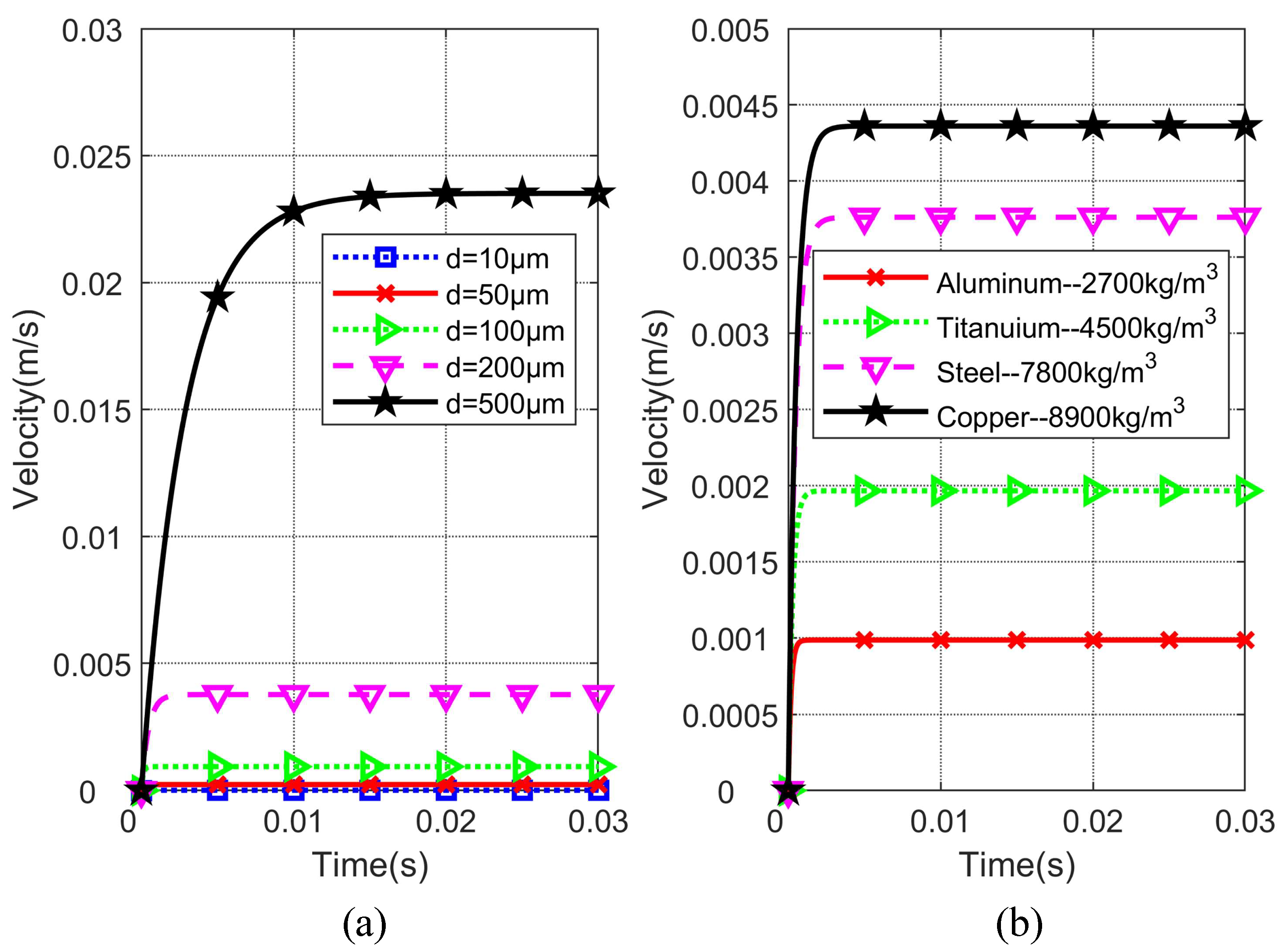
3.1. Theoretical Study Results
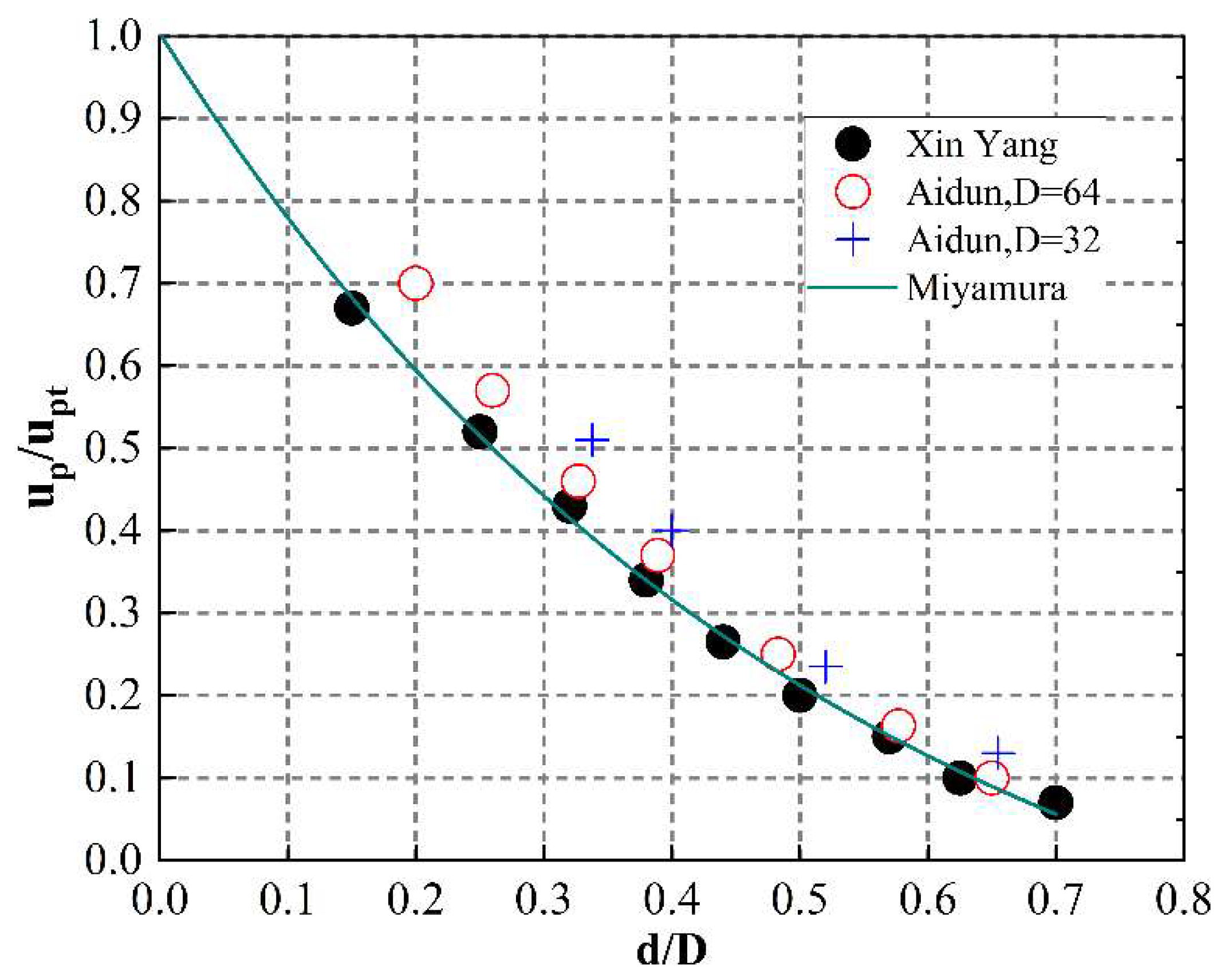
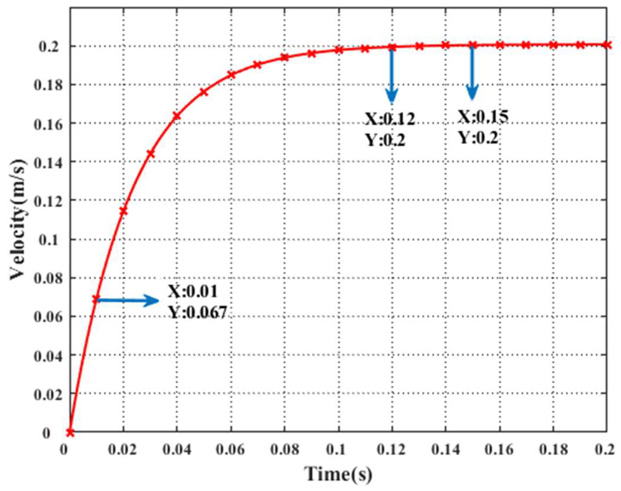
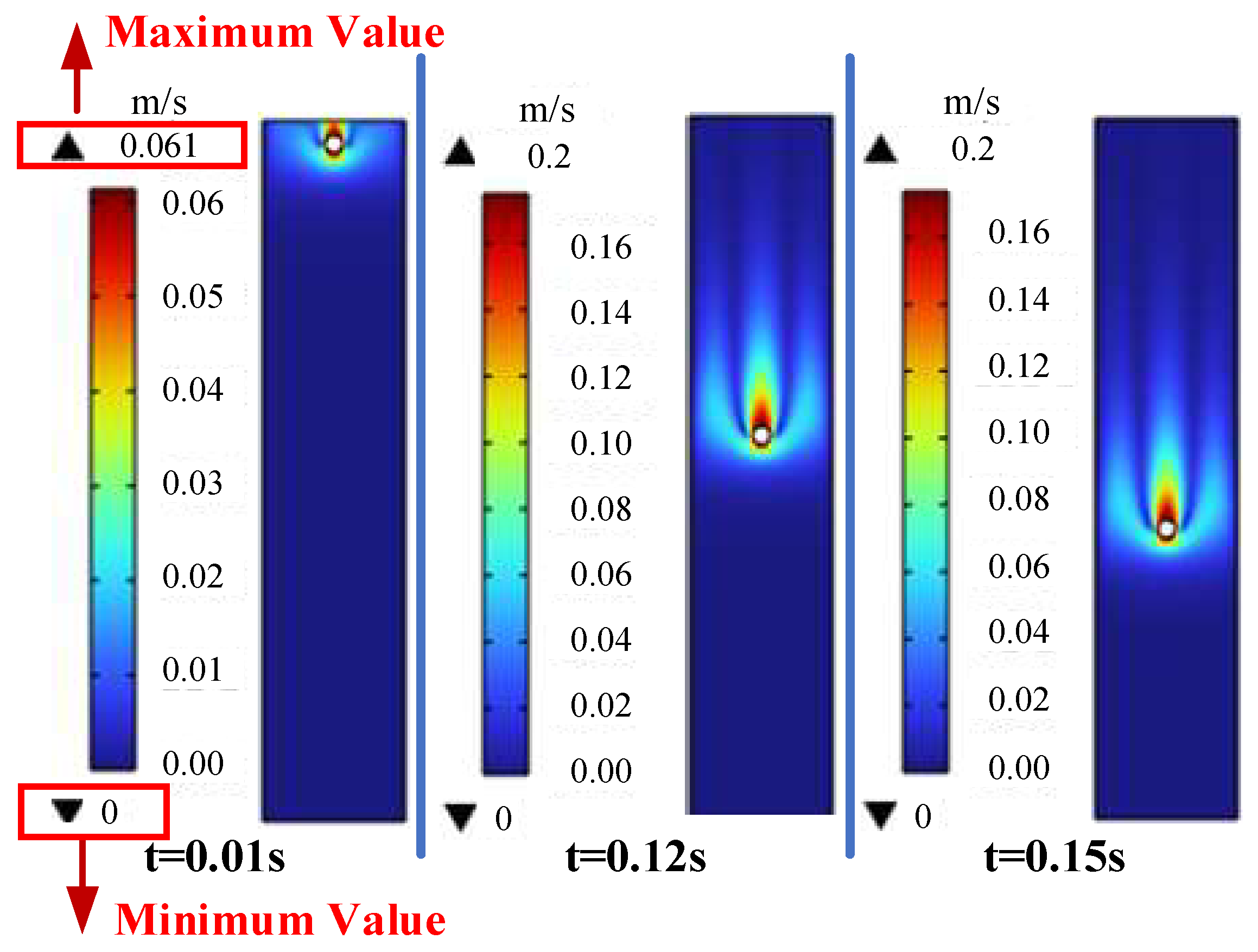
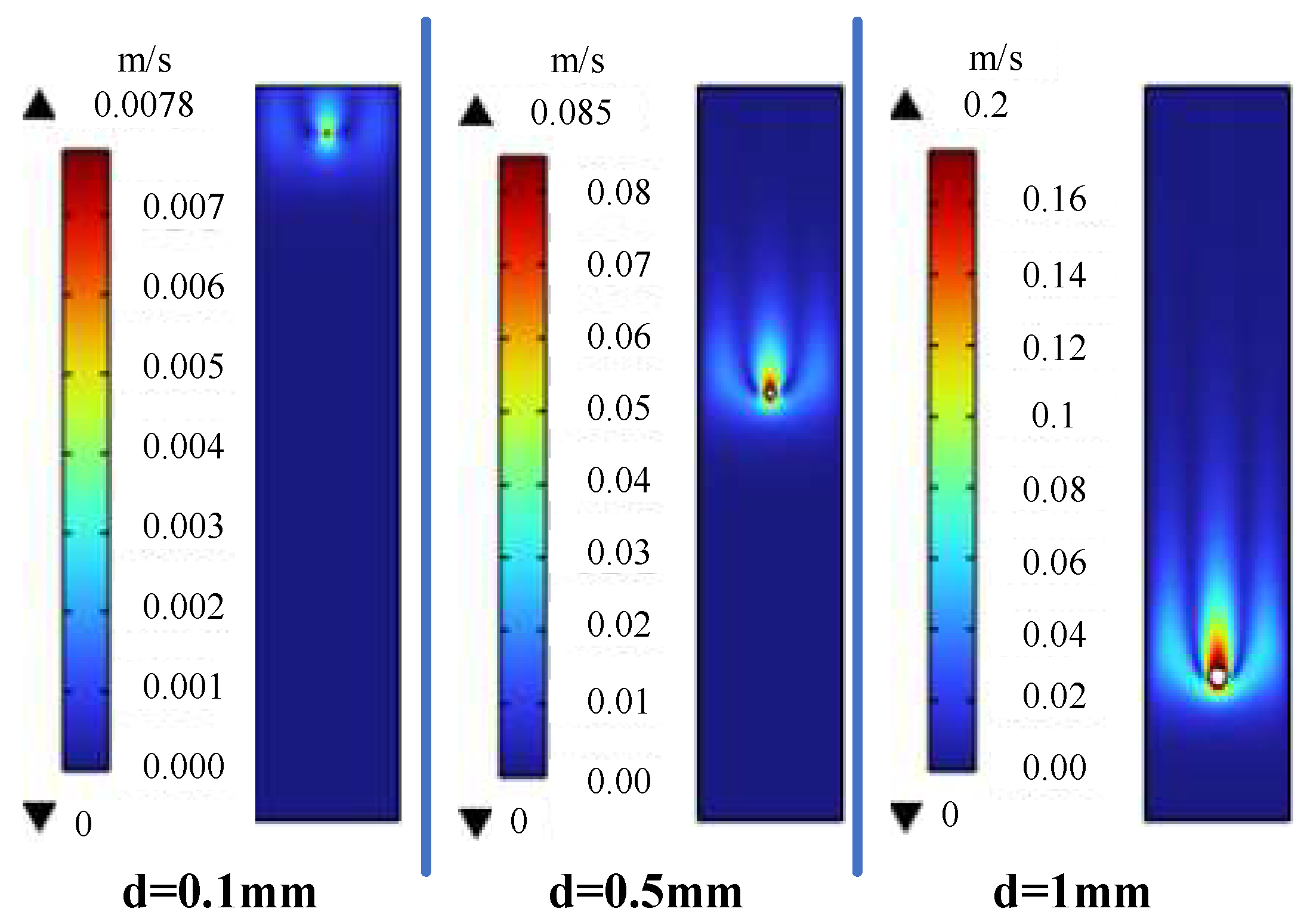
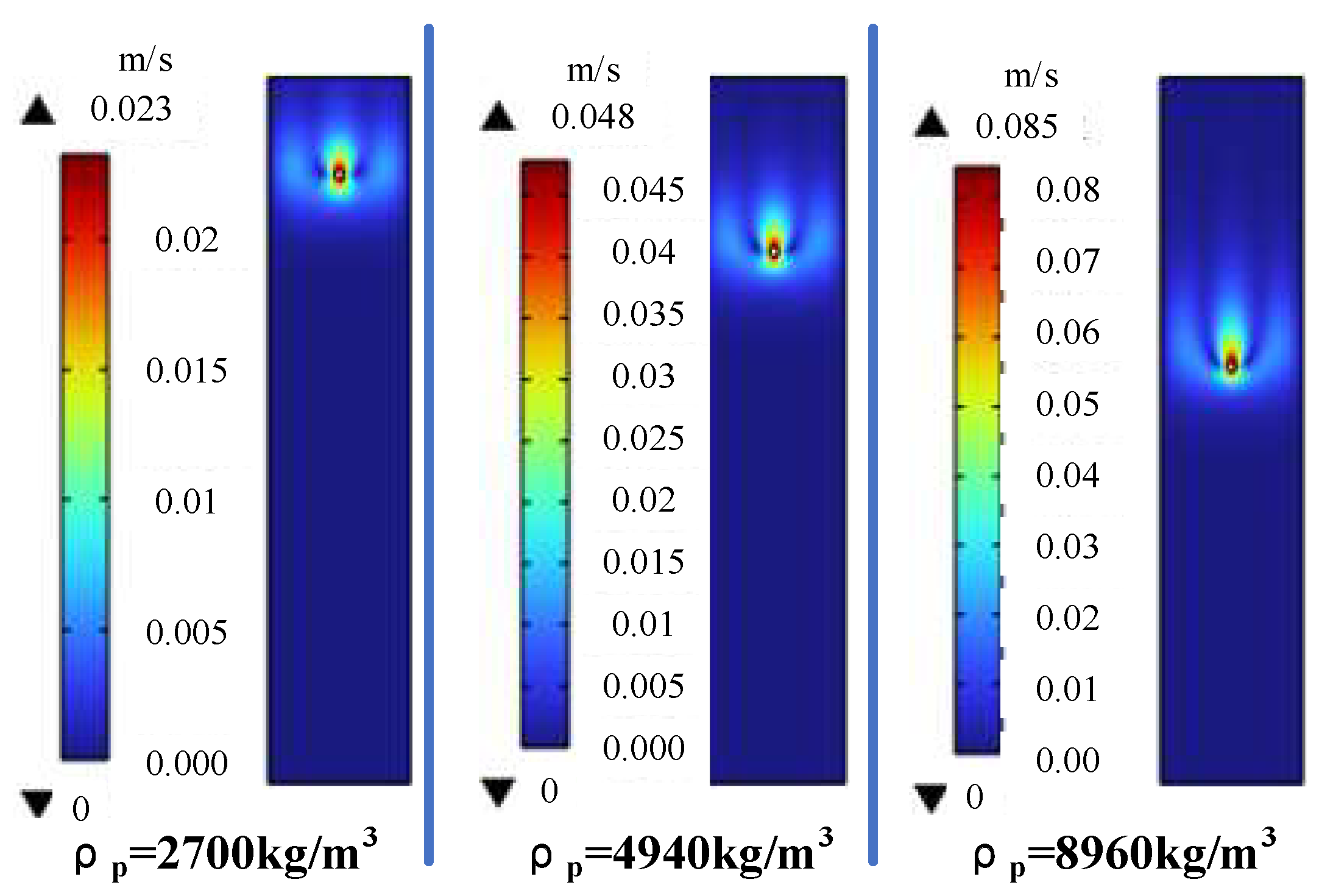
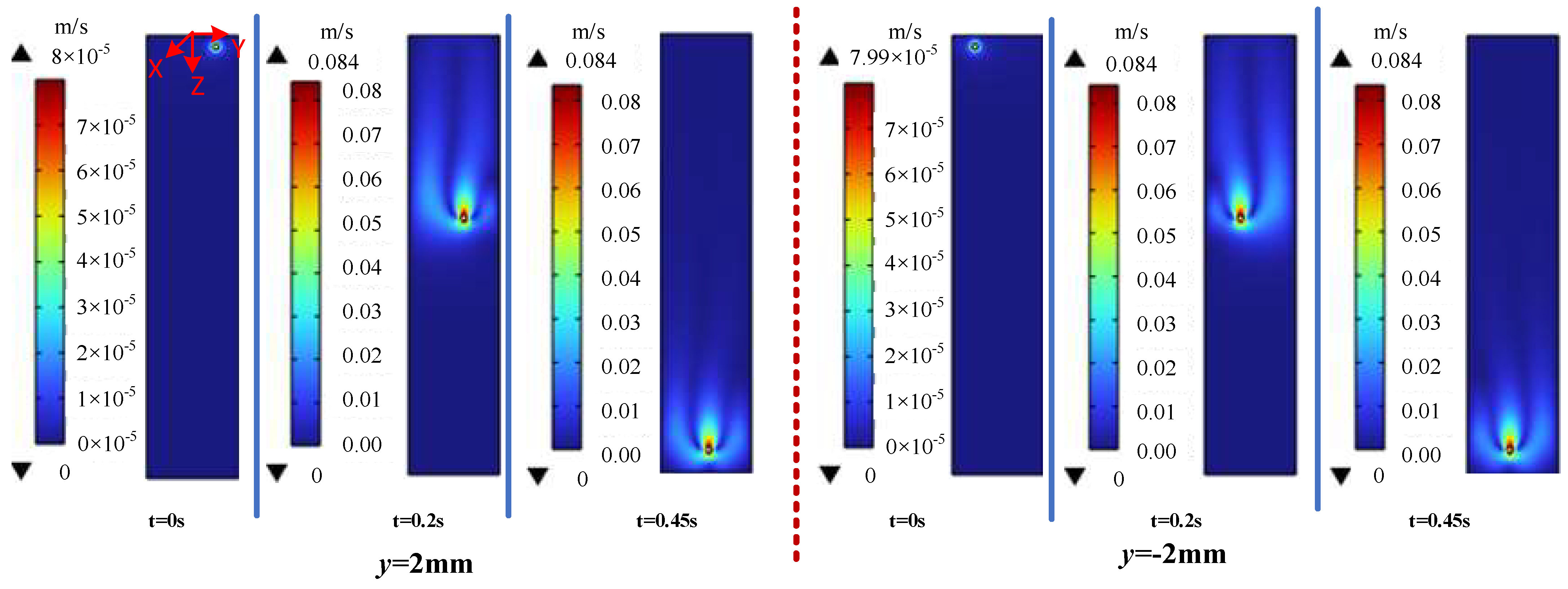
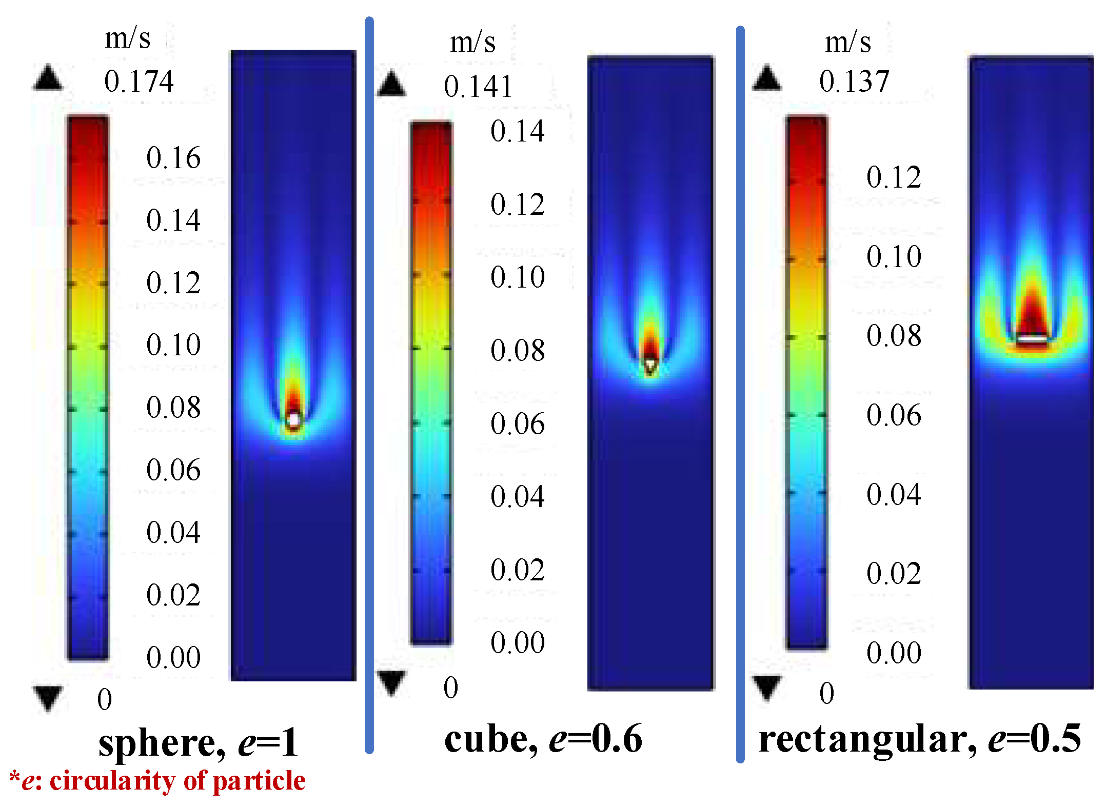
3.2. Numerical Study Results
3.3. Inline Monitoring Sensor Design
3.4. Experimental Study Results
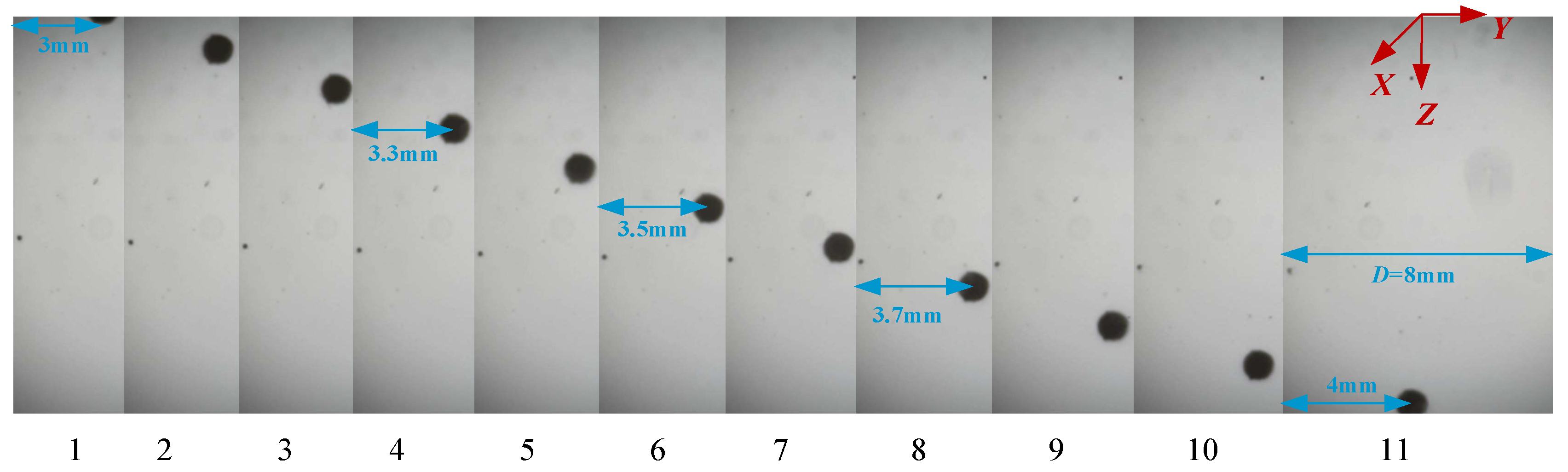
3.4.1. Velocity Measurement of the Particles
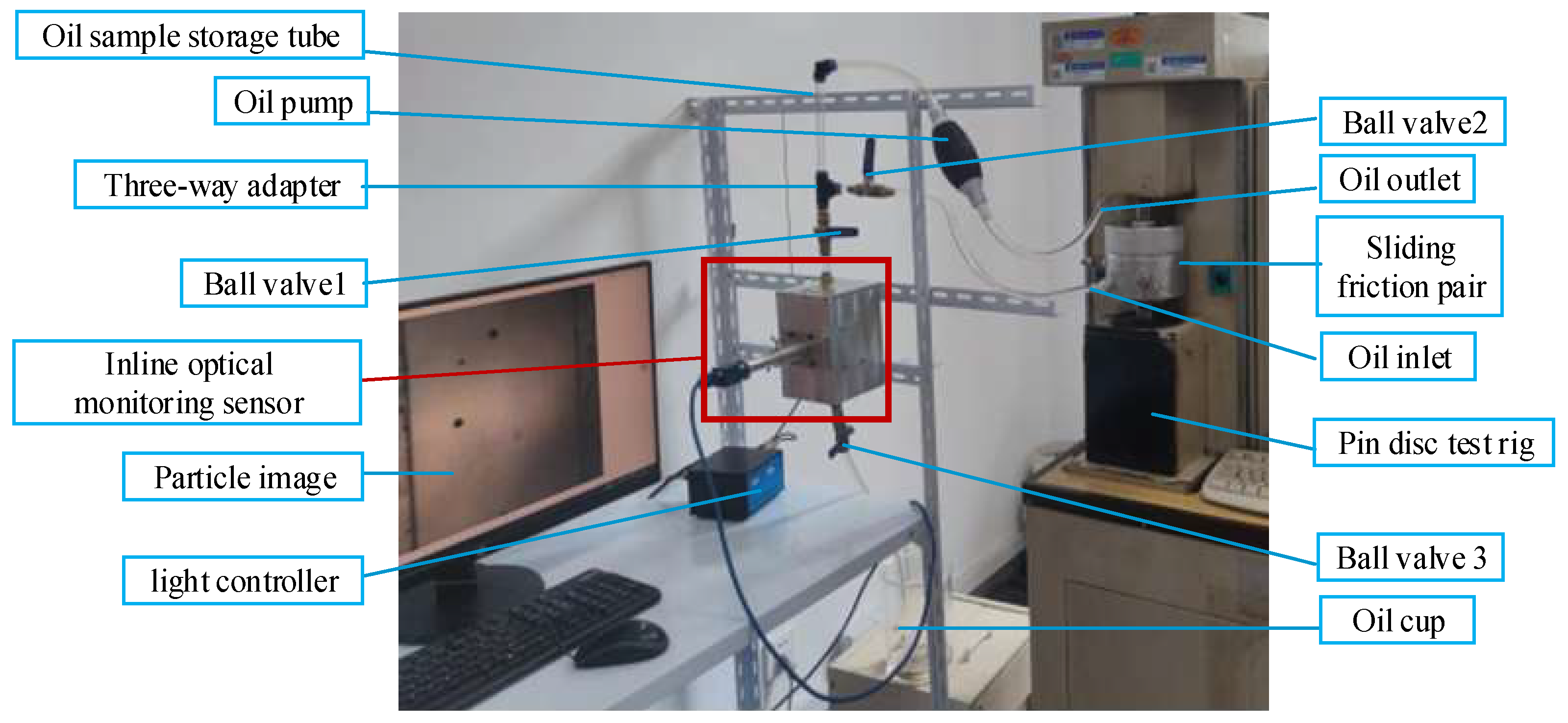
3.4.2. Experimental System
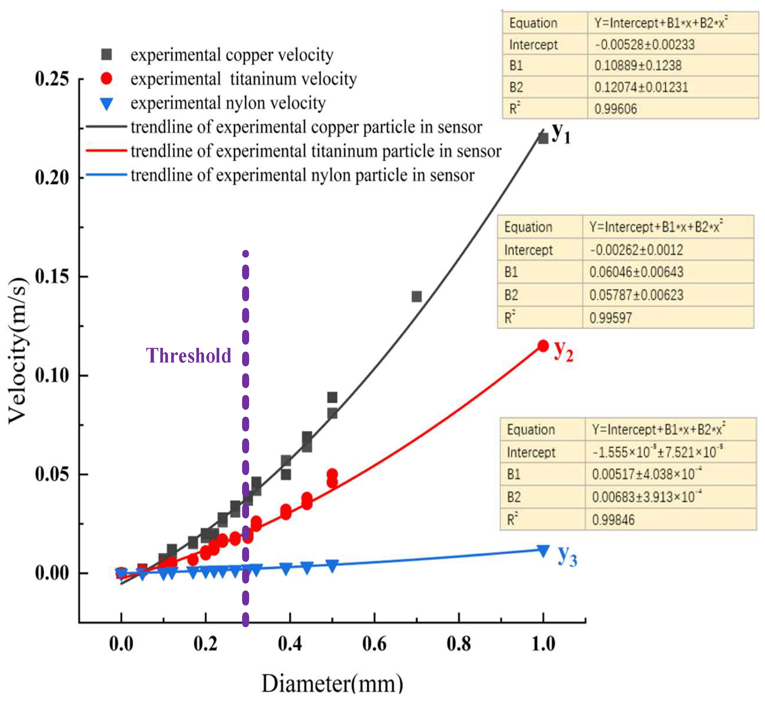
3.4.3. Experimental Results
3.4.4. Monitoring Model
3.5. Discussion
4. Conclusions
Author Contributions
Funding
Institutional Review Board Statement
Informed Consent Statement
Data Availability Statement
Conflicts of Interest
Nomenclature
| Symbol | Unit | Description |
| Particle size | ||
| g | Gravitational acceleration | |
| d | Pipe diameter | |
| L | Pipe length | |
| Particle density | ||
| Oil density | ||
| / | Drag coefficient | |
| Particle movement velocity | ||
| Free settling velocity of a single solid sphere in an unbounded fluid | ||
| Fluid flow rate | ||
| Kinematic viscosity coefficient of oil | ||
| Dynamic viscosity coefficient of oil | ||
| Time | ||
| Gravity | ||
| Buoyancy | ||
| Drag force | ||
| Additional mass force | ||
| Basset force | ||
| Saffman lifting force | ||
| / | Particle Reynolds number | |
| Particle movement velocity | ||
| Pressure | ||
| The velocity component of the fluid at time direction | ||
| The external force per unit volume of fluid in the direction | ||
| Particle image pixel area | ||
| e | / | Circularity of particle |
References
- Lu, P.; Powrie, H.E.; Wood, R.J.K.; Harvey, T.J.; Harris, N.R. Early wear detection and its significance for condition monitoring. Tribol. Int. 2021, 159, 106946. [Google Scholar] [CrossRef]
- Li, D.; Zhang, M.; Kang, T.; Li, B.; Xiang, H.; Wang, K.; Pei, Z.; Tang, X.; Wang, P. Fault diagnosis of rotating machinery based on dual convolutional-capsule network (DC-CN). Measurement 2022, 187, 110258. [Google Scholar] [CrossRef]
- Li, Y.; Zou, W.; Jiang, L. Fault diagnosis of rotating machinery based on combination of Wasserstein generative adversarial networks and long short term memory fully convolutional network. Measurement 2022, 191, 110826. [Google Scholar] [CrossRef]
- Ravikumar, K.N.; Yadav, A.; Kumar, H.; Gangadharan, K.V.; Narasimhadhan, A.V. Gearbox fault diagnosis based on Multi-Scale deep residual learning and stacked LSTM model. Measurement 2021, 186, 110099. [Google Scholar] [CrossRef]
- Tang, M.; Liao, Y.; He, D.; Duan, R.; Zhang, X. Rolling bearing diagnosis based on an unbiased-autocorrelation morphological filter method. Measurement 2022, 189, 110617. [Google Scholar] [CrossRef]
- Tao, L.; Sun, L.; Wu, Y.; Lu, C.; Ma, J.; Cheng, Y.; Suo, M. Multi-signal fusion diagnosis of gearbox based on minimum Bayesian risk reclassification and adaptive weighting. Measurement 2022, 187, 110358. [Google Scholar] [CrossRef]
- Yao, Y.; Gui, G.; Yang, S.; Zhang, S. An adaptive anti-noise network with recursive attention mechanism for gear fault diagnosis in real-industrial noise environment condition. Measurement 2021, 186, 110169. [Google Scholar] [CrossRef]
- Cheng, C.; Ma, G.; Zhang, Y.; Sun, M.; Teng, F.; Ding, H.; Yuan, Y. A Deep Learning-Based Remaining Useful Life Prediction Approach for Bearings. IEEE/ASME Trans. Mechatron. 2020, 25, 1243–1254. [Google Scholar] [CrossRef]
- Wang, J.; Wang, G.; Cheng, L. Texture extraction of wear particles based on improved random Hough transform and visual saliency. Eng. Fail. Anal. 2020, 109, 104299. [Google Scholar] [CrossRef]
- Hong, W.; Cai, W.; Wang, S.; Tomovic, M.M. Mechanical wear debris feature, detection, and diagnosis: A review. Chin. J. Aeronaut. 2018, 31, 867–882. [Google Scholar] [CrossRef]
- Liu, R.; Bei, S.; Gu, M.; Wang, H.; Sun, J. Research on Characteristics of Electrostatic Wear-Site and Oil-Line Sensor with Theoretical and Comprehensive Analysis. J. Sens. 2022, 2022, 9188776. [Google Scholar] [CrossRef]
- Guerrero, J.M.; Castilla, A.E.; Fernandez, J.A.S.; Platero, C.A. Transformer Oil Diagnosis Based on a Capacitive Sensor Frequency Response Analysis. IEEE Access 2021, 9, 7576–7585. [Google Scholar] [CrossRef]
- Yu, B.; Cao, N.; Zhang, T. A novel signature extracting approach for inductive oil debris sensors based on symplectic geometry mode decomposition. Measurement 2021, 185, 110056. [Google Scholar] [CrossRef]
- Liu, Z.; Liu, Y.; Zuo, H.; Wang, H.; Wang, C. Oil debris and viscosity monitoring using optical measurement based on Response Surface Methodology. Measurement 2022, 195, 111152. [Google Scholar] [CrossRef]
- Jia, R.; Wang, L.; Zheng, C.; Chen, T. Online Wear Particle Detection Sensors for Wear Monitoring of Mechanical Equipment—A Review. IEEE Sens. J. 2022, 22, 2930–2947. [Google Scholar] [CrossRef]
- Fan, H.; Gao, S.; Zhang, X.; Cao, X.; Ma, H.; Liu, Q. Intelligent Recognition of Ferrographic Images Combining Optimal CNN with Transfer Learning Introducing Virtual Images. IEEE Access 2020, 8, 137074–137093. [Google Scholar] [CrossRef]
- Wang, J.; Bi, J.; Wang, L.; Wang, X. A non-reference evaluation method for edge detection of wear particles in ferrograph images. Mech. Syst. Signal Processing 2018, 100, 863–876. [Google Scholar] [CrossRef]
- Feng, S.; Qiu, G.; Luo, J.; Han, L.; Mao, J.; Zhang, Y. A Wear Debris Segmentation Method for Direct Reflection Online Visual Ferrography. Sensors 2019, 19, 723. [Google Scholar] [CrossRef]
- Wu, T.; Wu, H.; Du, Y.; Peng, Z. Progress and trend of sensor technology for on-line oil monitoring. Sci. China Technol. Sci. 2013, 56, 2914–2926. [Google Scholar] [CrossRef]
- Liu, Z.; Liu, Y.; Zuo, H.; Wang, H.; Fei, H. A Lubricating Oil Condition Monitoring System Based on Wear Particle Kinematic Analysis in Microfluid for Intelligent Aeroengine. Micromachines 2021, 12, 748. [Google Scholar] [CrossRef]
- Peng, Y.; Wu, T.; Wang, S.; Du, Y.; Kwok, N.; Peng, Z. A microfluidic device for three-dimensional wear debris imaging in online condition monitoring. Proc. Inst. Mech.Eng. Part J J. Eng. Tribol. 2016, 231, 965–974. [Google Scholar] [CrossRef]
- Feng, S.; Zeng, Q.H.; Fan, B.; Luo, J.F.; Xiao, H.; Mao, J.H. Wear Debris Segmentation of Reflection Ferrograms Using Lightweight Residual U-Net. IEEE Trans. Instrum. Meas. 2021, 70, 3099573. [Google Scholar] [CrossRef]
- Peng, P.; Wang, J.G. FECNN: A promising model for wear particle recognition. Wear 2019, 432, 202968. [Google Scholar] [CrossRef]
- Segré, G.; Silberberg, A. Behaviour of macroscopic rigid spheres in Poiseuille flow Part 2. Experimental results and interpretation. J. Fluid Mech. 2006, 14, 136–157. [Google Scholar] [CrossRef]
- Jeffrey, R.C.; Pearson, J.R.A. Particle motion in laminar vertical tube flow. J. Fluid Mech. 2006, 22, 721–735. [Google Scholar] [CrossRef]
- Shehua, H.; Wei, L.; Liangjun, C. On equation of discrete solid particles’ motion in arbitrary flow field and its properties. Appl. Math. Mech. 2000, 21, 297. [Google Scholar] [CrossRef]
- Choi, H.M.; Kurihara, T.; Monji, H.; Matsui, G. Measurement of particle/bubble motion and turbulence around it by hybrid PIV. Flow Meas. Instrum. 2002, 12, 421–428. [Google Scholar] [CrossRef]
- Miura, K.; Itano, T.; Sugihara-Seki, M. Inertial migration of neutrally buoyant spheres in a pressure-driven flow through square channels. J. Fluid Mech. 2014, 749, 320–330. [Google Scholar] [CrossRef]
- Oseen, C.W. Neuere Methoden Und Ergebnisse in Der Hydrodynamik; Akademische Verlagsgesellschaft: Leipzig, Germany, 1927. [Google Scholar]
- Barton, I.E. Computation of particle tracks over a backward-facing step. J. Aerosol Sci. 1995, 26, 887–901. [Google Scholar] [CrossRef]
- Fan, L.; Zhu, C. Momentum Transfer and Charge Transfer. In Principles of Gas-Solid Flows; Cambridge Series in Chemical Engineering; Cambridge University Press: Cambridge, UK, 1998; pp. 87–129. [Google Scholar]
- Hedayati Nasab, S. Free Falling of Spheres in a Quiescent Fluid. 2017. Available online: https://spectrum.library.concordia.ca/id/eprint/983050/ (accessed on 1 September 2021).
- Sun, J.; Wang, L.; Li, J.; Li, F.; Li, J.; Lu, H. Online oil debris monitoring of rotating machinery: A detailed review of more than three decades. Mech. Syst. Signal Processing 2021, 149, 107341. [Google Scholar] [CrossRef]
- Yang, X. The Motion of the Particles in Simple Flows Using the Lattice Boltzmann Method; University of Science and Technology of China: Hefei, China, 2016. [Google Scholar]
- Aidun, C.K.; Lu, Y.; Ding, E.J. Direct analysis of particulate suspensions with inertia using the discrete Boltzmann equation. J. Fluid Mech. 1998, 373, 287–311. [Google Scholar] [CrossRef]
- Peng, P.; Wang, J. Wear particle classification considering particle overlapping. Wear 2019, 422–423, 119–127. [Google Scholar] [CrossRef]


| Shape | Diameter (mm) | Density (kg/m3) | Material | Width (mm) | Height (mm) | Circularity |
|---|---|---|---|---|---|---|
| round | 1 | 8960 | copper | / | 1 | |
| 0.5 | / | 1 | ||||
| 0.1 | / | 1 | ||||
| 0.5 | 4940 | titanium | / | 1 | ||
| 0.5 | 2700 | aluminum | / | 1 | ||
| triangle | / | 8960 | copper | 1 | 1 | 0.6 |
| square | / | 8960 | copper | 1 | 0.2 | 0.5 |
| Test Material | Copper | Titanium | Nylon |
|---|---|---|---|
| Density (kg/m3) | 8900 | 4500 | 1150 |
Publisher’s Note: MDPI stays neutral with regard to jurisdictional claims in published maps and institutional affiliations. |
© 2022 by the authors. Licensee MDPI, Basel, Switzerland. This article is an open access article distributed under the terms and conditions of the Creative Commons Attribution (CC BY) license (https://creativecommons.org/licenses/by/4.0/).
Share and Cite
Liu, Z.; Liu, Y.; Zuo, H.; Wang, H.; Chen, Z. An Oil Wear Particles Inline Optical Sensor Based on Motion Characteristics for Rotating Machines Condition Monitoring. Machines 2022, 10, 727. https://doi.org/10.3390/machines10090727
Liu Z, Liu Y, Zuo H, Wang H, Chen Z. An Oil Wear Particles Inline Optical Sensor Based on Motion Characteristics for Rotating Machines Condition Monitoring. Machines. 2022; 10(9):727. https://doi.org/10.3390/machines10090727
Chicago/Turabian StyleLiu, Zhenzhen, Yan Liu, Hongfu Zuo, Han Wang, and Zhixiong Chen. 2022. "An Oil Wear Particles Inline Optical Sensor Based on Motion Characteristics for Rotating Machines Condition Monitoring" Machines 10, no. 9: 727. https://doi.org/10.3390/machines10090727