
A Holistic Approach to IGBT Board Surface Fractal Object Detection Based on the Multi-Head Model

Abstract
:1. Introduction
- The IWS (Information Watch and Study module) module (Section 3.1) was proposed by us to increase the detection dimension of object information;
- We designed the FGI (Fine-Grained Information) Head (Section 3.1.1) to extract more comprehensive feature vectors. For object information calculation and class cluster center learning, we proposed a WST (Watch and Study Tactic) Learner (Section 3.1.2);
- The MRD (Multi-task Result Determination) strategy (Section 3.1.3) that combines classification information and fine-grained information to give detection results were designed. We proposed an adjustment mechanism of class learning weights (Section 3.3). Its goal is to force the network model to fully learn the characteristics of each class. A new evaluation index (Section 3.2) was designed to facilitate better judgment.
2. Related Work
2.1. Object Detection
2.2. Fractal Object Recognition
3. Methodology
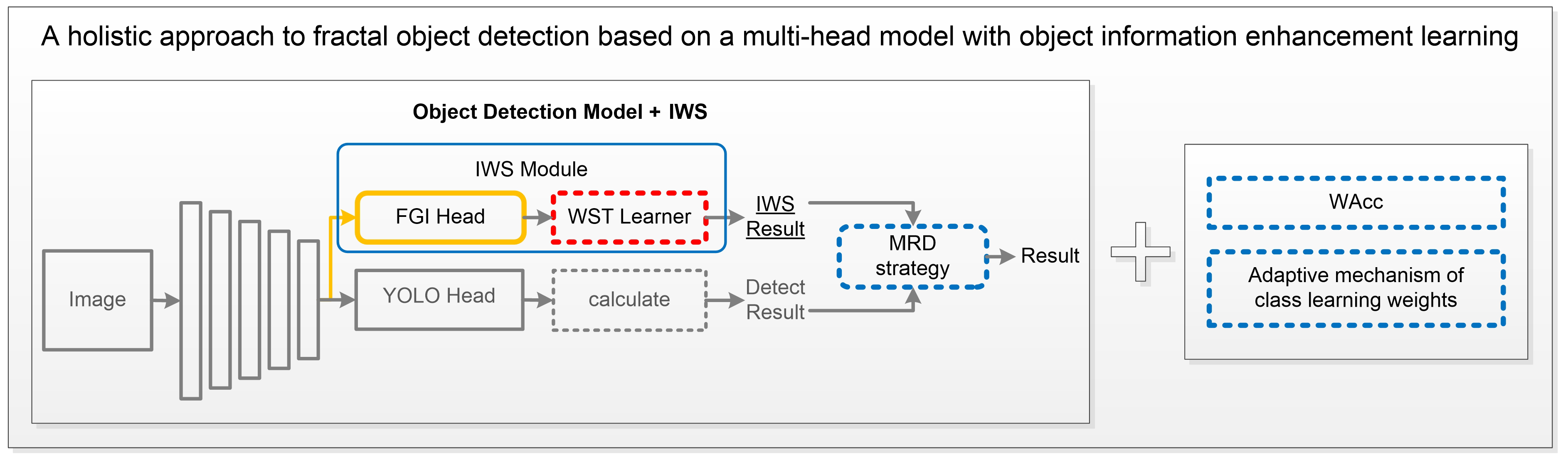
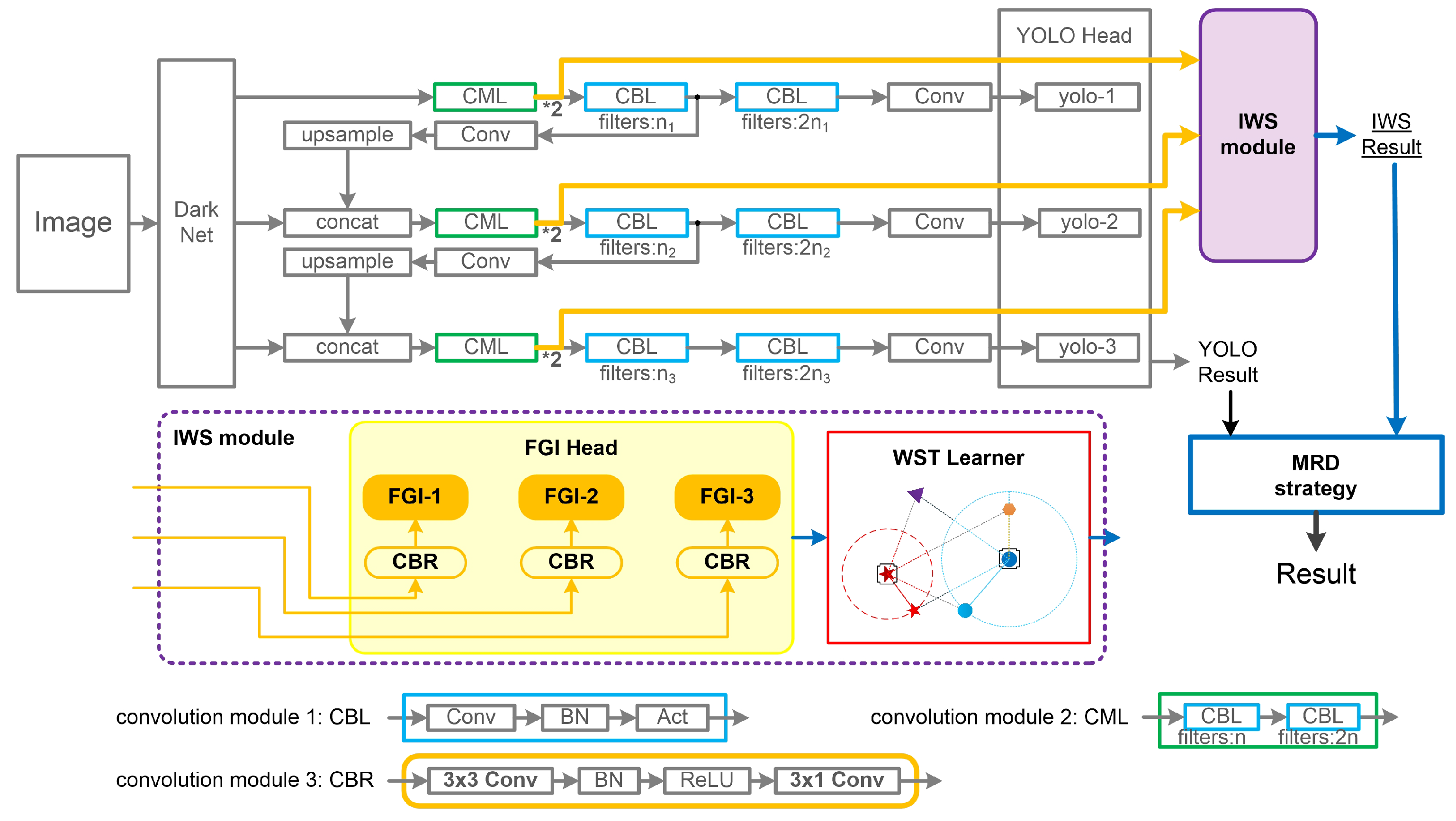
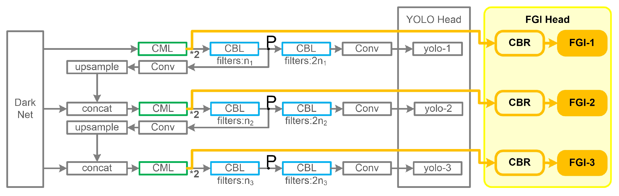
3.1. YOLO with IWS
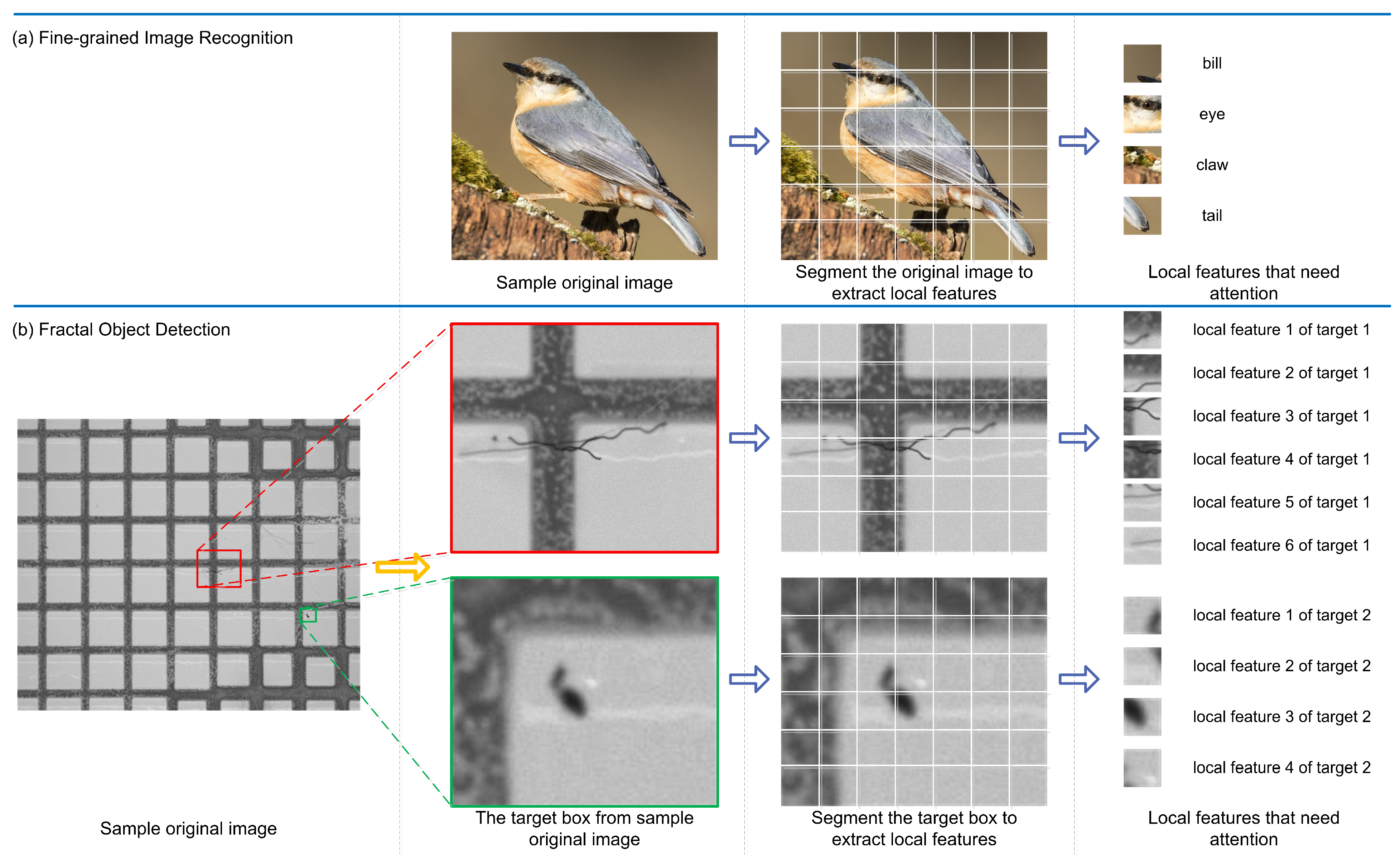
3.1.1. FGI Head
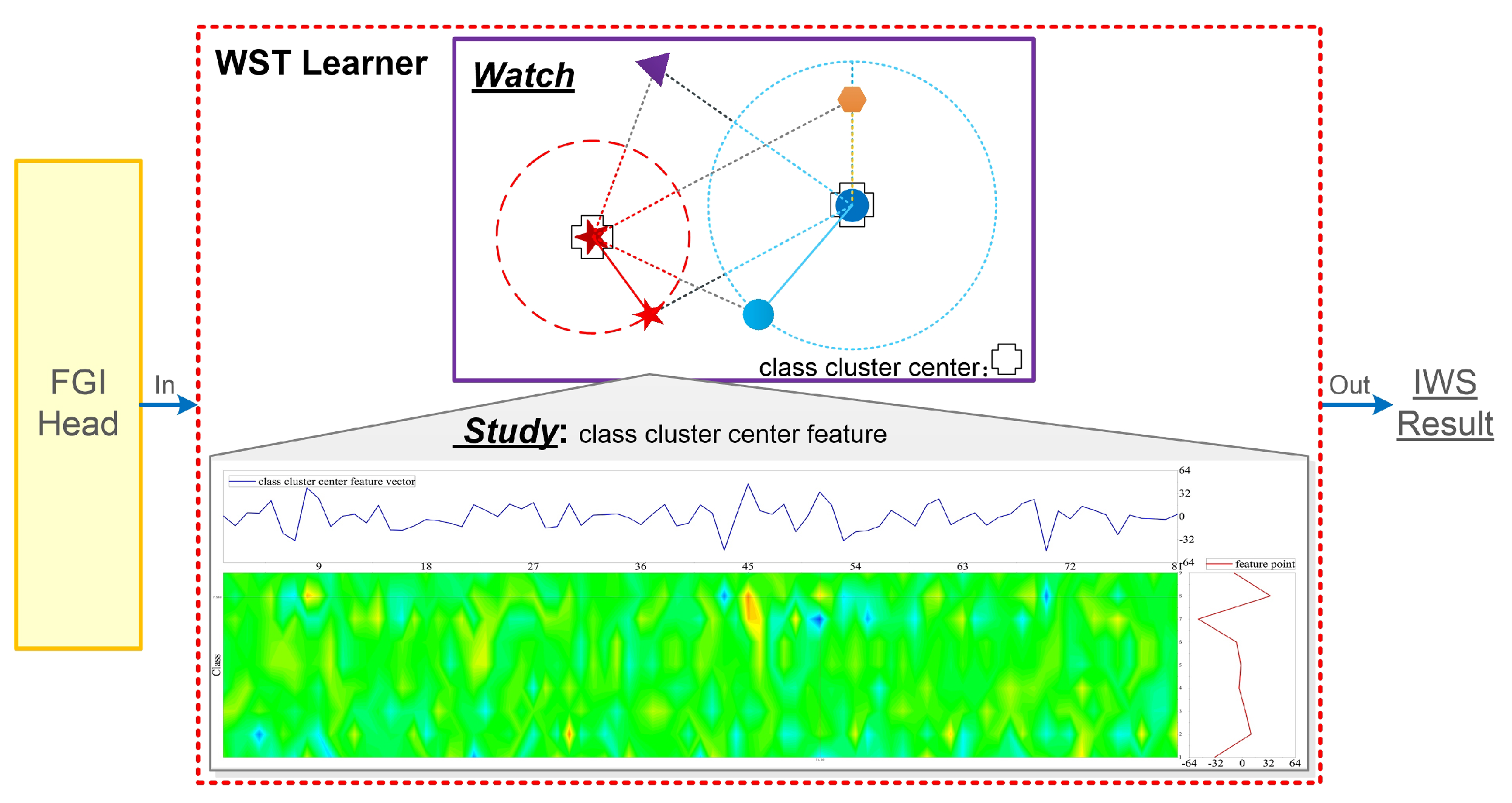
3.1.2. WST Learner
| Algorithm 1 WST Learner in training phase. |
| Input: batch number , class number , the number of feature vectors belonging to class k is , class cluster centre feature vector , feature number , feature vector x |
| Output: WST Loss |
| 1: if then |
| 2: Initialize |
| 3: else |
| 4: if then |
| 5: |
| 6: else |
| 7: and Equation (3) |
| 8: end if |
| 9: end if |
| 10: and Equation (1) |
| 11: and Equation (5) |
| 12: return |
3.1.3. Multi-Task Result Discriminant Strategy
| Algorithm 2 Multi-Task Result Discriminant strategy. |
| Input: candidate results of the IWS module for object i are , , result of the YOLO classier is |
| Output: result of the model classier is |
| 1: if then |
| 2: if then |
| 3: if then |
| 4: new or unkonw class. Classify i as novelty samples |
| 5: else |
| 6: |
| 7: end if |
| 8: else |
| 9: if then |
| 10: Classify i as hard samples |
| 11: end if |
| 12: |
| 13: end if |
| 14: else |
| 15: if then |
| 16: if then |
| 17: new or unkonw class. Classify i as novelty samples |
| 18: else |
| 19: . Classify i as hard samples |
| 20: end if |
| 21: else |
| 22: if then. Classify i as hard samples |
| 23: end if |
| 24: |
| 25: end if |
| 26: end if |
| 27: return |
3.2. WST Accuracy (WAcc)
3.3. Adjustment Mechanism of Class Learning Weights
| Algorithm 3 Adjustment mechanism. |
| Input: class weights , class Loss , epoch size T, epoch number , momentum parameter of class learning is |
| Output:W |
| 1: if then |
| 2: Initialize and |
| 3: end if |
| 4: if then |
| 5: |
| 6: |
| 7: |
| 8: end if |
| 9: return W |
4. Approach
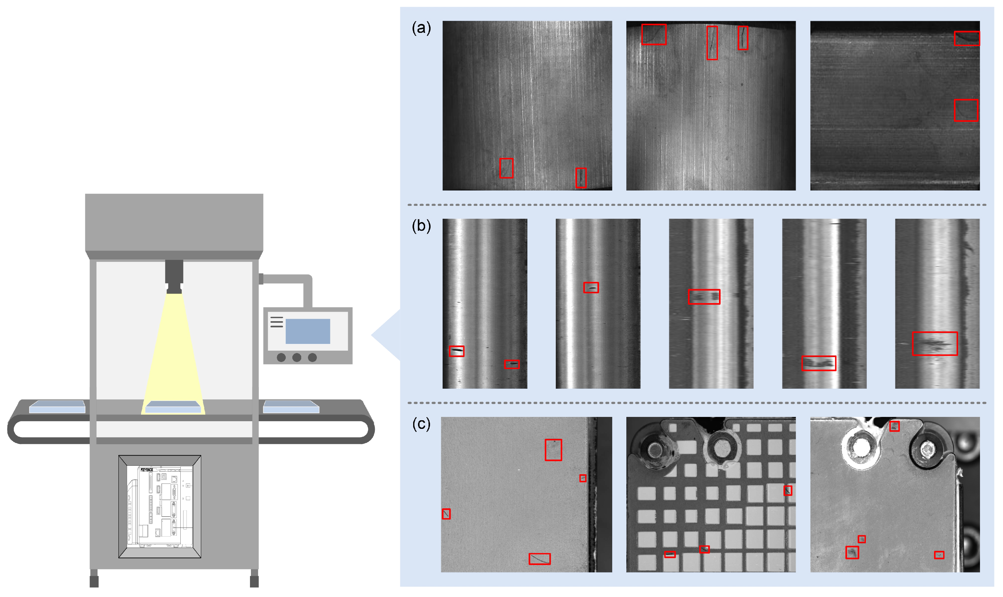
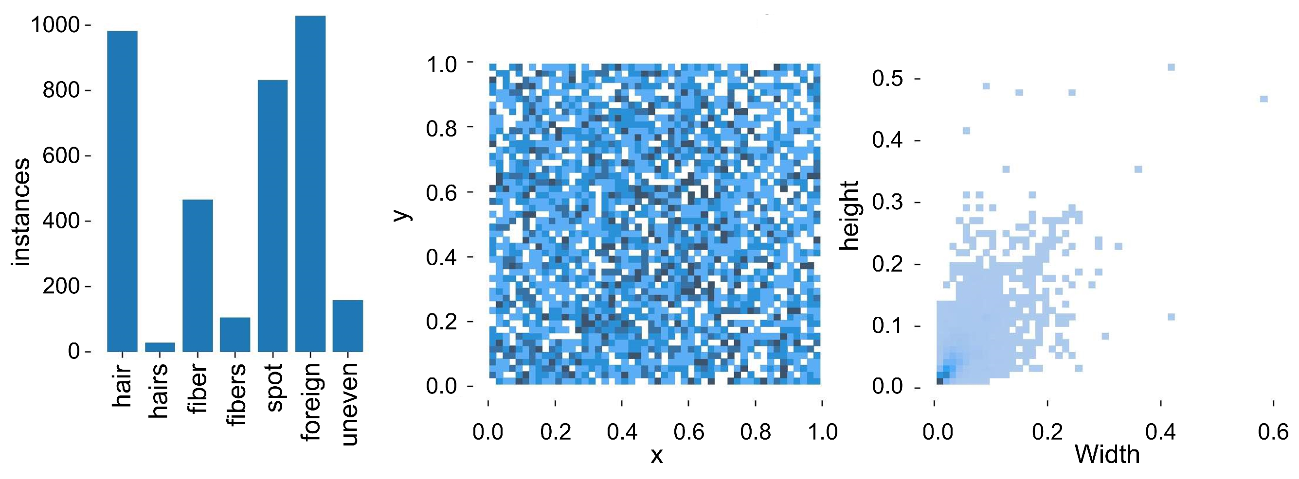
4.1. Experimental Dataset
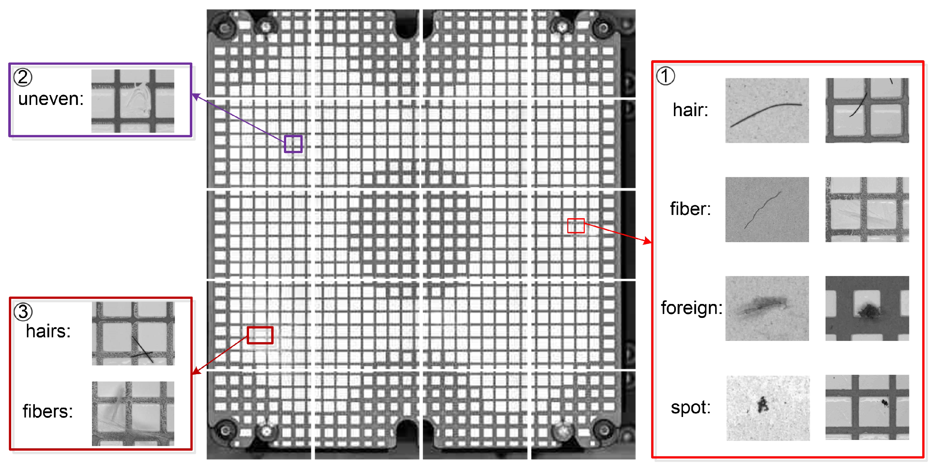
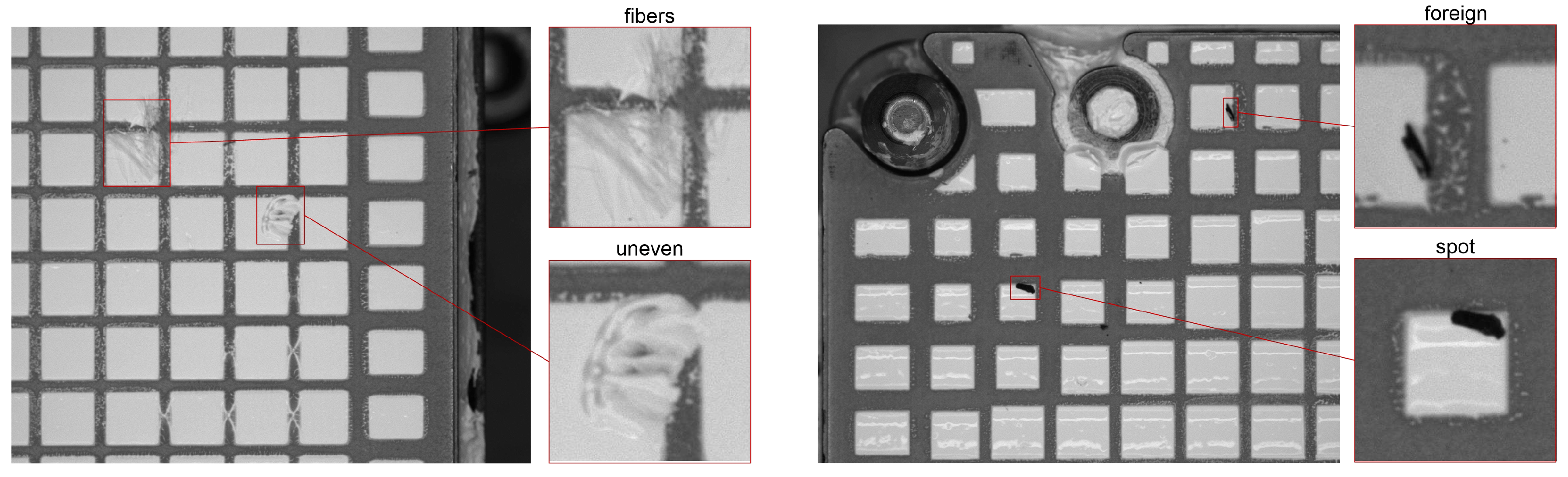
- Common foreign object collection, including hair, fiber, packaging crumbs (foreign), and object crumbs (spot) are used for learning characteristics of common fractal objects. The main learning sample of the fractal object detectability for the dust-free future provides information support for the management and control of bacteria in the workspace (shown as ① in Figure 8). The purpose of doing this is not only to detect whether it is a foreign object, but also what kind of foreign object it is. So we need a multi-class classification dataset, not a binary classification dataset.
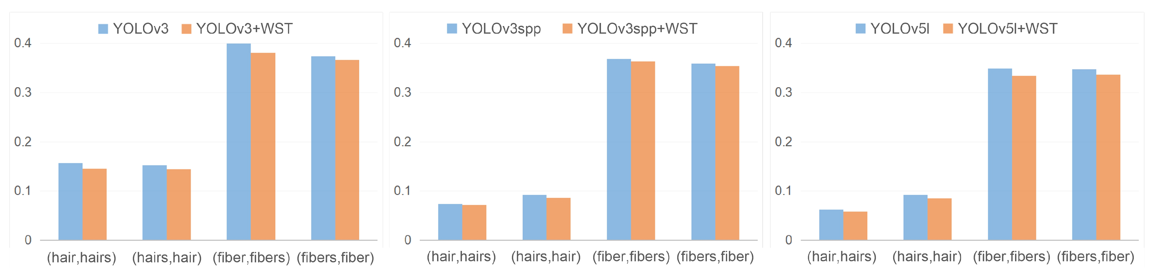
- Glue application collection, including uneven glue application (shown as ② in Figure 8). Since foreign and spot are similar, fiber and uneven are also difficult to distinguish (due to low contrast). We used foreign and spot, fiber and uneven as the main fractal object detection groups;
- The collection of complex objects, including cross hairs and fibers, is used to learn the characteristics of objects and enhance the model detectability (shown as ③ in Figure 8). Whether the detection network can effectively detect when the number of fractal objects changes in complex situations is investigated.
4.2. Evaluation Metrics
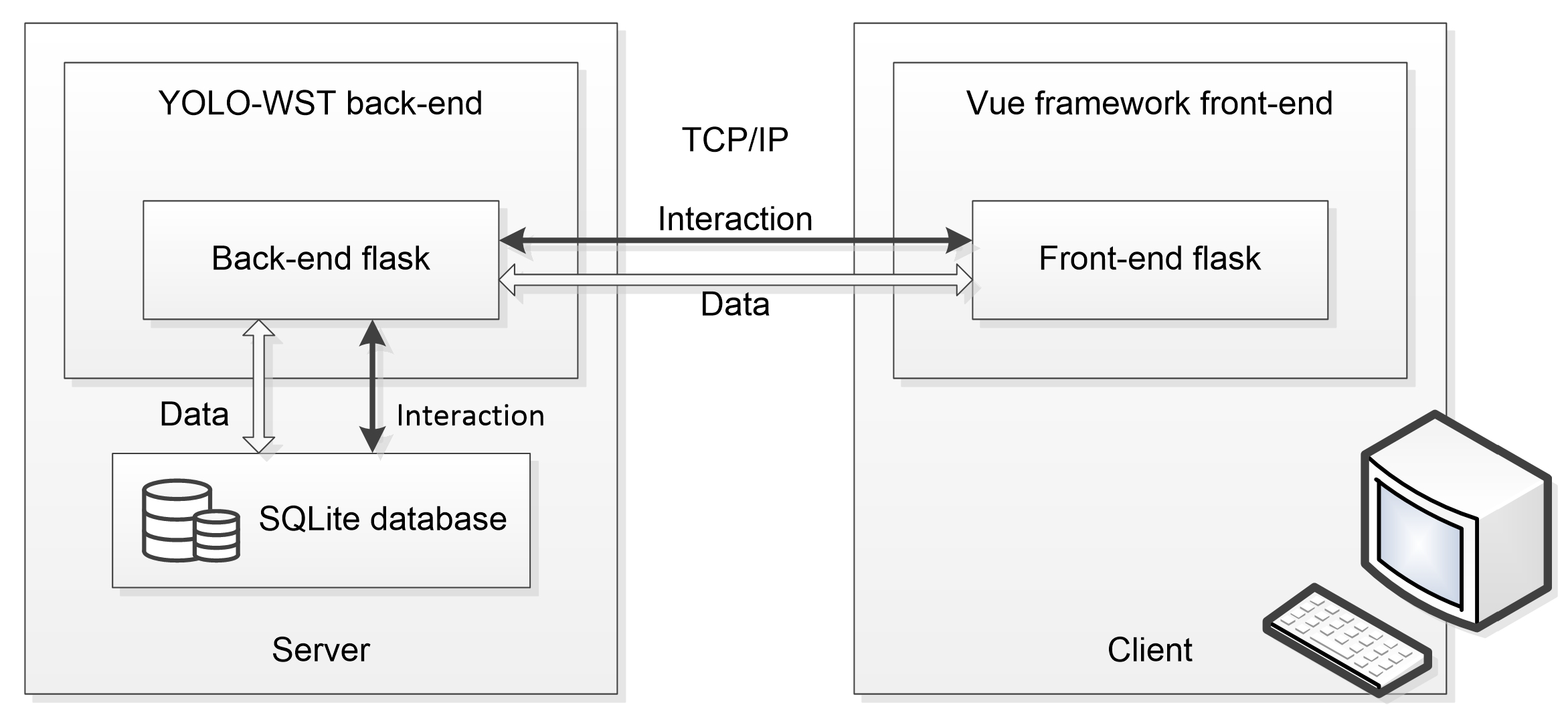
4.3. Experimental Apparatus
4.4. Implementation Details
5. Results and Discussion
5.1. Experimental Analysis with Industrial Visual Inspection Data
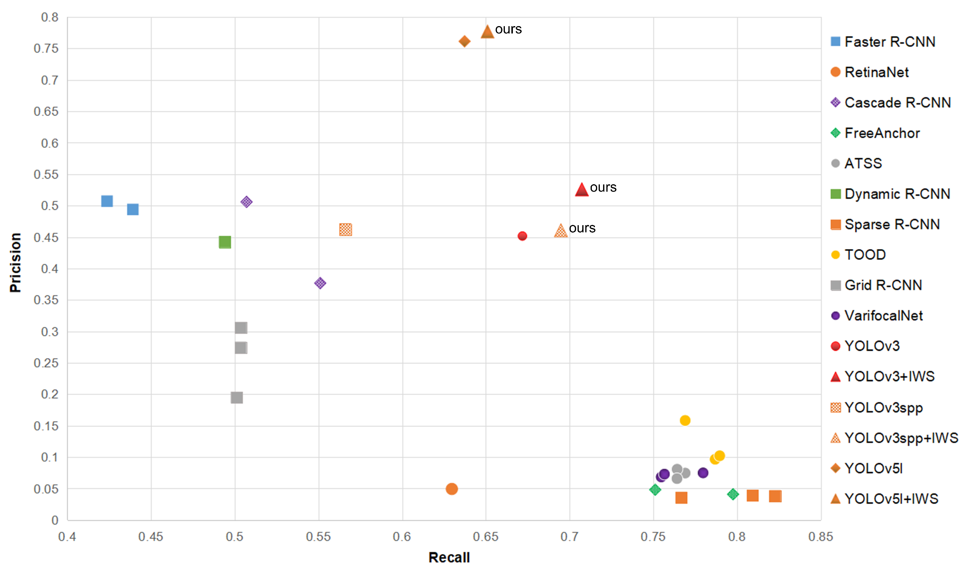
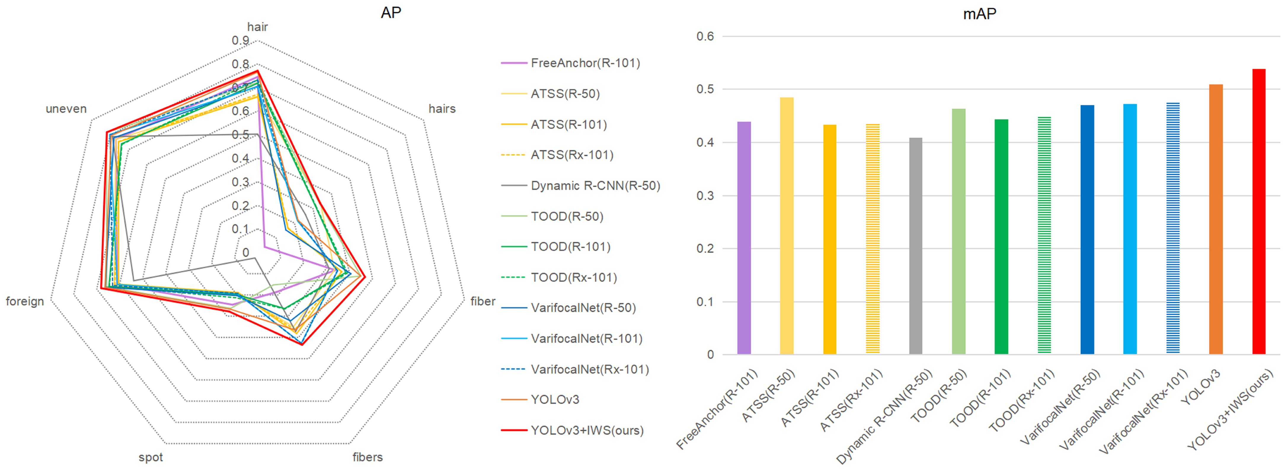
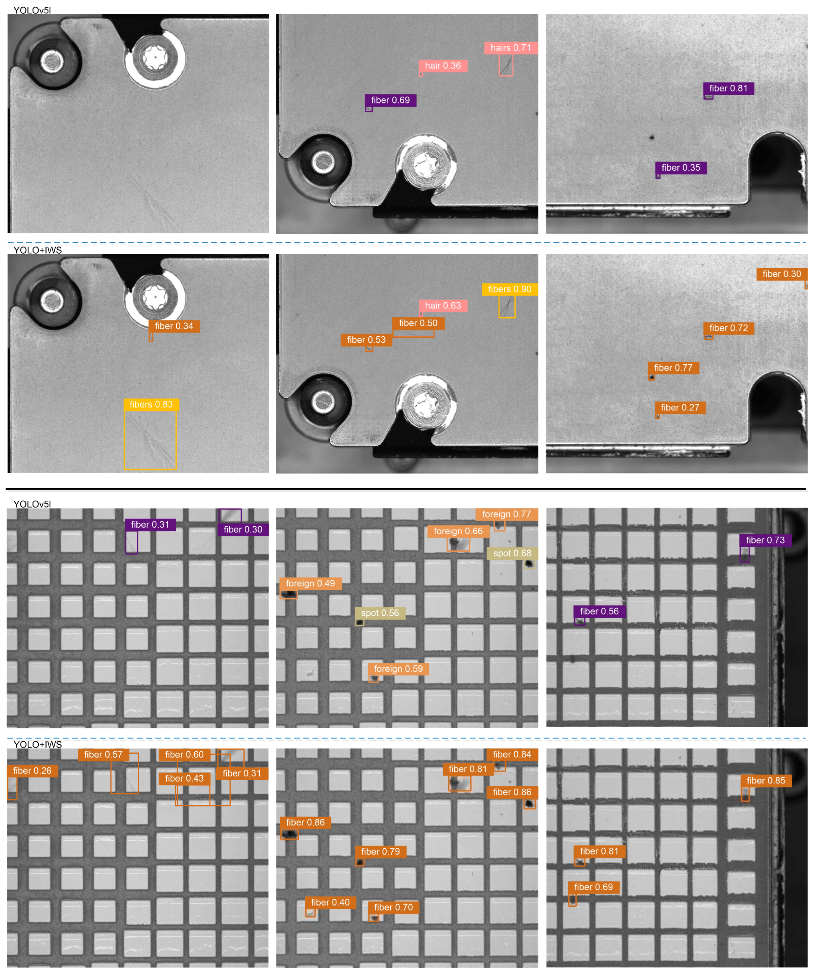
5.1.1. Compared with State-of-the-Art Approaches
5.1.2. Portability
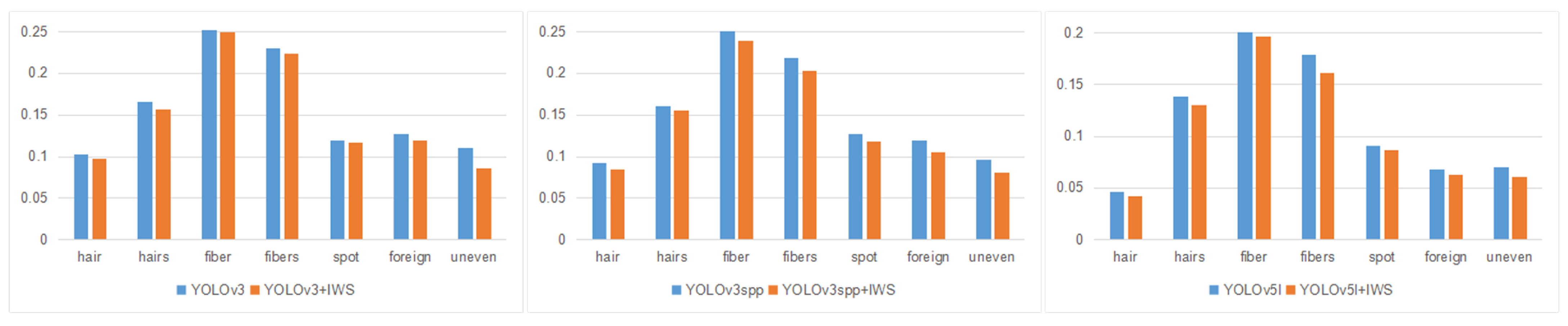
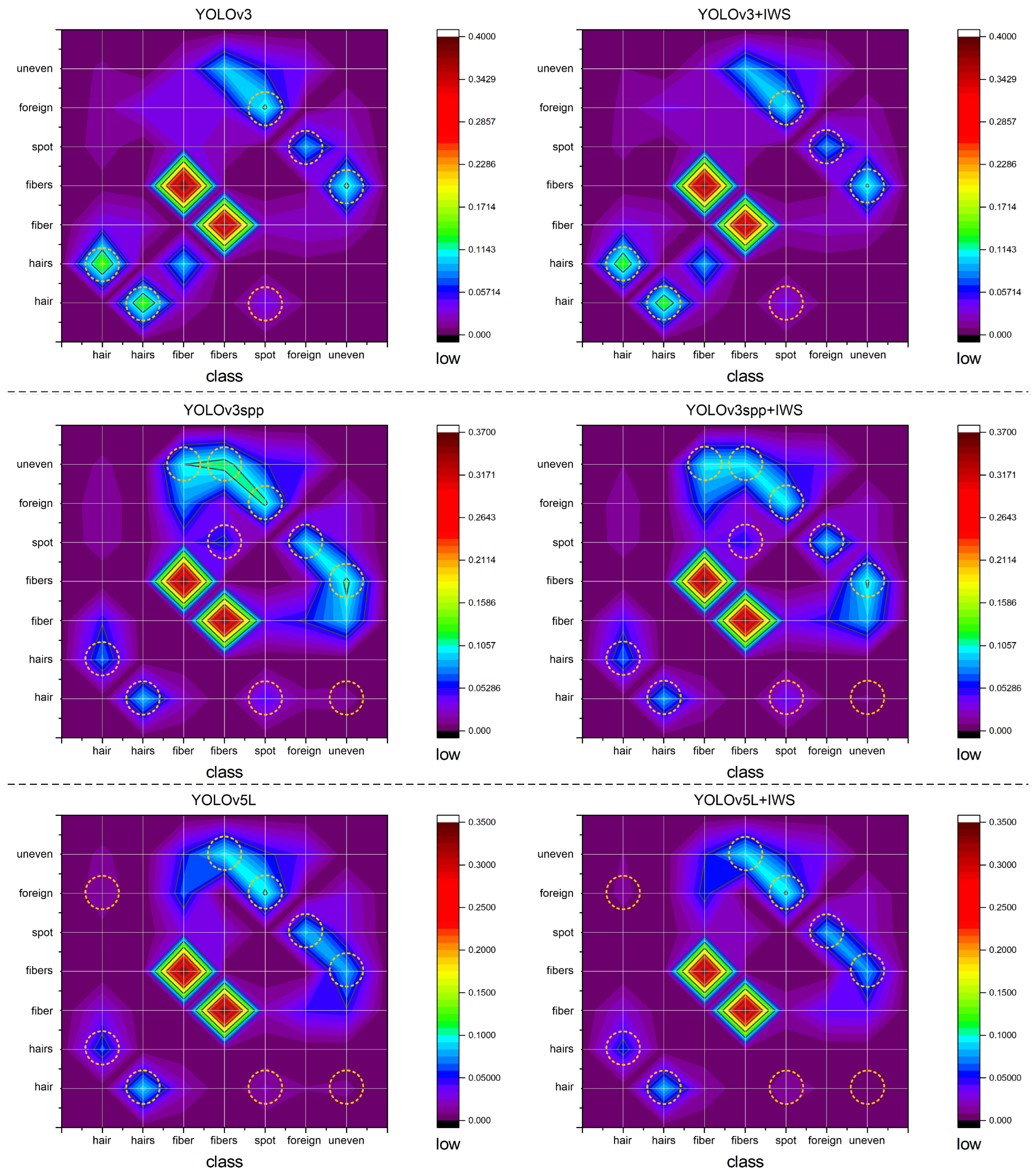
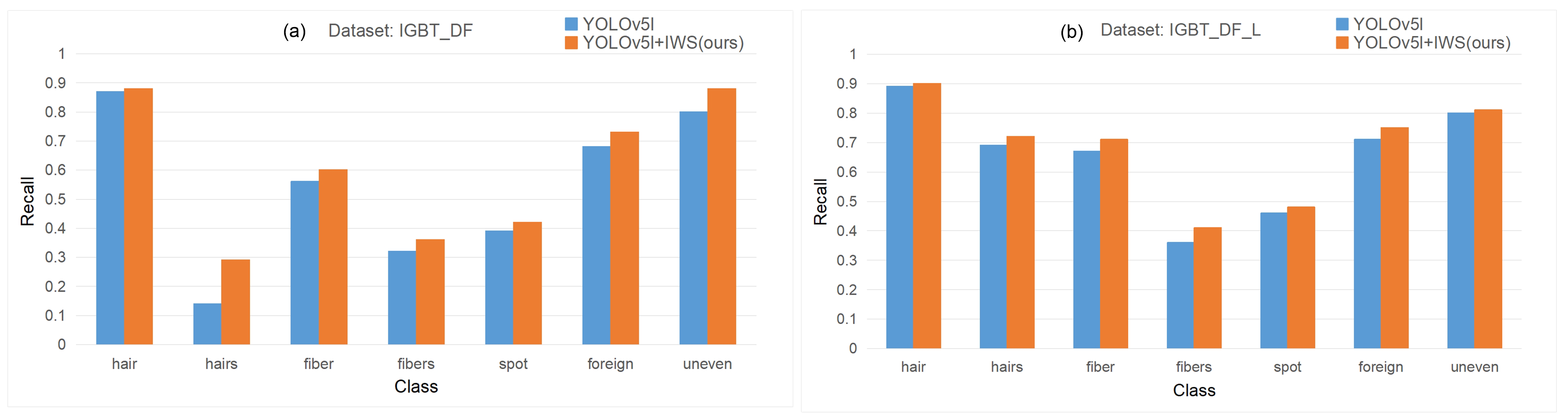
5.1.3. Experiment Details for Each Class of Fractal Objects
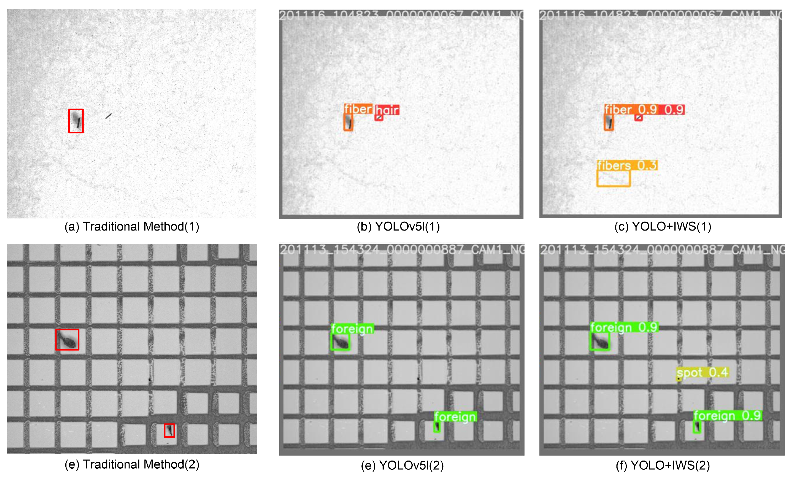
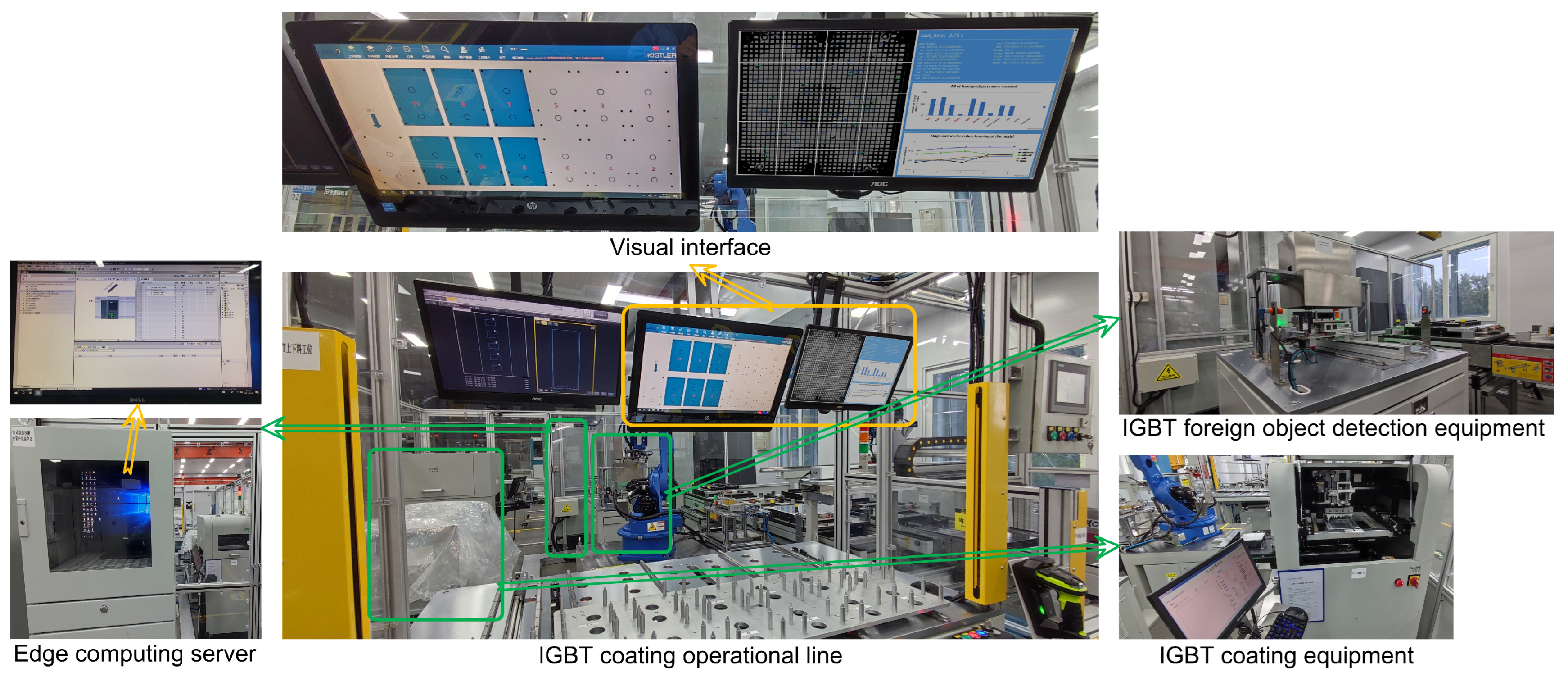
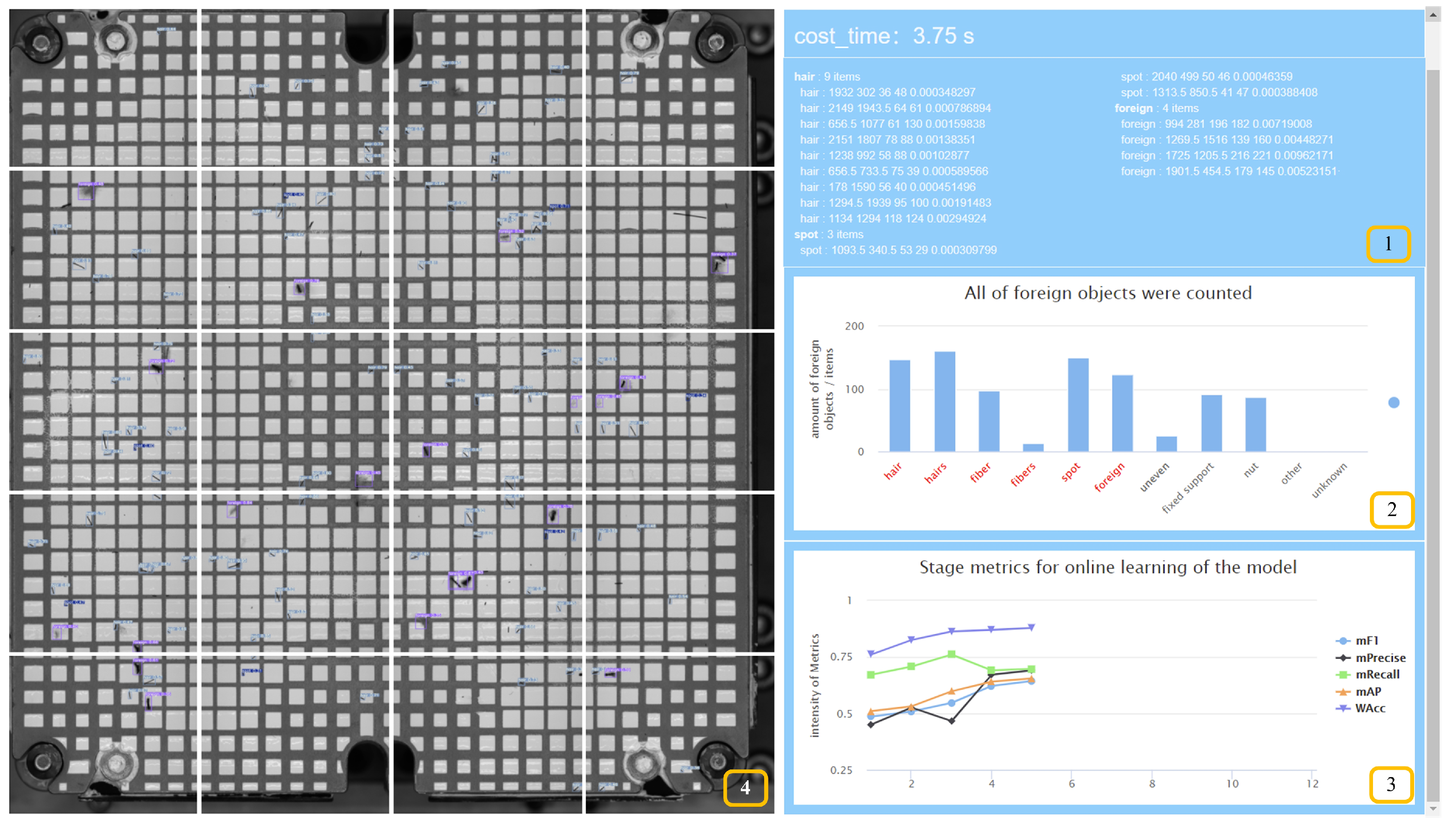
5.2. On-Site Detection
6. Application in Object Detection of Real-World IGBT Coating Operation
7. Conclusions
Author Contributions
Funding
Institutional Review Board Statement
Informed Consent Statement
Data Availability Statement
Conflicts of Interest
Abbreviations
| FGI | Fine-Grained Information |
| WST | Watch and Study Tactic |
| IWS | Information Watch and Study |
| MRD | Mutli-Task Result Discriminant |
| WAcc | WST Accuracy |
Appendix A


Appendix B
Appendix B.1. More Experimental Results

| Model | Acc | mP | mR | mAP | mAP [0.5, 0.95] |
|---|---|---|---|---|---|
| YOLOv7 (baseline) | 91.56% | 73.74% | 68.99% | 54.02% | 33.88% |
| YOLOv7+IWS (ours) | 92.84% | 79.35% | 68% | 57.02% | 35.97% |
| YOLOv7x (baseline) | 91.53% | 69.34% | 70.27% | 53.86% | 33.46% |
| YOLOv7x+IWS (ours) | 92.55% | 69.79% | 69.76% | 58.89% | 37.42% |
Appendix B.2. Ablation Study
| Model | EP | WM | mP | mR | mAP |
|---|---|---|---|---|---|
| YOLOv3 | Y | - | 43.12% | 74.80% | 57.89% |
| Ours | Y | CE | 44.88% | 75.61% | 58.55% |
| P | CE | 45.25% | 75.11% | 58.66% | |
| FGI | Sim | 46.12% | 75.12% | 59.03% | |
| FGI | CE | 46.66% | 76.06% | 59.79% |
Appendix B.3. The Specific Information of IGBT_DF_L Dataset
| IGBT_DF_L | Image | Object | Specific Information (Objects) | ||||||
|---|---|---|---|---|---|---|---|---|---|
| Hair | Hairs | Fiber | Fibers | Spot | Foreign | Uneven | |||
| Train subset | 3544 | 18,139 | 4587 | 233 | 2321 | 467 | 4562 | 5022 | 947 |
| Test subset | 886 | 4512 | 1146 | 145 | 478 | 126 | 1110 | 1274 | 233 |
References
- Zhou, L.Y.; Wang, F. Edge computing and machinery automation application for intelligent manufacturing equipment. Microprocess. Microsyst. 2021, 87, 104389. [Google Scholar] [CrossRef]
- Cusano, C.; Napoletano, P. Visual recognition of aircraft mechanical parts for smart maintenance. Comput. Ind. 2017, 86, 26–33. [Google Scholar] [CrossRef]
- Kang, G.Q.; Gao, S.B.; Yu, L.; Zhang, D.K. Deep Architecture for High-Speed Railway Insulator Surface Defect Detection: Denoising Autoencoder With Multitask Learning. IEEE Trans. Instrum. Meas. 2019, 68, 2679–2690. [Google Scholar] [CrossRef]
- Ge, C.; Wang, J.Y.; Qi, Q.; Sun, H.F.; Liao, J.X. Towards automatic visual inspection: A weakly supervised learning method for industrial applicable object detection. Comput. Ind. 2020, 121, 103232. [Google Scholar] [CrossRef]
- Zuo, D.; Hu, H.; Qian, R.H.; Liu, Z. An insulator defect detection algorithm based on computer vision. In Proceedings of the 2017 IEEE International Conference on Information and Automation (ICIA), Macau, China, 18–20 July 2017; pp. 361–365. [Google Scholar]
- Wang, Y.F.; Wang, Z.P. A survey of recent work on fine-grained image classification techniques. J. Vis. Commun. Image Represent. 2019, 59, 210–214. [Google Scholar] [CrossRef]
- Song, G.; Liu, Y.; Wang, X. Revisiting the Sibling Head in Object Detector. In Proceedings of the 2020 IEEE/CVF Conference on Computer Vision and Pattern Recognition (CVPR), Seattle, WA, USA, 13–19 June 2020. [Google Scholar]
- Behera, A.; Wharton, Z.; Hewage, P.R.P.G.; Bera, A. Context-aware Attentional Pooling (CAP) for Fine-grained Visual Classification. AAAI Conf. Artif. Intell. 2021, 35, 929–937. [Google Scholar]
- He, J.; Chen, J.; Liu, S.; Kortylewski, A.; Yang, C.; Bai, Y.; Wang, C.; Yuille, A. TransFG: A Transformer Architecture for Fine-grained Recognition. In Proceedings of the IEEE/CVF Conference on Computer Vision and Pattern Recognition (CVPR), Nashville, TN, USA, 20–25 June 2021. [Google Scholar]
- Du, R.; Chang, D.; Bhunia, A.K.; Xie, J.; Ma, Z.; Song, Y.Z.; Guo, J. Fine-Grained Visual Classification via Progressive Multi-Granularity Training of Jigsaw Patches. In Proceedings of the European Conference on Computer Vision, Glasgow, UK, 23–28 August 2020. [Google Scholar]
- Tao, H.; Qi, H. See Better Before Looking Closer: Weakly Supervised Data Augmentation Network for Fine-Grained Visual Classification. In Proceedings of the IEEE/CVF Conference on Computer Vision and Pattern Recognition (CVPR), Long Beach, CA, USA, 15–20 June 2019. [Google Scholar]
- Chen, Y.; Bai, Y.L.; Zhang, W.; Mei, T. Destruction and Construction Learning for Fine-Grained Image Recognition. In Proceedings of the IEEE/CVF Conference on Computer Vision and Pattern Recognition (CVPR), Long Beach, CA, USA, 15–20 June 2019; pp. 5152–5161. [Google Scholar]
- Zhou, M.H.; Bai, Y.L.; Zhang, W.; Zhao, T.J.; Mei, T. Look-Into-Object: Self-Supervised Structure Modeling for Object Recognition. In Proceedings of the 2020 IEEE/CVF Conference on Computer Vision and Pattern Recognition (CVPR), Seattle, WA, USA, 13–19 June 2020; pp. 11771–11780. [Google Scholar]
- Schweiker, K.S. Fractal detection algorithm for a LADAR sensor. Proc. SPIE Int. Soc. Opt. Eng. 1993, 1993. [Google Scholar] [CrossRef]
- Lv, F.; Wen, C.; Bao, Z.; Liu, M. Fault diagnosis based on deep learning. In Proceedings of the American Control Conference, Boston, MA, USA, 6–8 July 2016. [Google Scholar]
- Xu, Y.Z.; Yu, G.Z.; Wang, Y.P.; Wu, X.K.; Ma, Y.L. Car Detection from Low-Altitude UAV Imagery with the Faster R-CNN. J. Adv. Transp. 2017, 2017, 1–10. [Google Scholar] [CrossRef] [Green Version]
- Lu, Y.; Yi, S.J.; Zeng, N.Y.; Liu, Y.R.; Zhang, Y. Identification of rice diseases using deep convolutional neural networks. Neurocomputing 2017, 267, 378–384. [Google Scholar] [CrossRef]
- Li, Y.M.; Xu, Y.Y.; Liu, Z.; Hou, H.X.; Zhang, Y.S.; Xin, Y.; Zhao, Y.F.; Cui, L.Z. Robust Detection for Network Intrusion of Industrial IoT Based on Multi-CNN Fusion. Measurement 2019, 154, 107450. [Google Scholar] [CrossRef]
- Jalal, A.; Salman, A.; Mian, A.; Shortis, M.; Shafait, F. Fish detection and species classification in underwater environments using deep learning with temporal information. Ecol. Inform. 2020, 57, 101088. [Google Scholar] [CrossRef]
- Majidifard, H.; Adu-Gyamfi, Y.; Buttlar, W.G. Deep machine learning approach to develop a new asphalt pavement condition index. Constr. Build. Mater. 2020, 247, 118513. [Google Scholar] [CrossRef]
- Zhao, Y.; Yao, Y.; Dong, S.; Zhang, J. Survey on deep learning object detection. J. Image Graph. 2020, 25, 5–30. [Google Scholar]
- Girshick, R. Fast R-CNN. In Proceedings of the IEEE International Conference on Computer Vision, Santiago, Chile, 7–13 December 2015; pp. 1440–1448. [Google Scholar]
- Ren, S.; He, K.; Girshick, R.; Sun, J. Faster R-CNN: Towards Real-Time Object Detection with Region Proposal Networks. IEEE Trans. Pattern Anal. Mach. Intell. 2017, 39, 1137–1149. [Google Scholar] [CrossRef] [Green Version]
- He, K.; Gkioxari, G.; Dollár, P.; Girshick, R. Mask R-CNN. IEEE Trans. Pattern Anal. Mach. Intell. 2017, 42, 2961–2969. [Google Scholar]
- Redmon, J.; Divvala, S.; Girshick, R.; Farhadi, A. You Only Look Once: Unified, Real-Time Object Detection. In Proceedings of the IEEE/CVF Conference on Computer Vision and Pattern Recognition (CVPR), Las Vegas, NV, USA, 27–30 June 2016; pp. 779–788. [Google Scholar]
- Liu, W.; Anguelov, D.; Erhan, D.; Szegedy, C.; Reed, S.; Fu, C.Y.; Berg, A.C. SSD: Single Shot MultiBox Detector. In Proceedings of the European Conference on Computer Vision, Amsterdam, The Netherlands, 11–14 October 2016; pp. 21–37. [Google Scholar]
- Redmon, J.; Farhadi, A. YOLO9000: Better, Faster, Stronger. In Proceedings of the IEEE/CVF Conference on Computer Vision and Pattern Recognition (CVPR), Seattle, WA, USA, 14–19 June 2017; pp. 6517–6525. [Google Scholar]
- Redmon, J.; Farhadi, A. YOLOv3: An Incremental Improvement. arXiv 2018, arXiv:1804.02767. [Google Scholar]
- Bochkovskiy, A.; Wang, C.Y.; Liao, H.Y.M. YOLOv4: Optimal Speed and Accuracy of Object Detection. arXiv 2020, arXiv:2004.10934. [Google Scholar]
- Lin, T.Y.; Goyal, P.; Girshick, R.; He, K.M.; Dollár, P. Focal Loss for Dense Object Detection. IEEE Trans. Pattern Anal. Mach. Intell. 2018, 42, 318–327. [Google Scholar] [CrossRef] [Green Version]
- Lu, X.; Li, B.; Yue, Y.; Li, Q.; Yan, J. Grid R-CNN Plus: Faster and Better. arXiv 2019, arXiv:1906.05688. [Google Scholar]
- Zhang, S.; Chi, C.; Yao, Y.; Lei, Z.; Li, S.Z. Bridging the Gap Between Anchor-based and Anchor-free Detection via Adaptive Training Sample Selection. arXiv 2019, arXiv:1912.02424. [Google Scholar]
- Zhang, M.; Chang, H.; Ma, B.; Wang, N.; Chen, X. Dynamic R-CNN: Towards High Quality Object Detection via Dynamic Training. arXiv 2020, arXiv:2004.06002. [Google Scholar]
- Sun, P.Z.; Zhang, R.F.; Jiang, Y.; Kong, T.; Xu, C.F.; Zhan, W.; Tomizuka, M.; Li, L.; Yuan, Z.H.; Wang, C.H.; et al. Sparse R-CNN: End-to-End Object Detection with Learnable Proposals. In Proceedings of the IEEE/CVF Conference on Computer Vision and Pattern Recognition (CVPR), Nashville, TN, USA, 20–25 June 2021; pp. 14449–14458. [Google Scholar]
- Zhang, H.Y.; Wang, Y.; Dayoub, F.; Sünderhauf, N. VarifocalNet: An IoU-aware Dense Object Detector. In Proceedings of the IEEE/CVF Conference on Computer Vision and Pattern Recognition (CVPR), Nashville, TN, USA, 20–25 June 2021; pp. 8510–8519. [Google Scholar]
- Cai, Z.W.; Vasconcelos, N. Cascade R-CNN: High Quality Object Detection and Instance Segmentation. IEEE Trans. Pattern Anal. Mach. Intell. 2019, 43, 1483–1498. [Google Scholar] [CrossRef] [Green Version]
- Zhang, X.S.; Wan, F.; Liu, C.; Ji, R.R.; Ye, Q.X. FreeAnchor: Learning to Match Anchors for Visual Object Detection. Neural Inf. Process. Syst. 2019, 147–155. [Google Scholar]
- Feng, C.J.; Zhong, Y.J.; Gao, Y.; Scott, M.R.; Huang, W.L. TOOD: Task-aligned One-stage Object Detection. In Proceedings of the IEEE International Conference on Computer Vision, Montreal, BC, Canada, 11–17 October 2021; pp. 3490–3499. [Google Scholar]
- Yun, J.P.; Shin, W.C.; Koo, G.; Kim, M.S.; Lee, C.; Lee, S.J. Automated defect inspection system for metal surfaces based on deep learning and data augmentation. J. Manuf. Syst. 2020, 55, 317–324. [Google Scholar] [CrossRef]
- Chiu, M.C.; Tsai, H.Y.; Chiu, J.E. A novel directional object detection method for piled objects using a hybrid region-based convolutional neural network. Adv. Eng. Inform. 2022, 51, 101448. [Google Scholar] [CrossRef]
- Chen, S.H.; Tsai, C.C. SMD LED chips defect detection using a YOLOv3-dense model. Adv. Eng. Inform. 2021, 47, 101255. [Google Scholar] [CrossRef]
- Zheng, Z.H.; Zhao, J.; Li, Y. Research on Detecting Bearing-Cover Defects Based on Improved YOLOv3. IEEE Access 2021, 9, 10304–10315. [Google Scholar] [CrossRef]
- Duan, L.M.; Yang, K.; Ruan, L. Research on Automatic Recognition of Casting Defects Based on Deep Learning. IEEE Access 2020, 9, 12209–12216. [Google Scholar] [CrossRef]
- Shu, Y.F.; Li, B.; Li, X.M.; Xiong, C.W.; Cao, S.Y.; Wen, X.Y. Deep Learning-based Fast Recognition of Commutator Surface Defects. Measurement 2021, 178, 109324. [Google Scholar] [CrossRef]
- Yao, J.H.; Li, J.F. AYOLOv3-Tiny: An improved convolutional neural network architecture for real-time defect detection of PAD light guide plates. Comput. Ind. 2021, 136, 103588. [Google Scholar] [CrossRef]
- Zhang, T.J.; Zhang, C.R.; Wang, Y.J.; Zou, X.F.; Hu, T.L. A vision-based fusion method for defect detection of milling cutter spiral cutting edge-ScienceDirect. Measurement 2021, 177, 109248. [Google Scholar] [CrossRef]
- Zhu, J.S.; Li, X.T.; Zhang, C. Fine-grained identification of vehicle loads on bridges based on computer vision. J. Civ. Struct. Health Monit. 2022, 177, 427–446. [Google Scholar] [CrossRef]
- Araujo, V.M.; Britto, A.S.; Oliveira, L.S.; Koerich, A.L. Two-View Fine-grained Classification of Plant Species. Neurocomputing 2021, 467, 427–441. [Google Scholar] [CrossRef]
- Zhao, Q.; Wang, X.; Lyu, S.C.; Liu, B.H.; Yang, Y.F. A Feature Consistency Driven Attention Erasing Network for Fine-Grained Image Retrieval. Pattern Recognit. 2022, 128, 108618. [Google Scholar] [CrossRef]
- Behera, A.; Wharton, Z.; Liu, Y.; Ghahremani, M.; Bessis, N. Regional Attention Network (RAN) for Head Pose and Fine-grained Gesture Recognition. IEEE Trans. Affect. Comput. 2020, 14, 1949–3045. [Google Scholar] [CrossRef]
- Chen, T.; Kornblith, S.; Norouzi, M.; Hinton, G. A Simple Framework for Contrastive Learning of Visual Representations. In Proceedings of the 25th Americas Conference on Information Systems, Cancún, Mexico, 15–17 August 2019. [Google Scholar]
- Rostianingsih, S.; Setiawan, A.; Halim, C.I. COCO (Creating Common Object in Context) Dataset for Chemistry Apparatus. Procedia Comput. Sci. 2020, 171, 2445–2452. [Google Scholar] [CrossRef]
- Hülsmann, A.; Zech, C.; Klenner, M.; Tessmann, A.; Leuther, A.; Lopez-Diaz, D.; Schlechtweg, M.; Ambacher, O. Radar System Components to Detect Small and Fast Objects. Int. Soc. Opt. Photonics 2015, 9483, 94830C. [Google Scholar]
- Kisantal, M.; Wojna, Z.; Murawski, J.; Naruniec, J.; Cho, K. Augmentation for small object detection. In Proceedings of the 9th International Conference on Advances in Computing and Information Technology, Bangalore, India, 27 December 2019. [Google Scholar]


| Data Set | At | Lt | Mt | St |
|---|---|---|---|---|
| MS-COCO | 3.5–7.7 | 25% | 34% | 41% |
| IGBT_DF (ours) | 4–8 | 27% | 27% | 46% |
| IGBT_DF | Image | Object | Specific Information (Objects) | ||||||
|---|---|---|---|---|---|---|---|---|---|
| Hair | Hairs | Fiber | Fibers | Spot | Foreign | Uneven | |||
| Train subset | 717 | 3018 | 739 | 58 | 395 | 84 | 722 | 883 | 137 |
| Test subset | 180 | 840 | 253 | 14 | 102 | 22 | 152 | 256 | 41 |
| Positive | Negative | |
|---|---|---|
| True | Tp | Tn |
| False | Fp | Fn |
| Model | Backbone | Acc | mAP | mR | mP | FPS |
|---|---|---|---|---|---|---|
| Faster R-CNN | Resnet-50 | 90.69% | 39.11% | 43.92% | 49.39% | 21.4 |
| Resnet-101 | 90.74% | 35.86% | 42.38% | 50.71% | 15.6 | |
| RetinaNet | Resnet-101 | 89.23% | 24.28% | 62.97% | 4.93% | 15 |
| Cascade R-CNN | Resnet-50 | 89.66% | 39.17% | 50.71% | 50.59% | 16.1 |
| Resnet-101 | 90.09% | 39.44% | 55.11% | 37.67% | 13.5 | |
| Grid R-CNN | Resnet-50 | 90.75% | 38.47% | 50.11% | 19.49% | 15 |
| Resnet-101 | 91.27% | 37.15% | 50.35% | 27.44% | 12.6 | |
| Resnext-101 | 91.33% | 38.42% | 50.36% | 30.59% | 10.8 | |
| FreeAnchor | Resnet-50 | 91.34% | 34.77% | 75.11% | 4.81% | 18.4 |
| ATSS | Resnet-50 | 90.92% | 48.50% | 76.90% | 7.46% | 19.7 |
| Resnet-101 | 91.26% | 43.14% | 76.42% | 8.07% | 12.3 | |
| Resnext-101 | 91.34% | 43.7% | 76.41% | 6.58% | 11 | |
| Dynamic R-CNN | Resnet-50 | 89.59% | 40.84% | 49.40% | 44.24% | 18.2 |
| Sparse R-CNN | Resnet-50 | 89.33% | 35.12% | 82.26% | 3.83% | 22.5 |
| Resnet-101 | 89.86% | 38.93% | 76.66% | 3.57% | 18.5 | |
| Resnext-101 | 89.92% | 39.37% | 80.92% | 3.91% | 17 | |
| TOOD | Resnet-50 | 90.04% | 47.05% | 76.90% | 15.83% | 19.3 |
| Resnet-101 | 90.53% | 44.40% | 78.69% | 9.66% | 18.1 | |
| Resnext-101 | 90.12% | 47.67% | 78.96% | 10.21% | 17 | |
| VarifocalNet | Resnet-50 | 90.67% | 47.01% | 77.97% | 7.49% | 19.3 |
| Resnet-101 | 90.56% | 47.24% | 75.47% | 6.84% | 15.6 | |
| Resnext-101 | 90.51% | 47.67% | 75.66% | 7.29% | 14 | |
| YOLOv3 | Darknet-53 | 89.86% | 50.98% | 67.18% | 45.16% | 35 |
| YOLOv3+IWS (ours) | Darknet-53 | 91.48% | 53.12% | 70.73% | 52.58% | 34 |
| IGBT_DF_L | Train Images | Test Images | Train Objects | Test Objects |
|---|---|---|---|---|
| 3544 | 886 | 18,139 | 4512 |
| Model | FRC | RN | CRC | GRC | FA | |||||
| R-50 | R-101 | R-101 | R-50 | R-101 | R-50 | R-101 | Rx-101 | R-50 | R-101 | |
| mAP | 44.09% | 43.71% | 43.25% | 45.09% | 44.98% | 42.82% | 42.70% | 43.17% | 52.50% | 52.31% |
| Model | ATSS | DRC | SRC | TOOD | ||||||
| R-50 | R-101 | Rx-101 | R-50 | R-50 | R-101 | Rx-101 | R-50 | R-101 | Rx-101 | |
| mAP | 52.80% | 52.10% | 52.34% | 45.12% | 44.84% | 53.33% | 54.11% | 54.01% | 52.15% | 53.17% |
| Model | VN | Y3 | Y3-T | |||||||
| R-50 | R-101 | Rx-101 | D53 | D53 | ||||||
| mAP | 54.04% | 52.85% | 53.6% | 57.89% | 59.79% | |||||
| Model | Acc | mP | mR | mAP | mAP [0.5, 0.95] | WAcc | FPS |
|---|---|---|---|---|---|---|---|
| YOLOv3 (baseline) | 89.86% | 45.16% | 67.18% | 50.98% | - | 76.13% | 35 |
| YOLOv3+IWS (ours) | 91.48% (+1.62%) | 52.58% (+7.42%) | 70.73% (+2.55%) | 53.12% (+2.14%) | - | 82.52% (+6.39%) | 34 |
| YOLOv3-spp (baseline) | 90.07% | 46.24% | 56.60% | 50.11% | - | 75.86% | 20 |
| YOLOv3-spp+IWS (ours) | 91.55% (+1.48%) | 46.08% (−0.16%) | 69.48% (+12.88%) | 53.46% (+3.35%) | - | 82.40% (+6.54%) | 31 |
| YOLOv5l (baseline) | 90.85% | 76.13% | 63.73% | 53.69% | 32.36% | - | 140 |
| YOLOv5l-op (ours) | 90.33% (−0.52%) | 79.89% (+3.76%) | 62.3% (−1.43%) | 54.67% (+0.98%) | 32.43% (+0.07%) | - | 132 |
| YOLOv5l+IWS (ours) | 91.71% (+1.37%) | 77.7% (+1.57%) | 65.1% (+1.37%) | 56.79% (+3.1%) | 35.23% (+2.87%) | - | 126 |
| Model | Acc | mP | mR | mAP | mAP [0.5, 0.95] | WAcc | FPS |
|---|---|---|---|---|---|---|---|
| YOLOv3 (baseline) | 91.71% | 43.12% | 74.8% | 57.89% | - | 84.72% | 35 |
| YOLOv3+IWS (ours) | 92.89% (+1.28%) | 46.66% (+3.54%) | 76.06% (+1.26%) | 59.79% (+1.9%) | - | 86.34% (+1.62%) | 34 |
| YOLOv3-spp (baseline) | 92.08% | 44.53% | 75.49% | 59.28% | - | 84.98% | 20 |
| YOLOv3-spp+IWS (ours) | 93.10% (+1.02%) | 45.02% (+0.49%) | 75.85% (+0.36%) | 59.45% (+0.17%) | - | 87.01% (+2.03%) | 31 |
| YOLOv5l (baseline) | 93.63% | 68.24% | 67.18% | 64.09% | 42.66% | - | 140 |
| YOLOv5l-op (ours) | 93.66% (+0.03%) | 67.17% (−1.07%) | 69.04% (+1.86%) | 64.08% (−0.1%) | 43.61% (+0.95%) | - | 132 |
| YOLOv5l+IWS (ours) | 93.89% (+0.26%) | 69.07% (+0.83%) | 69.76% (+2.58%) | 65.49% (+1.4%) | 44.46% (+1.8%) | - | 126 |
Publisher’s Note: MDPI stays neutral with regard to jurisdictional claims in published maps and institutional affiliations. |
© 2022 by the authors. Licensee MDPI, Basel, Switzerland. This article is an open access article distributed under the terms and conditions of the Creative Commons Attribution (CC BY) license (https://creativecommons.org/licenses/by/4.0/).
Share and Cite
Huang, H.; Luo, X. A Holistic Approach to IGBT Board Surface Fractal Object Detection Based on the Multi-Head Model. Machines 2022, 10, 713. https://doi.org/10.3390/machines10080713
Huang H, Luo X. A Holistic Approach to IGBT Board Surface Fractal Object Detection Based on the Multi-Head Model. Machines. 2022; 10(8):713. https://doi.org/10.3390/machines10080713
Chicago/Turabian StyleHuang, Haoran, and Xiaochuan Luo. 2022. "A Holistic Approach to IGBT Board Surface Fractal Object Detection Based on the Multi-Head Model" Machines 10, no. 8: 713. https://doi.org/10.3390/machines10080713