1. Introduction
Maglev trains have the advantages of low noise and good ride comfort, and are suitable for use in urban environments [
1,
2,
3,
4]. To date, maglev trains have made great progress, and have been commercialized in Shanghai, Hunan and other places in China.
However, during the development of these maglev train systems, vehicle–guideway coupled vibration has been encountered, and this seems to be a factor that hinders the maglev guideway from decreasing its weight and cost. Most researchers believe that low track stiffness is an important cause of vehicle–guideway coupled vibration; the lower the linear density of the track beam, the worse the stability of the suspension system, and the more likely the vehicle–guideway coupled vibration will occur over time [
5,
6]. However, the higher the track stiffness requirement, the higher the track construction cost. Track construction costs account for about 60–70% of the overall construction cost of the maglev system [
7,
8], so strong tracks will significantly increase their overall construction cost. The occurrence of this problem is also related to the characteristics of the maglev train suspension system. Maglev trains rely on controlled electromagnetic force to levitate, which makes the suspension control system key to the stable operation of maglev trains. However, while the electromagnetic force acts on the vehicle, it also brings an energy input to the track, which has an impact on the deformation of the guideway, which, in turn, causes the levitation controller to adjust the electromagnetic force. In the case of low track stiffness, the track may vibrate severely under the action of electromagnetic force when the control algorithm is not perfect, which may even cause serious problems such as the electromagnet hitting the track. This problem has been encountered in many cases [
9,
10,
11]. Sun et al., analyzed the causes of maglev vehicle–guideway coupling vibration by connecting Hopf bifurcation with vehicle–guideway coupling vibration, and noted that the time delay inside the system directly led to the generation of coupling vibration [
12]. Wang et al., analyzed the mechanism of coupled vibration in detail from multiple angles, deduced the frequency range of self-excited vibration, and analyzed the factors affecting the stability of the coupled system [
13]. Li et al., noted that the eigenfrequency of the coupled vibration was close to the natural frequency of the rail beam, so it would be effective to the eigenfrequency of the coupled system away from the natural frequency of the beam [
14]. Liang et al., also studied the vibration characteristics of the vehicle at different speeds through experiments, and noted the range of the vibration frequency of the track beam and the influence of the vehicle speed, on the vibration characteristics [
15].
Many researchers have tried to solve the vehicle–guideway coupled vibration problem from the perspective of control algorithm design. In [
16], the influence of different signals on feedback control was studied, and it was found that using the gap signal directly in the displacement sensor increased the possibility of coupled vibration problems, while the gap signal, considering the state of the track beam, could effectively suppress the vibration. In [
17], the mathematical model of the five-point suspension vehicle–guideway coupling system based on electromagnetic force control was established, the influence of the controller parameters on the vibration was analyzed, and a method to suppress the vibration by adjusting the controller parameters was found. Some researchers have also tried to solve this problem from the perspective of the mechanical structure of the maglev system. Zhang et al., presented a scheme to suppress the coupled vibration of the vehicle–guideway through the use of air springs [
8].
High stiffness rails will result in higher construction costs. Therefore, the question of how to achieve suspension control of maglev trains under the condition of low track stiffness has become key to reducing the construction cost of maglev trains, and also key to promoting their commercial application. In [
18], the suspension control strategy of a maglev train using flexible track was studied, and a sliding mode control algorithm based on RBF network approximation was designed, which had good anti-interference ability.
A series of control schemes rely on electromagnetic force feedback control, and in these control schemes, an accurate electromagnetic force estimation method is needed. In [
19], an empirical nonlinear formula based on the magnetic circuit calculation method was given. This model ignored the leakage flux and reluctance of the electromagnet core and guideway, and was widely used by many researchers. However, this model ignored the influence of leakage flux, and the error was large when the position was far from the equilibrium point. In [
20], a more complex but accurate electromagnetic force calculation method considering the track state was given, but the model was slightly complicated, and was difficult to apply to real-time levitation control. In [
21], levitation force characteristics were deeply studied by finite element analysis, an accurate electromagnetic force model was proposed, and the control algorithm using this model was validated by experiments to show an effective improvement in control performance.
Due to the highly nonlinear characteristics of the magnetic suspension system, the conventional linearization method generates a large error, which further increases the error of the controller, and increases the difficulty of control. Considering that feedback linearization can accurately achieve the linearization of nonlinear systems, this method is often used in suspension control. In [
22], a sliding mode control method based on feedback linearization was studied, which showed a good robustness. In [
23], the coupled model was decoupled, and a controller was designed based on the theory of feedback linearization, which achieved decoupling between the front and rear suspension points in the same levitation module, thus, the vibration caused by coupling between the two points in the presence of track irregularity was greatly suppressed.
In this paper, the system model of the suspension system including the guideway state, was first established, and then, a simple but more accurate electromagnetic force model was established based on the least squares fitting method. On this basis, the feedback linearization method was used to establish an accurate linearized model of the suspension system, and then a controller was designed to suppress the coupled vibration under low track stiffness. Experiments were carried out to validate the proposed electromagnetic force model. Experiments on an suspension experimental platform with low guideway stiffness further proved that the control algorithm proposed in this paper had excellent control effect, achieved suspension control under low guideway stiffness, and had strong anti-interference ability.
2. Modeling of the Maglev Vehicle–Guideway Coupled System
In order to better study the problem of vehicle–guideway coupling vibration, the selection of the research object was very important. As the actual maglev train system is relatively complex, it is difficult to study the complete system. Therefore, the minimum coupling element of the vehicle–guideway coupling system was selected as the research object of this paper. It has previously been proven that the flexible guideway can be deemed as a series of mass–spring–damper systems, and the maglev vehicle–guideway coupled system can be simplified to being a single electromagnet suspension control system and a mass-spring-damper system, if only one vibration mode of the guideway is concerned. At the same time, we noted that the coupled vibration of the vehicle–guideway occurs mainly in the vertical direction, so its motion in other directions was ignored in this paper. The track beam was regarded as a Bernoulli–Eulerian beam, to further simplify the system.
2.1. Modeling of the Magnetic Suspension System
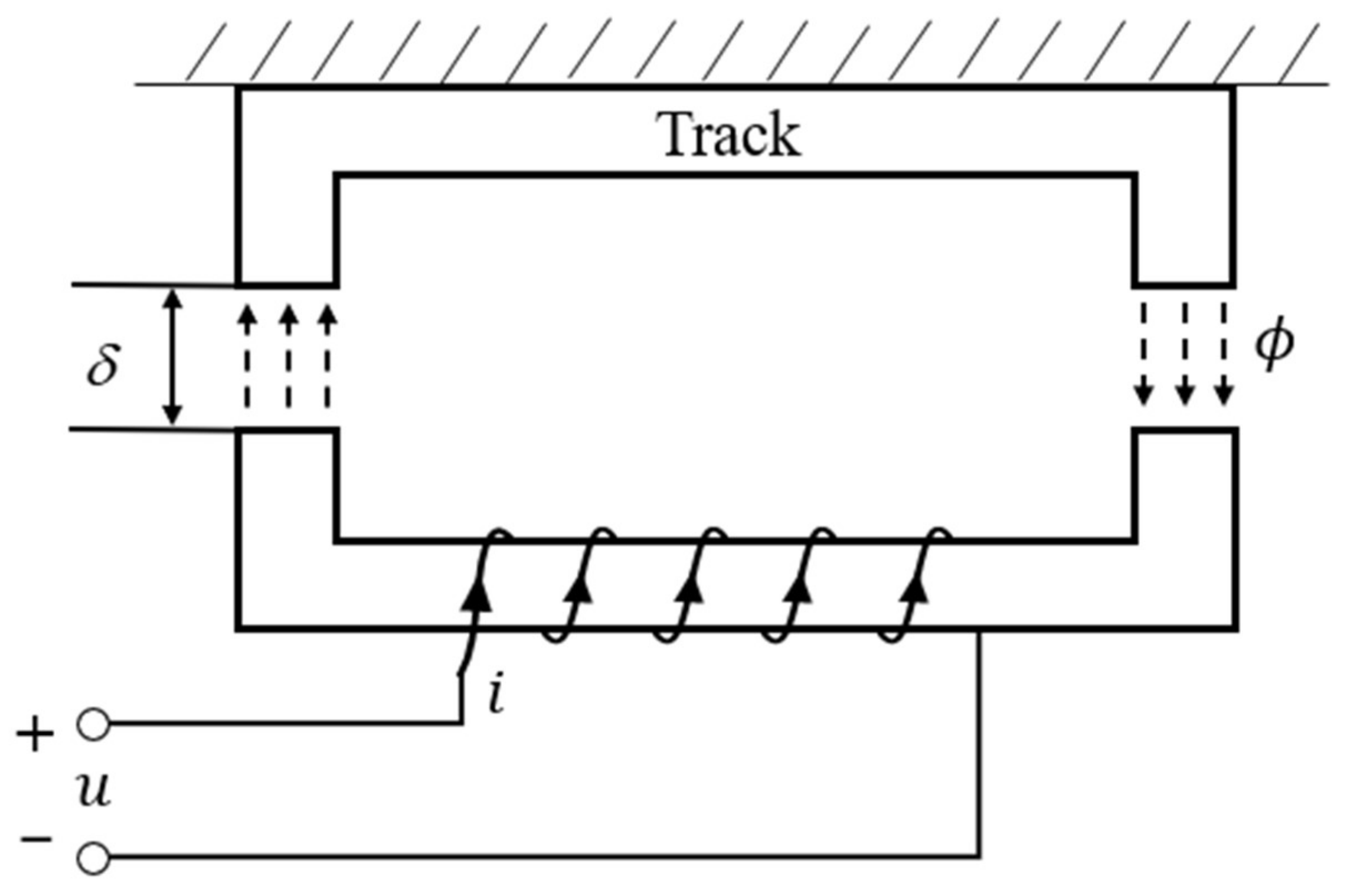
The simplified single-point suspension structure is shown in
Figure 1. Here,
δ is the air gap between the suspension electromagnet and the track, and
ϕ is the air gap magnetic flux. Suppose
u is the voltage applied to the electromagnet winding,
B is the magnetic flux density in the air gap, and
i is the current through the winding. The remaining parameters used in the modeling process are as follows:
m1 is the mass of the suspension electromagnet,
F is the electromagnetic force between the electromagnet and the track,
N is the number of turns of the electromagnet,
S is the pole area of the electromagnet,
μ0 is the vacuum permeability,
W is the work performed by the electromagnetic force on the electromagnet, R is the resistance on the winding,
Fm is the magneto-motive force,
Rm is the electromagnet reluctance, and
g is the gravitational acceleration. The vertical downward direction was selected as the positive direction.
Firstly, it is supposed that the track is fixed, thus, the dynamic equation of the electromagnet is given by:
If the magnetic flux leakage between the air gap is ignored, the electromagnetic force can be obtained by:
Here we observe the commonly used electromagnetic force model ignoring the magnetic flux leakage, which can estimate the electromagnetic force within a certain gap range. It can be seen that the electromagnetic force is proportional to the square of the magnetic flux density in this electromagnetic force model.
The voltage balance equation of the electromagnet can be given by [
24]:
Ignoring the leakage magnetic flux, the magnetic flux across the electromagnet air gap can be obtained:
Therefore, the magnetic flux density is:
Substituting Equation (5) into Equation (3) yields:
Combining the above equations together, the mathematical model of the suspension system is obtained:
2.2. Modeling of the Maglev Track
The elevated guideway is frequently used in the maglev system. Many research papers have shown that the vehicle–guideway coupled vibration is closely related to the elasticity of the track beam.
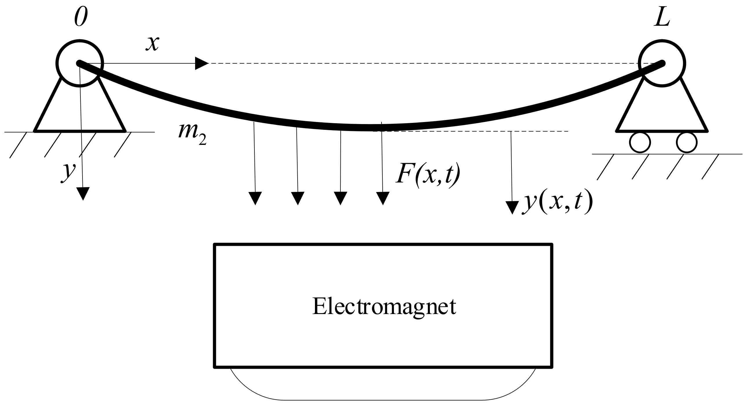
Since the dimensions of the maglev girder cross-section are far smaller than the length of the girder, the track beam is simplified as a flexible Bernoulli–Euler beam.
Figure 2 shows the simplified model of the vehicle–guideway coupled system.
F is the electromagnetic force acting on the track beam, and
L and
m2 are the length and mass of the track beam, respectively. Only the vertical motion of the track is considered, and the motion equation of the track is given by:
Here, EI is the bending stiffness of track beam, and is the linear mass of the track beam.
The displacement of the beam can be described as the combined motions of a series of specified beam modes:
Here,
is the
i-th order normalized modal function of the track beam, and
is the
i-th order generalized time-domain coordinates of the track beam. For a simply supported beam, the modal frequencies and modal functions of the
i-th vibration mode are:
Substitute Equation (11) into Equation (9), multiply both sides of the equation by
, then integrate along the track beam from 0 to
L, and use the orthogonality condition of the beam to obtain:
Here,
is the generalized force of the
i-th mode, and:
Taking the first-order mode of the track into account as an example, Equation (13) can be simplified as:
Taking the states of the track beam as a part of the system states, the complete mathematical model of the system becomes:
3. Electromagnetic Force Model Based on Least Squares Fitting
The electromagnetic force model ignoring the magnetic flux leakage was given in Equation (2). However, leakage flux cannot be avoided in the practical magnetic levitation system, and the flux exists in the nearby space instead of only in the air gap between the polar areas of the electromagnet and the track, which causes the traditional empirical formula to contain a certain error. Subsequent experiments also confirm the existence of this error.
In order to find a more accurate electromagnetic force model to provide a more accurate reference for electromagnetic force feedback, the current empirical model was revised by a combination of measured data and least squares fitting. The data, including the current through the electromagnet and the suspension gap, was obtained on a magnetic suspension experimental platform at a different suspension heights.
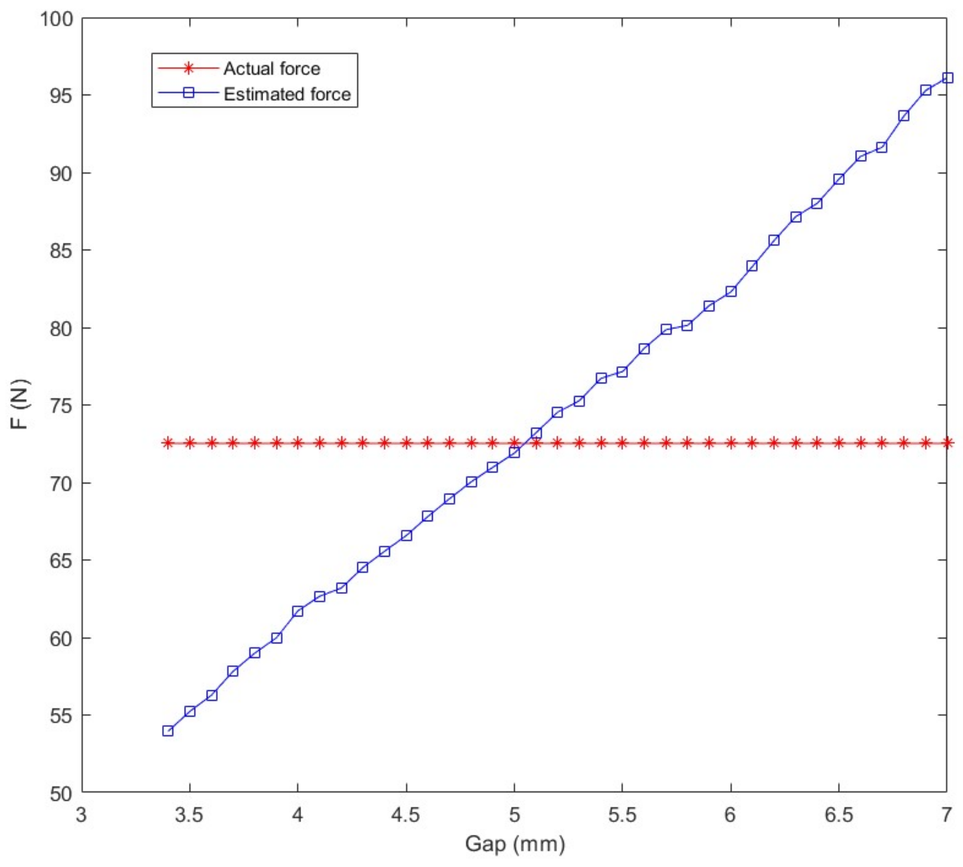
Table 1 gives the relevant parameters of the experimental platform.
Figure 3 shows the electromagnetic forces obtained from the experiments, and as a comparison, the electromagnetic forces estimated by the empirical formula are also plotted in the same figure. It can clearly be seen that there were obvious errors between the electromagnetic forces estimated by the empirical formula, and the real electromagnetic forces; the estimated electromagnetic force increased significantly as the gap increased, while the actual electromagnetic force remained the same (which equaled the weight of the suspension load). In this section of the paper, several possible LS fit formulas are proposed, to find the best electromagnetic force estimation model.
3.1. Introduction of Suspension Gap into Empirical Formula
Affected by the leakage magnetic flux, the electromagnetic force will always be affected by the suspension gap, so the suspension gap was introduced into the model. The two most common function models were adopted, which not only increases the electromagnetic force with the decrease in the suspension gap, but also could be implemented into the control system relatively simply. Let:
Then, the optimal value of
k can be obtained:
Substituting Equation (17) into Equation (18), then
k = 0.077141 is obtained.
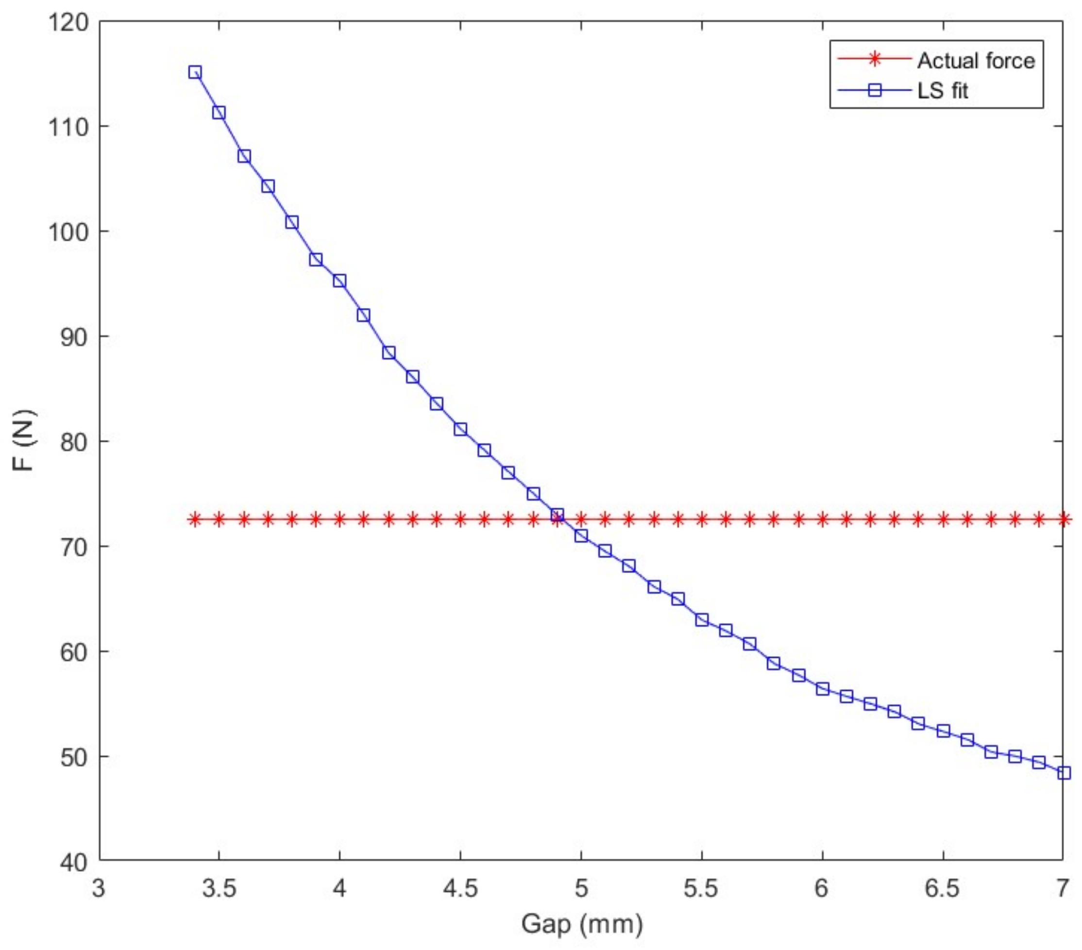
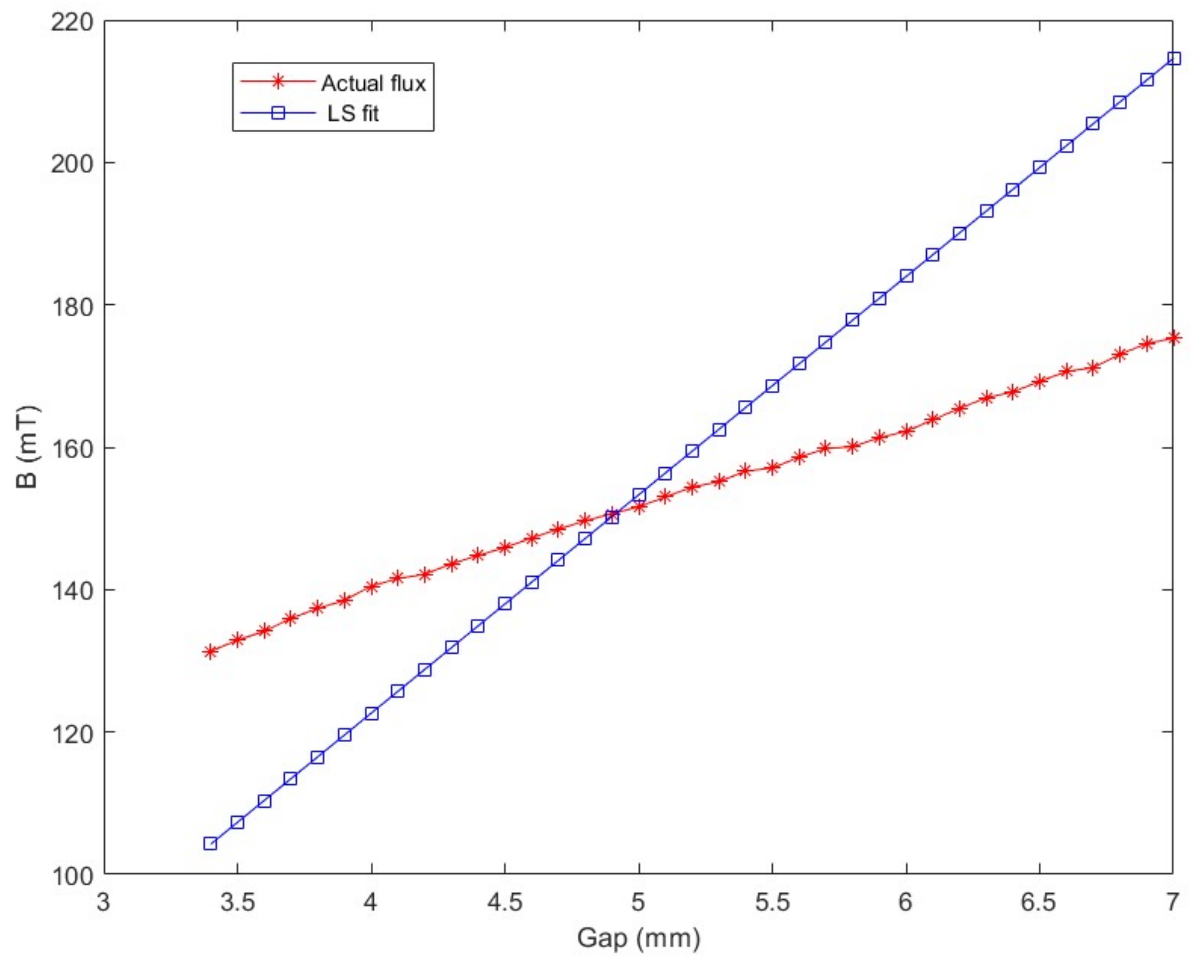
Figure 4 shows the relationship between the electromagnetic force estimated by the LF fit, the actual electromagnetic force and the suspension gap. When the suspension gap was 3.5 mm, the electromagnetic force error reached 58.76%, which was much larger than the empirical formula. It can be seen that the fitting formula was far from meeting the requirements for accuracy, and a comparison between calculated results of the magnetic fluxes given in
Figure 5, and the actual values, also supports this conclusion. Note that after the introduction of
δ2, the estimated value of the electromagnetic force changed from an increase with the increase in the gap, to a decrease with the increase in the gap; that is to say, the contribution of
δ to the electromagnetic force was a little too large at this time. Therefore, a new fitting model was proposed.
Substituting Equation (20) into Equation (18), then
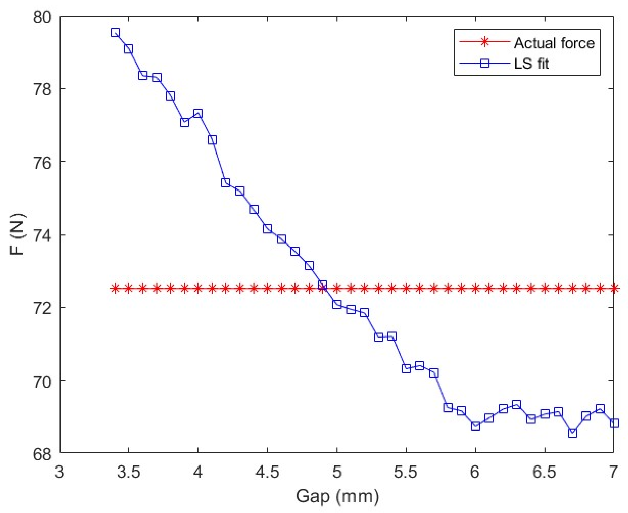
k = 15.672928 is obtained. The fitting result of the electromagnetic force is shown in
Figure 6. The error, this time, was reduced to 9.67%, which is obviously better than the previous two models. At this time, the introduction of
δ−1 compensated for the electromagnetic force under the small gap, reduced the electromagnetic force under the large gap, and improved the problems existing in the empirical formula, but the compensation under the small gap was still too large.
Figure 7 shows the relationship between the estimated magnetic flux and the actual magnetic flux; it can be seen that the estimated magnetic flux, this time, was very close to the real value.
3.2. The Final Model
Considering that the data obtained by Equation (19) were close to the experimental data, the estimated electromagnetic force was just a little too strong under small gaps. While a small change in
δ can cause a huge change in
δ−1 when the gap is close to 0, it can be understood that the estimated electromagnetic force produces a large error under small gaps. In order to avoid this problem, the term (
δ +
k2)
−1 was used to replace
δ−1 so that the problem of the parameter changing too dramatically at small gaps could be avoided. Assuming that:
Then, it can be rewritten as:
Then, substituting Equations (23) and (24) into Equation (22) yields:
Then, the matrix form of Equation (22) is obtained. The experimental data are substituted into Equation (18), and
θ = [0.0501126, 6.803929 × 10
−5] is obtained, that is,
k1 = 19.955073,
k2 = 0.00135773. In order to verify the fitting effect,
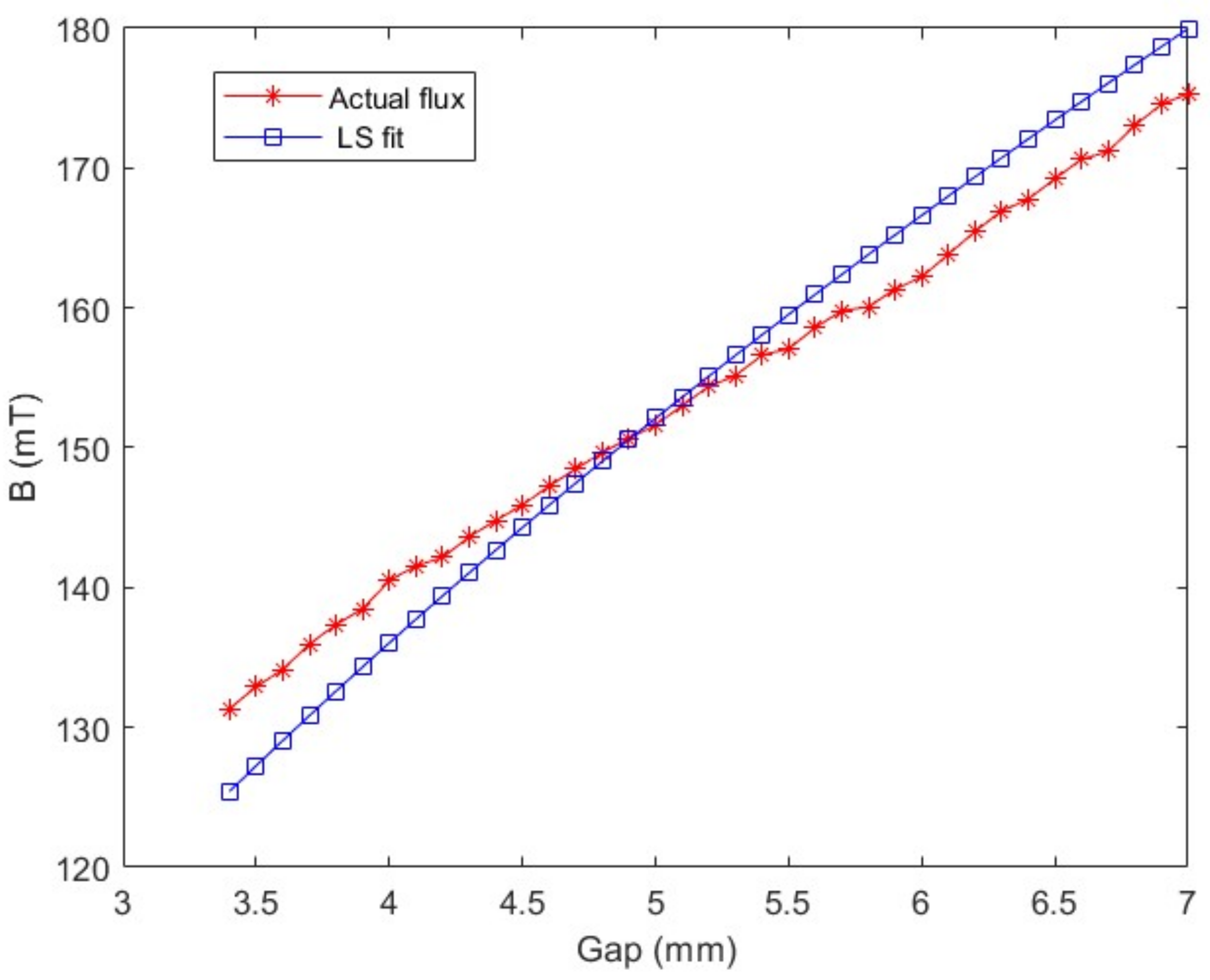
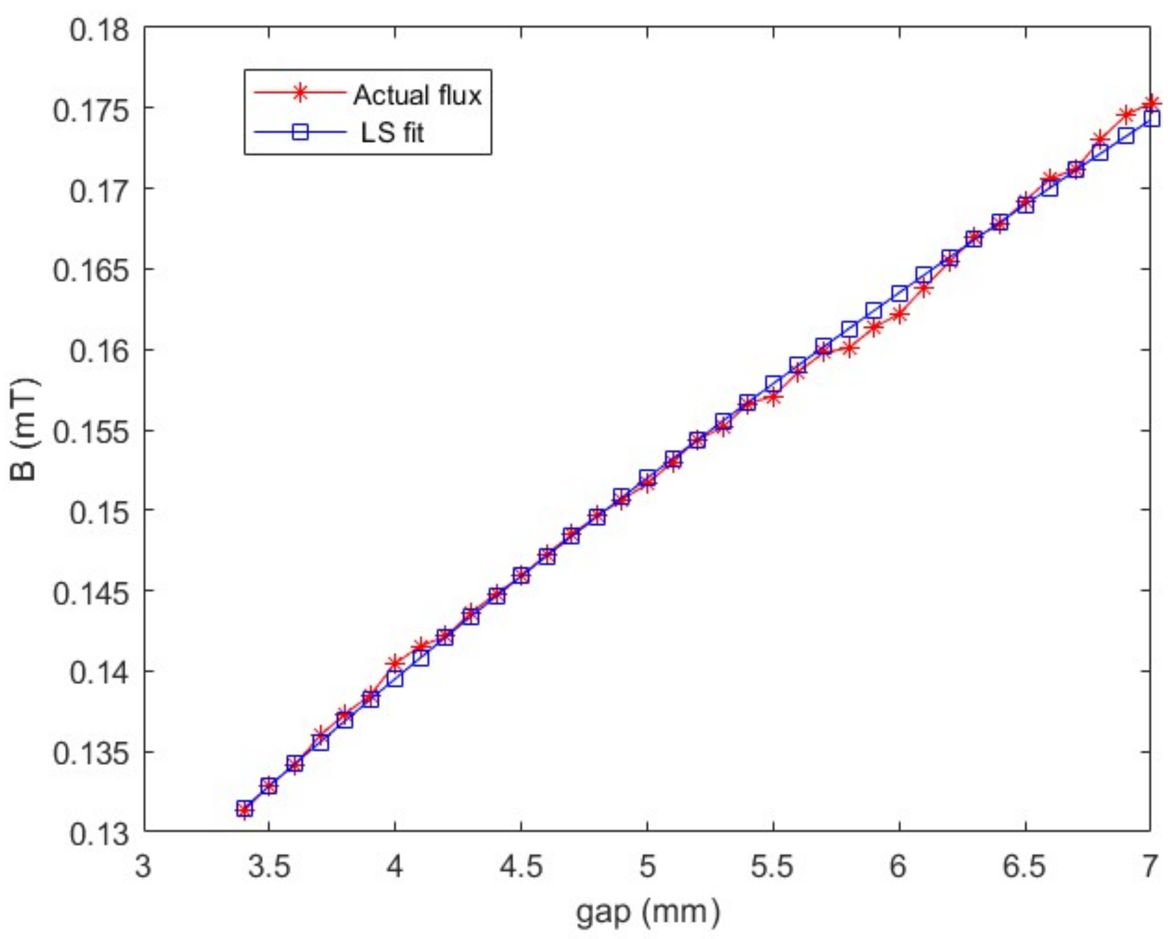
Figure 8 shows the comparison between the estimated value and the actual value of the electromagnetic forces at different suspension gaps. It can clearly be seen that the estimated value of the electromagnetic force was very close to the real value, the maximum error was only 1.59%, and the accuracy of the model met the requirements.
Figure 9 shows the estimated magnetic flux and the measured magnetic flux, in which it can be seen that the estimated value was basically the same as the actual value.
Substituting Equation (21) into Equation (15), a new system model is obtained:
4. Design of Feedback Linearization Controller to Suppress the Coupled Vibration
The model of the suspension system given in
Section 2 was highly nonlinear. Many of the levitation controllers proposed in previous literature were designed based on the linearized dynamic model; however, as the levitation gap moves away from the equilibrium position, the error between the linearized model and the real system becomes more prominent, which has a certain impact on the performance of the controller. To avoid this effect, we used the feedback linearization technique to obtain an equivalent linearized system model.
4.1. Feedback Linearization of the Suspension System
Equation (15) describes the model of the suspension system, which is a fourth order system. Define:
Then, the state space equation of the system is obtained:
and define:
Equation (28) can be rewritten as:
For the function f and h that is smooth over the domain
, its Lie derivative is:
and
. It can be seen that for the current system there are:
It is guaranteed that
LgLfh(
x) = 0, and the relative order of the system is four, which indicates that the system is able to accurately feedback linearization. Then, substituting Equation (34) into the Lie derivatives of the various orders of the system, yields:
Let
u =
α(
x) +
β(
x)
v, where:
While the homeomorphic mapping of the system is:
The linearized system model is obtained as:
The equilibrium point of the system is
, that is:
, where
and
are the expected values of
and
, respectively. Then, state feedback control is used:
Then, the transfer function of the system can be obtained as:
In order to ensure that the closed-loop poles of the system are on the left side of the imaginary axis, we can obtain from the Rouse criterion:
Therefore, the stability of the system can be guaranteed when the feedback gains satisfy Equation (45). Considering that the electromagnetic force should be slightly larger than the gravity during the suspension process, this means the expected value of the electromagnetic force
, namely:
which means that the gain of the transfer function must be small enough. Then from Equation (29), the expected input magnetic flux of
B can be obtained as:
from which the system control law based on magnetic flux feedback is obtained.
However, considering that the actual suspension system is controlled by voltage, it is necessary to convert the control signal from a magnetic flux signal to a voltage signal.
4.2. Design of the Magnetic Flux Loop
The magnetic flux signal cannot be directly applied to the real system. In fact, the change of the magnetic flux signal is achieved by adjusting the input voltage.
The relationship of magnetic flux and voltage can be obtained by Equation (6):
It can be seen that the magnetic flux varies with the voltage and the suspension gap, so the suspension gap should also be taken into account in the design of the magnetic flux loop.
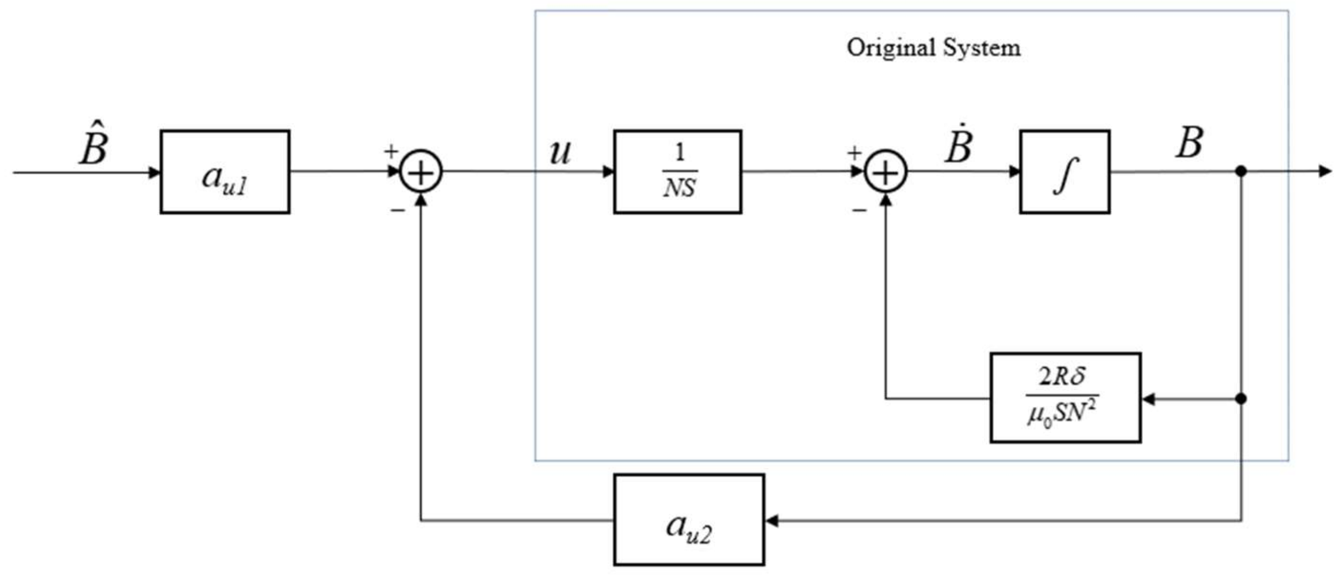
Figure 10 shows the structure of the magnetic flux loop, in which the part inside the block is the original physical system. Define:
were
and
are feedback control gains. Substituting Equation (49) into Equation (48), yields:
The goal is to impel the flux in the air gap to follow the desired flux as quickly as possible with as little error as possible. When
, it is expected that
. Note the gain of
is related to
in Equation (50), so it is necessary to make
and
, be related to
. Let:
where
is a positive real constant. Substituting Equation (51) into Equation (50) yields:
Now
when
is satisfied. Then, substituting Equations (47) and (51) into Equation (49) yields:
which is the control law.
4.3. Estimation of the Track State
The displacement and speed of the track cannot be directly obtained in the actual maglev system, which means that the states of the track, and , could not be directly obtained. The commonly measurable quantities are the states of the vehicle, such as the vertical acceleration of the electromagnet, , the levitation gap, , and the magnetic flux density of the gap, . Therefore, it is necessary to estimate the track states using the measurable states.
Note that the absolute acceleration of the electromagnet is:
Therefore,
can be obtained:
can be obtained by integration of
:
Now all the states have been obtained, and the control algorithm can be applied to the real maglev system.
5. Experimental Verification
In order to verify the control effect of the algorithm proposed above, the control algorithm was tested on a vehicle–guideway coupled vibration experimental platform.
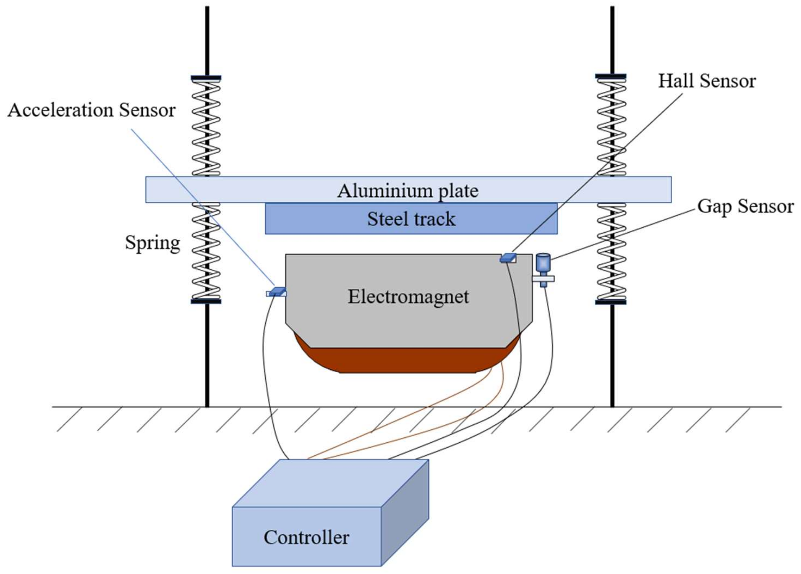
Figure 11 shows the structure diagram of the experimental platform, which consisted of a suspension electromagnet, a suspension track, sensors, support rods, support springs, control boxes, and a power supply, etc. The support rod was fixed in the vertical direction, and the upper and lower springs were fixed along the support rods, supporting the aluminum plate and the guideway. There was a groove at the upper surface of the iron core of the electromagnet, and a Hall sensor was placed in this groove to measure the magnetic flux density in the air gap; a gap sensor and an accelerometer were also fixed on the electromagnet. Some relevant parameters of the experimental platform are given in
Table 2.
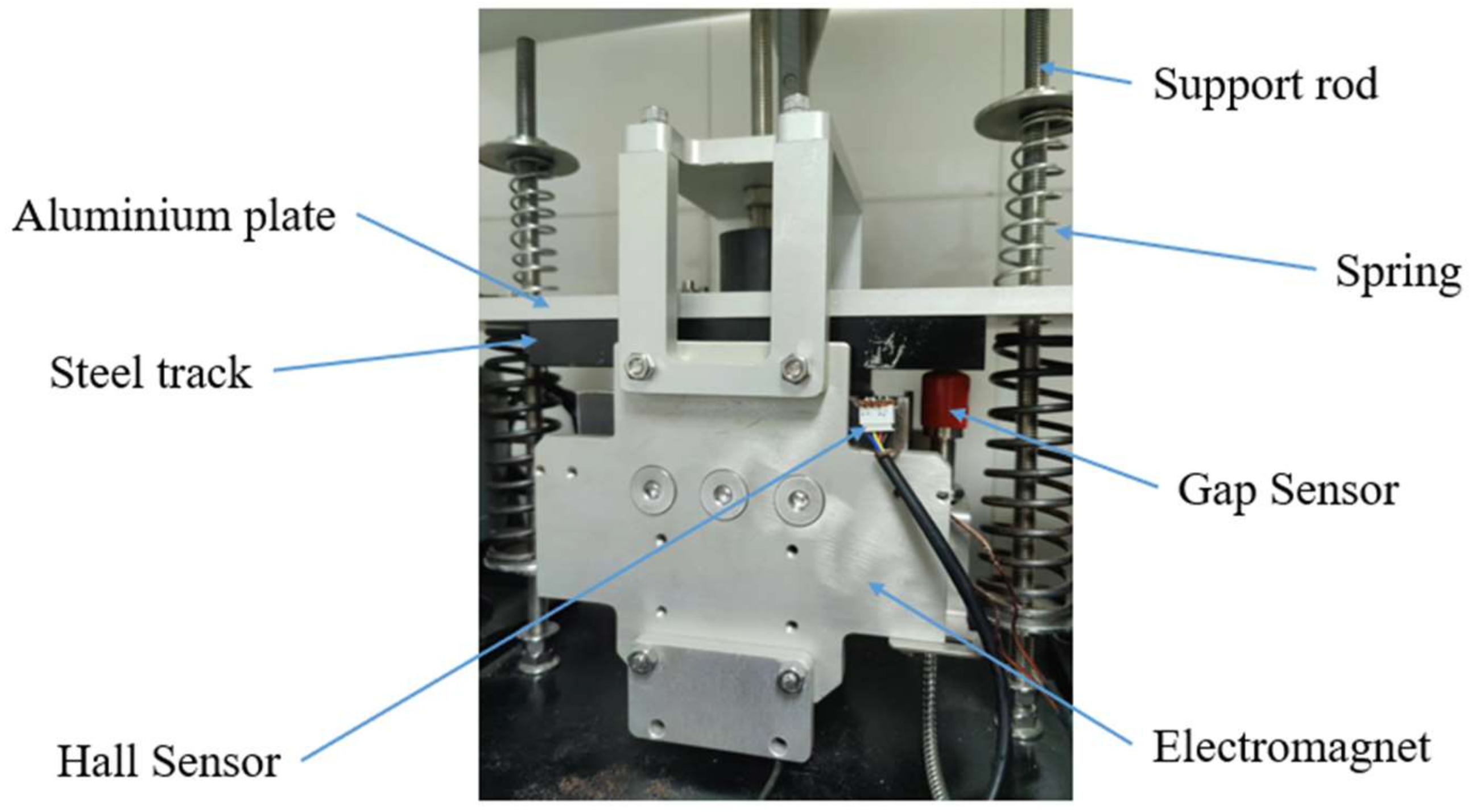
The track of the experimental platform was supported by low-stiffness springs on both sides, and the stiffness of the guideway was much greater than of the springs. Therefore, the deformation of the track was completely generated by the springs, whose stiffness was very low compared with a real maglev guideway. Therefore, this platform was ideal for studying vehicle–guideway coupled vibration problems. A picture of the magnetic suspension experimental platform is shown in
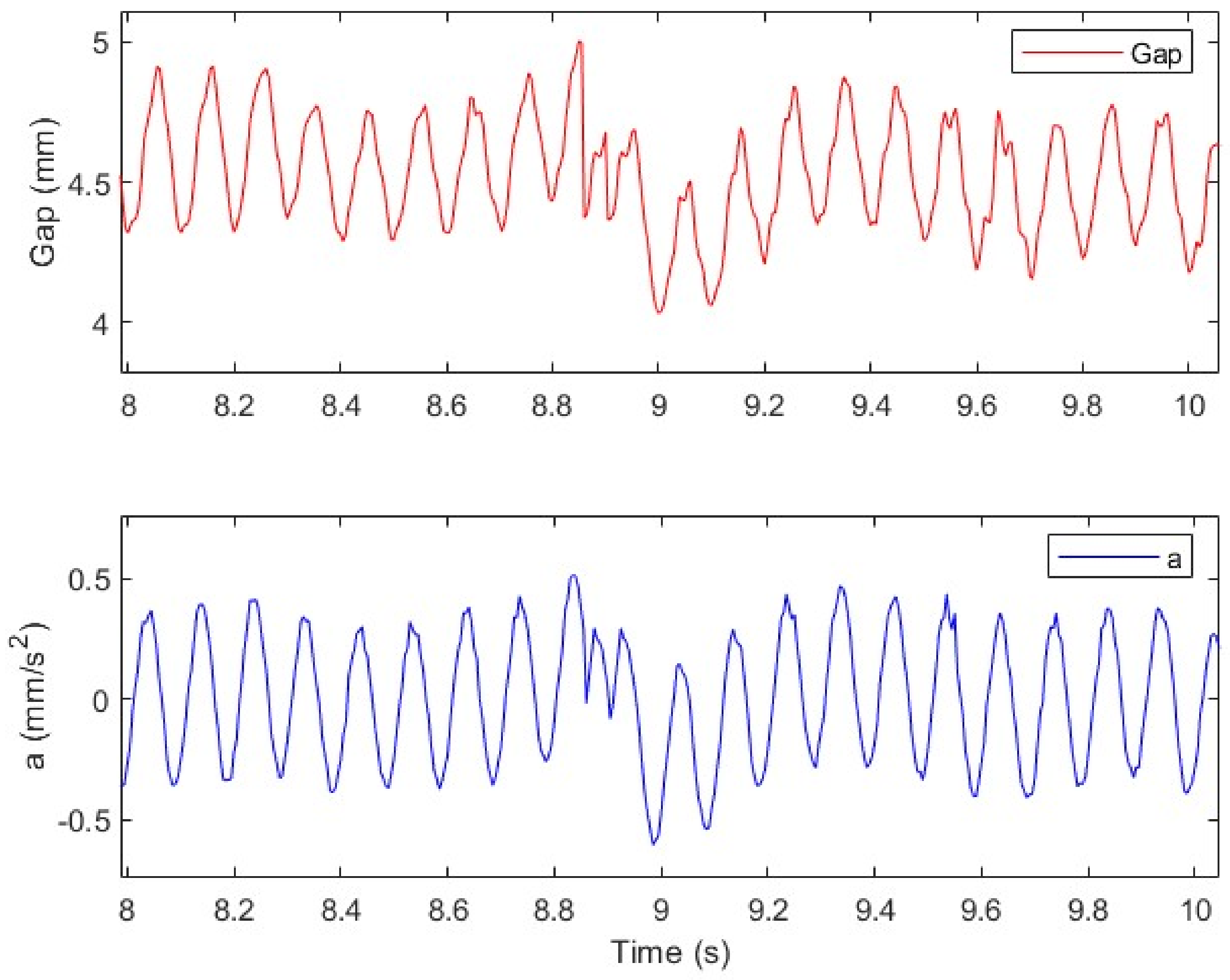
Figure 12. When the control method failed to suppress system vibration, the track was prone to self-excited vibration. A typical example is given in
Figure 13, where the gap and the acceleration of the track are plotted, respectively.
The track was first fixed with rigid constraints to test whether the control algorithm could achieve suspension on a rigid track. The control parameters were:
,
,
, and
, which satisfied the requirements of Equation (45). The poles of the system were
,
,
, and
.
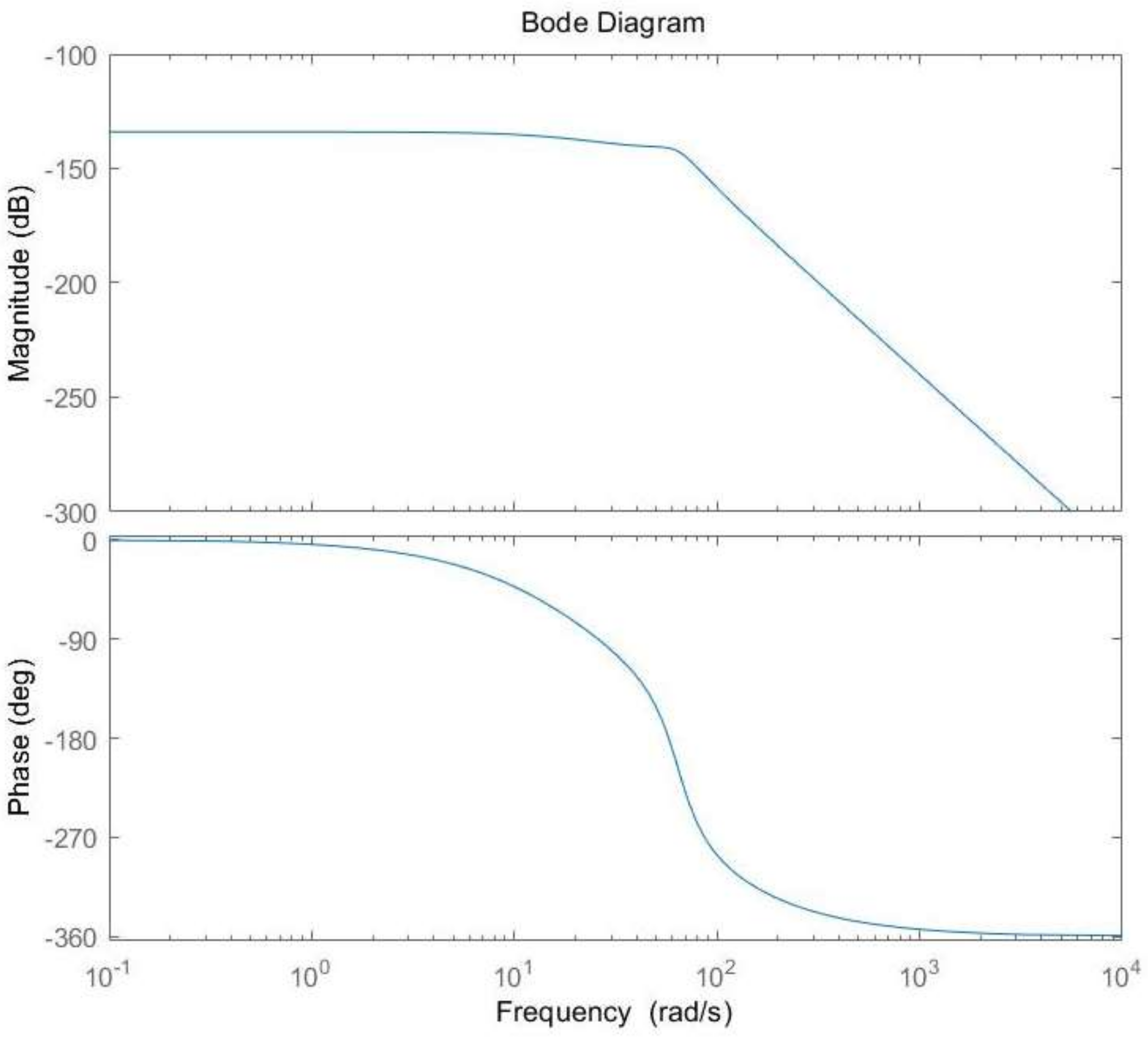
Figure 14 shows the Bode diagram of the system. As expected, the gain of the system in the low frequency band was about −134 dB, which satisfied the requirement of low gain. The phase shift of the system in the low frequency band was very small, which further proved the good stability of the system.
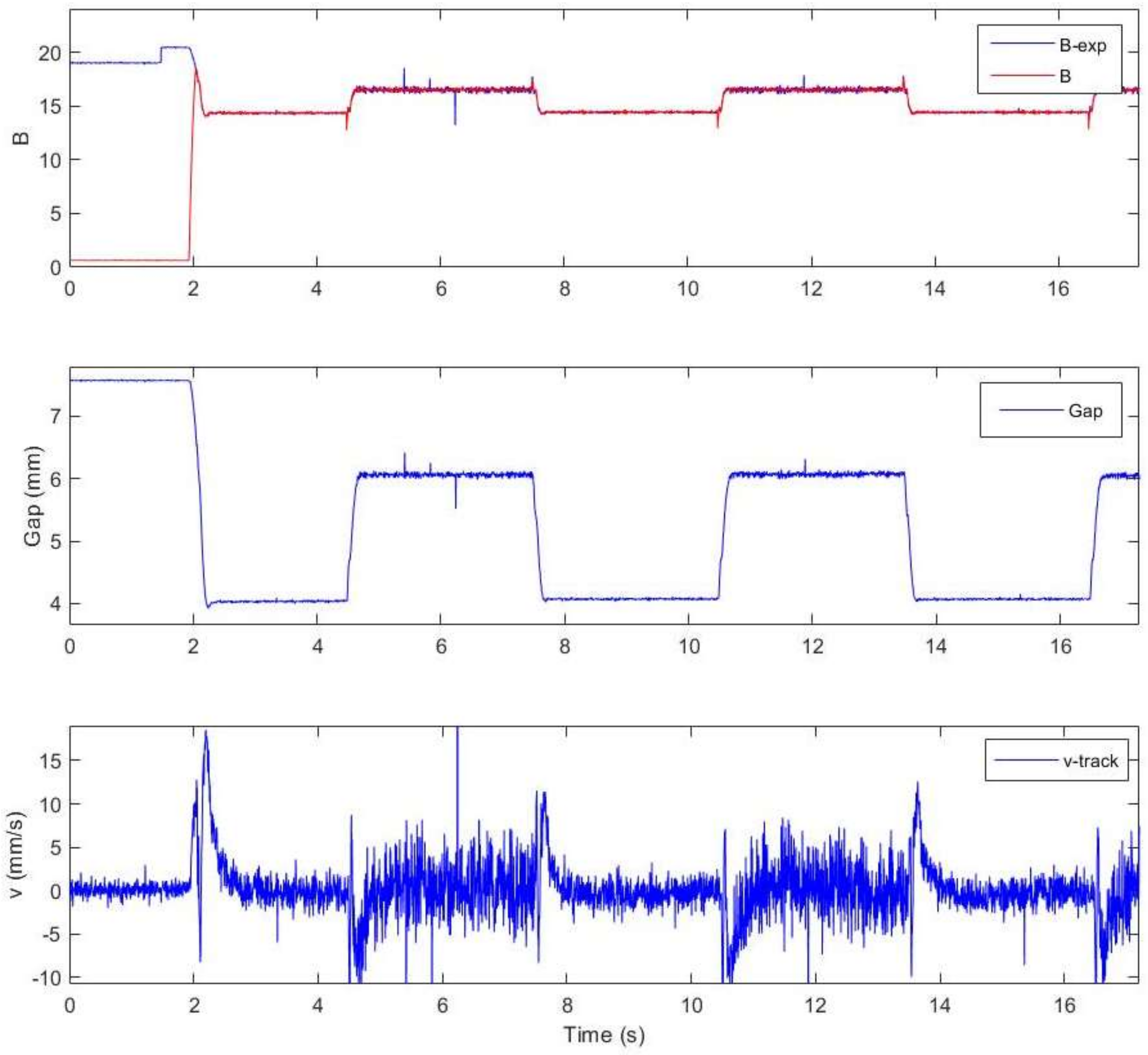
Figure 15 shows the effect of the control scheme proposed in this paper. The actual and expected magnetic flux, the suspension gap, and the vertical track velocity are plotted, respectively.
Meanwhile, a square wave signal with an amplitude of ±1 mm and a period of 2 s was applied to the desired suspension gap (5 mm). It can be seen that the suspension gap tracked the square wave signal well, with fast tracking speed, no overshoot, and no steady-state error. Meanwhile the actual magnetic flux also quickly tracked the expected magnetic flux, which showed that the performance of the magnetic flux loop was also reliable. However, the performance of this algorithm cannot be guaranteed under the flexible track condition, which needs further tests.
For the experimental platform, the stiffness of the track without constraint completely depended on the stiffness of the springs, which were quite low compared with the weight of the suspension load. In this case, the system was prone to the problem of vehicle–guideway coupling vibration, so the stability of the control algorithm under low stiffness could be effectively verified.
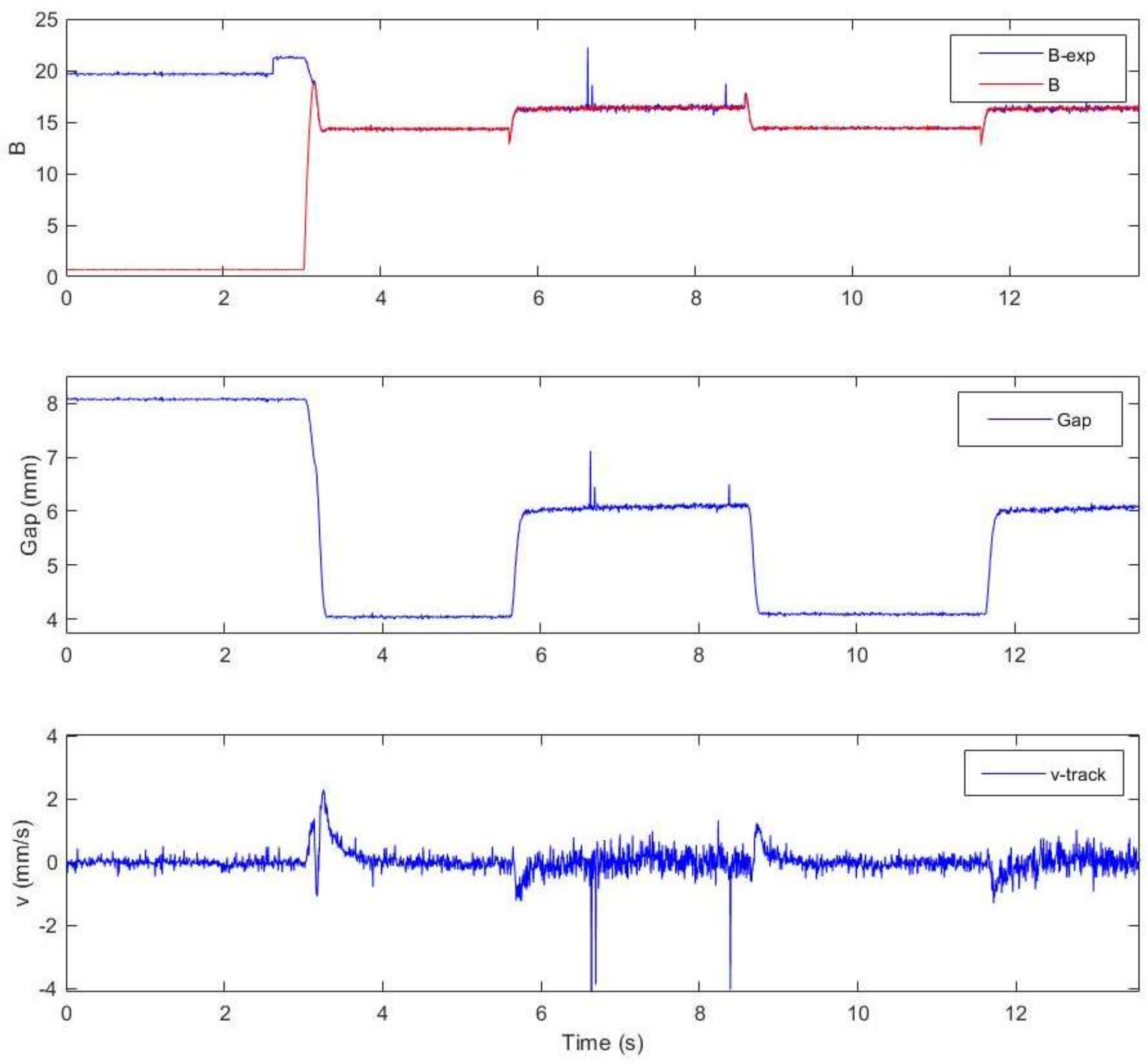
Figure 16 shows the actual magnetic flux, the expected magnetic flux, the suspension gap, and the vertical track velocity in the process of suspension. It can be seen that, although supported by low-stiffness springs, the suspension gap still quickly followed the desired gap with no overshoot and no steady-state error. Affected by disturbance of the electromagnetic force, the track suffered a downward speed and then quickly decelerated to zero, which showed that the coupling vibration never occurred. The experimental results proved that the algorithm had excellent control performance.
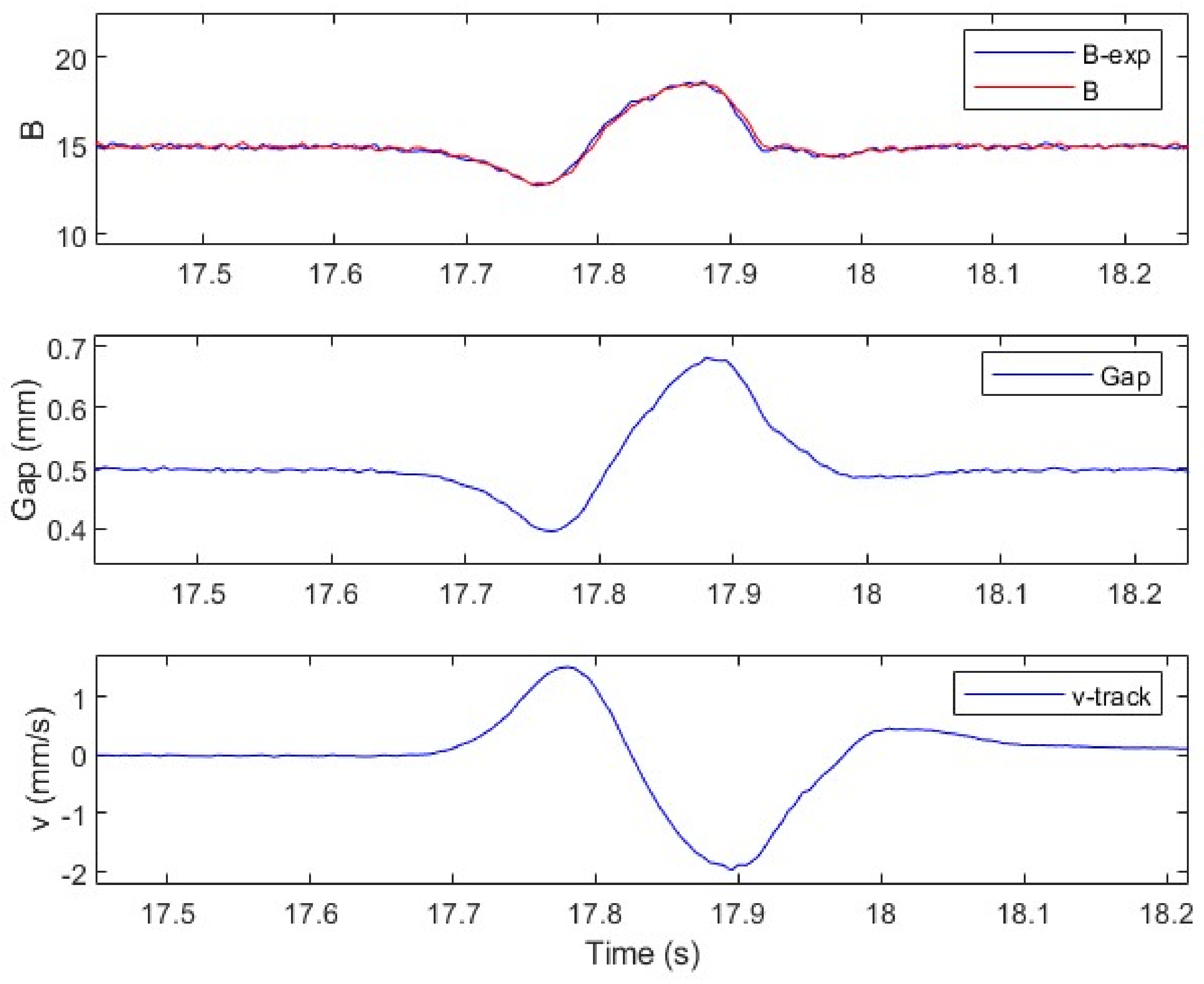
To further verify the anti-interference ability of the algorithm, a shock experiment was designed. A weight (about 0.6 kg) was placed about 70 mm above the track, and then the weight was dropped to freely fall and hit the track. The stability of the system was observed and experimental data recorded.
Figure 17 shows the suspension gap, the vertical track displacement, and the vertical track velocity during the impact. It can clearly be seen that the track moved downward after being hit, causing a sudden decrease in the suspension gap; and then the track bounced upwards and quickly returned to rest while the suspension gap returned to 5 mm within 0.3 s. This test indicated that the control strategy proposed in this paper could effectively deal with external disturbances in the case of extremely low track stiffness, and had a good effect on suppressing the vehicle–guideway coupled vibration with strong anti-interference ability.


