Article

Mechanism Design and Performance Analysis of a Sitting/Lying Lower Limb Rehabilitation Robot

Faculty of Mechanical Engineering & Mechanics, Ningbo University, Ningbo 315211, China
*
Author to whom correspondence should be addressed.
Machines 2022, 10(8), 674; https://doi.org/10.3390/machines10080674
Submission received: 15 July 2022 / Revised: 5 August 2022 / Accepted: 9 August 2022 / Published: 10 August 2022
(This article belongs to the Special Issue State-of-the-Art in Service and Rehabilitation Machines)

Abstract

:
To meet the various need of stroke patients’ rehabilitation training and carry out complex task training in real scenes, the structure of a lower limb rehabilitation robot with movements in the sagittal plane and coronal plane is usually complicated. A new sitting/lying lower limb rehabilitation robot (LOBO) with a simple mechanism form is proposed, which is designed based on a 2-PRR parallel mechanism. First, the kinematics, singularity, and condition number of the 2-PRR parallel mechanism are analyzed, which provides the basis for mechanism parameter design. Then, through the proportional–derivative control principle, real-time tracking of LOBO’s designed trajectory is realized. Finally, the length parameters of volunteers’ lower limbs are collected, and experimental verification is conducted in LOBO’s passive training mode. The experimental results show the feasibility of LOBO’s movement in the human sagittal and coronal planes. LOBO will help human lower limbs realize the synchronous continuous rehabilitation training of hip, knee, and ankle joints spatially, which could drive the rehabilitation movement of patients’ lower limbs in the sagittal plane and coronal plane in future clinical research. LOBO can also be applied to muscle strength training for the elderly to combat the effects of aging.

1. Introduction

Stroke is an illness that has a high potential of causing disability in the elderly [1]. More than 80% of stroke patients experience motor dysfunction due to decreased muscle strength [2], most commonly in the lower limbs [3]. Some studies have shown that the lower limb function and quality of life of stroke patients have been significantly improved after rehabilitation treatment [4]. Traditional rehabilitation training requires therapists to guide patients through rehabilitation in one-on-one sessions, which is inefficient and costly [5]. The contradiction between the large number of patients with limb dysfunction and the shortage of rehabilitation professionals in China needs to be solved urgently [6]. The lower limb rehabilitation robot, which can effectively improve the motor function of patients, has gradually become an important tool for the treatment of patients with lower limb dysfunction [7,8].
Fisiotek, developed as a single degree of freedom lower limb rehabilitation robot, is mainly driven by a simple DC motor to realize the passive training of patients’ hip and knee joints [9]. Although similar single degree of freedom robots have only a single movement mode, offering limited rehabilitation effects [10], they are widely used by hospitals because of their low price. On the basis of a single degree of freedom robot, lower limb rehabilitation robots with more than one degree of freedom have been developed rapidly in the past few decades, including wearable exoskeleton robots [11] and suspended rehabilitation robots. For example, Rewalk [12,13], composed of a pair of hip motors, a pair of knee joint motors, and a backpack integrating the control system and rechargeable batteries, can imitate the normal gait of the human body based on the preset movement model with an appropriate speed. Other typical wearable exoskeleton robots include Indego [14], HAL [15], Exo-H2 [16], and ROBIN [17]. Lokomat, a suspended rehabilitation robot, is a robotic gait orthosis with a weight-reducing suspension system. Lokomat is used in combination with a treadmill, and it guides the movement of patients’ legs according to the preset gait movement pattern [18]. Gait Trainer [19], developed by Rehastim (Berlin, Germany), provides power through the combination of two pedals, two rockers, and two cranks based on a double-crank rocker system [20]. Since most of these robots are only suitable for patients who can stand up, there are still challenges surrounding the lower limb rehabilitation of bedridden patients in the early stage of stroke.
Studies have found that sitting/lying lower extremity training can effectively reduce the load brought by the human’s trunk to the lower extremity, improve the stability of patients’ rehabilitation training, and also increase the range of motion of lower extremity joints [21], which is suitable for stroke patients in the early bedridden stage. Many sitting/lying rehabilitation robots support the lower limbs to facilitate rehabilitation training in the sagittal plane. For example, a sitting/lying lower limb rehabilitation robot based on a linear motor can realize the rehabilitation training of patients’ lower limbs in the sagittal plane by guiding flexion and extension of the limbs [22]. In addition, Physiotherabot [23] can realize rehabilitation training in the sagittal plane and coronal plane through a motor drive with a serial mechanism.
Compared to the serial mechanism, the parallel mechanism has a superior load-to-mass ratio and kinematic accuracy, as well as better dynamic characteristics and a higher stiffness and bearing capacity [24]. In recent years, due to its excellent characteristics, the parallel mechanism has attracted the attention of researchers [25] and been applied in many fields [26]. The parallel rehabilitation robot can realize the spatial movement of patients’ lower limb joints. For example, when a 3-UPS parallel mechanism is installed on a person’s thigh, the person’s thigh and mechanism are connected as a whole part, which can be considered as a 3-UPS/S parallel mechanism. Based on the asymmetric fully constrained parallel mechanism 3-UPS/S design, it can be used for hip joint assistance and rehabilitation [27]. Rutgers is an ankle rehabilitation robot based on Stewart parallel structure [28], which assists the free movement of patients’ ankle joints through the cooperative control of its six linear motors. Its mechanism has many degrees of freedom, which increases the complexity and cost of the robot control system. Arbot, a parallel rehabilitation robot, is used to meet the needs of plantar flexion/back extension, abduction/adduction, and valgus/varus of the ankle joint. Parallel mechanism has the inherent property of a small workspace [29]. At present, most parallel rehabilitation robots have two or three degrees of freedom, and focus on a single joint rehabilitation, such as hip, knee, or ankle joint.
In this study, a new type of sitting/lying lower limb rehabilitation robot is proposed. It is designed based on the characteristics of the 2-PRR parallel mechanism. Compared with the above parallel rehabilitation robots and serial rehabilitation robots, the proposed LOBO could realize the synchronous continuous rehabilitation training of hip, knee, and ankle joints spatially. It has a simple structure, which will be easy to control in future research. It is intended to be used for the rehabilitation of stroke patients in the early bedridden stage.

2. Range of Motion Analysis of Lower Limbs in Humans’ Sitting/Lying Position

To ensure that the patient is not accidentally injured during the recovery process, the angle of each joint must be strictly limited to the maximum angle of that joint’s motion. Table 1 presents the maximum angles of joint motion. Each lower limb has three degrees of freedom in the sagittal plane, namely, the rotation of the hip joint, knee joint, and ankle joint. In this study, the ankle joint axis is selected as the theoretical end point of the lower extremity, and each lower limb of the human body is simplified into a two-link model, as shown in Figure 1.
Let the length of the thigh be l1 and the length of the calf be l2. The fixed coordinate system is denoted as o0-x0y0z0, the coordinate system of the hip joint is denoted as o1-x1y1z1, the coordinate system of the knee joint is denoted as o2-x2y2z2, and the coordinate system of the ankle joint is denoted as o3-x3y3z3. Additionally, θi (i = 0, 1, 2) is the rotation angle of each joint relative to axis xi (i = 0, 1, 2), and θ3 is the rotation angle of the lower limb about axis z0, where counterclockwise rotation is defined as the positive direction. According to Table 1, considering that the human body is in the sitting position, the actual flexion and extension angle θ0 of the hip joint will be limited. In this paper, 0 ≤ θ1 ≤ 45°, 0° ≤ θ2 ≤ 45°, and −150 ≤ θ3 ≤ 0° are selected. The D-H method is used to calculate the space coordinates of the end of the ankle joint (xc, yc, zc), which can be expressed as Equation (1).
x c = l 2 cos ( θ 1 + θ 3 ) + l 1 cos θ 1 cos θ 2 + x 0 y c = l 2 cos ( θ 1 + θ 3 ) + l 1 cos θ 1 sin θ 2 z c = l 2 sin ( θ 1 + θ 3 ) + l 1 sin θ 1
The joint angle formula can be expressed as Equation (2).
θ 1 = arcsin ( E ) α θ 2 = arctan y c x c x 0 θ 3 = arccos F θ 1 ,
where E = G 2 + z c 2 + l 1 2 l 2 2 2 l 1 G 2 + z c 2 , F = y c l 2 sin θ 2 l 1 cos θ 1 l 2 , G = x c x 0 cos θ 2 , and α = arcsin G G 2 + z c 2 .
To adapt to people of different heights, two sets of values, l1 = 550 mm, l2 = 430 mm and l1 = 402 mm, l2 = 313 mm, are selected for spatial motion analysis and a Monte Carlo method was used to draw the three-dimensional motion range of lower limbs in the sitting position. In Figure 2a, the yellow–green areas indicate the range of motion of l1 = 550 mm and l2 = 430 mm, and the blue areas indicate the range of motion of l1 = 402 mm and l2 = 313 mm. In this paper, the ankle joint is required to carry out plane rehabilitation exercise at z = 200 mm, and the range of motion bounded by z 200 mm is selected, as shown in Figure 2a, and the xy projection of this bounded range of motion is obtained, as shown in Figure 2b.
According to the analysis of Figure 2b, in the sitting position, the maximum straight-line distance of lower limbs in the x direction is about 800 mm and the maximum straight-line distance in the y direction is about 655 mm. The designed working range of LOBO should be within this range.

3. Mechanical Structure Design

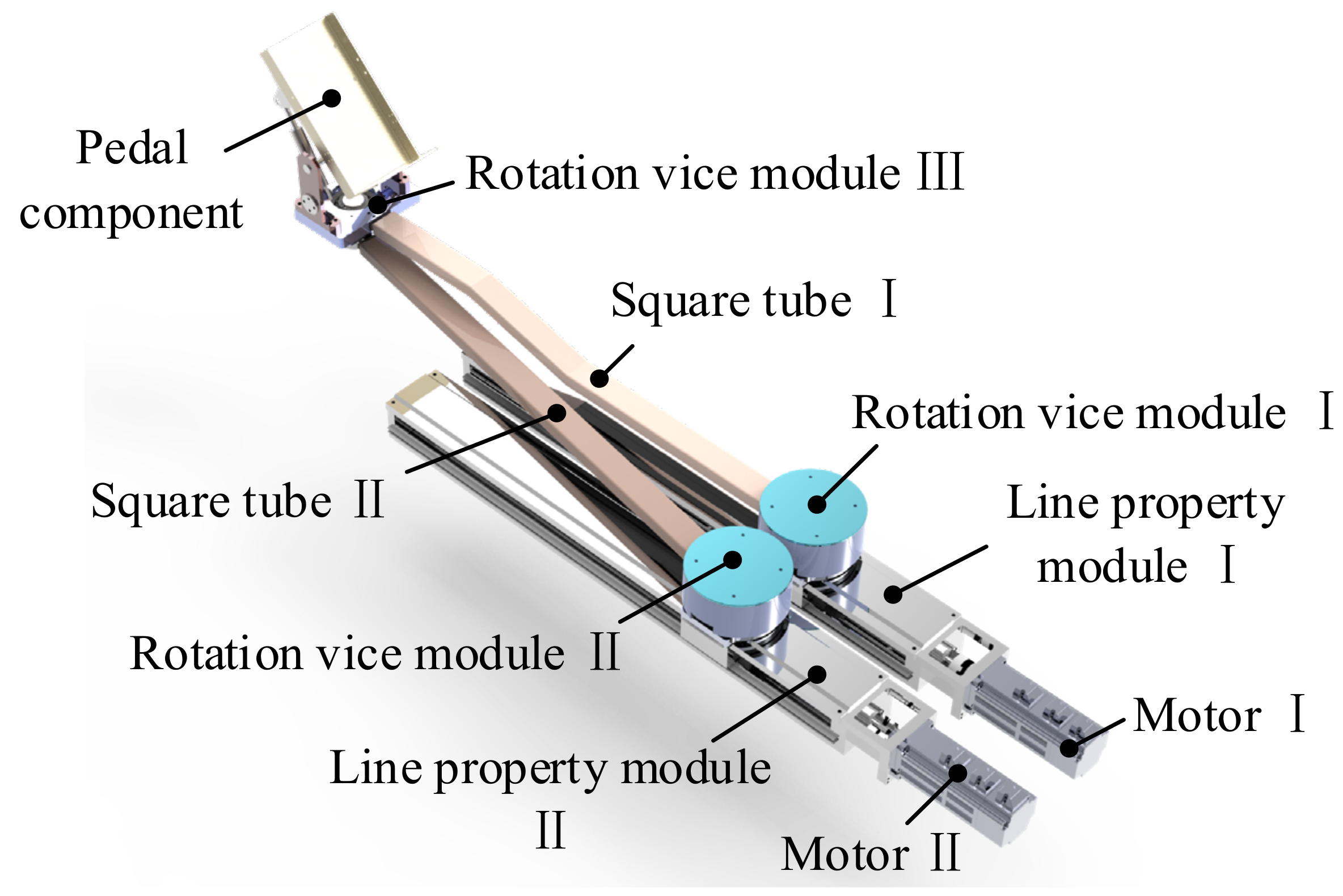
3.1. Mechanical Structure Description

As shown in Figure 3, LOBO’s overall structure is mainly composed of an underframe, lifting seat assembly, and lower limb rehabilitation training component. As shown in Figure 4, the lower limb rehabilitation training assembly includes motor I/II, linear stage I/II, rotation vice module I/II/III, square tube I/II, and pedal component. When the two motors operate at the same speed, the slider on the linear module drives the pedal rotation vice module I and the rotation vice module II forward/backward synchronously to achieve dorsiflexion/plantar flexion of the ankle and flexion/extension of the knee and hip joint in the sagittal plane. When there is a speed difference between the two motors, the pedal drives the patient to achieve abduction and adduction of the hip joint in the coronal plane.
The lifting seat assembly mainly includes a seat, electric push rod, and linear bearings. In the training process, the thighs, calves, and LOBO form a closed ring constraining A1A2A3A4, as shown in Figure 5. The patient can select the suitable closed ring by adjusting the seat height with different chain lengths A1A4.

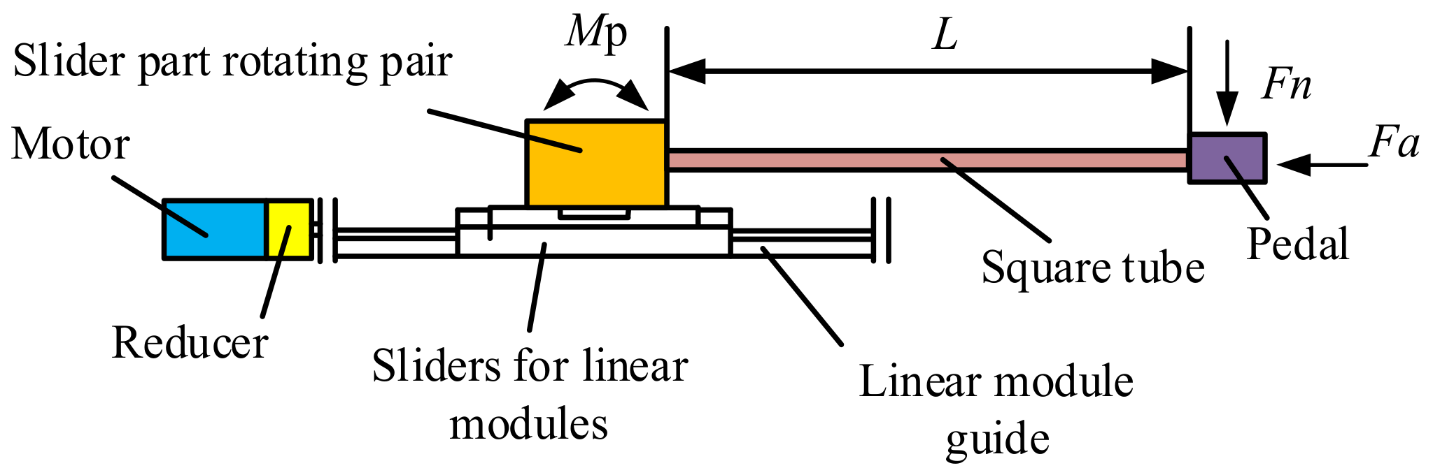
3.2. Selection of Motor Drive

3.2.1. Precision Linear Module Selection

As the lower limb rehabilitation training component adopts the 2-PRR parallel mechanism, the pedal for the patient’s foot will be suspended in the air. Meanwhile, considering the long length of the square tubes I/II used to connect the pedal component, the linear module is required to be able to withstand a large pitching moment. Assume that the length of the square tube on one side is 800 mm. The resultant force on the ends is Fn = 200 N. According to Figure 6, Mp represents the pitching moment, L represents the length of the square tube, and Fn represents the resultant force at the end. The pitching moment of the linear module is
M p = L × F n × K = 320   N m .
It is assumed that the straight-line working distance is S = 450 mm and the training time is t = 10 s. Then, the speed required by the pedal, v, can be determined by Equation (4), where K represents a safety factor; in this case, K = 2.
v = s t K = 45   mm / s
Based on the above information, the linear module model is selected as NDC86-1510-740-1-P-F0-S2 (3G Precise Machinery Co., Ltd., Tianjin, China). The rated pitching moment it can withstand is M p e = 622   N m   >   M p , and its effective linear displacement is Se = 610 mm > S.

3.2.2. Selection of Drive Motor and Reducer

The motor generates driving torque for the lower limb rehabilitation components. The rated driving torque will directly affect whether the whole mechanism can operate appropriately [30], according to Equation (5).
T = T 1 + T 2 + T 3 + T 4 ,
where T represents motor-generated driving torque; T1 represents torque generated by acceleration; T2 represents load torque (torque at constant speed); T3 represents preloading torque; T4 represents other torques.
Torque generated by acceleration, load torque, and preloading torque can be obtained through the formulas below:
T 1 = J L 2 π N 60 t T 2 = F a × I 2 π σ K T 3 = 0.05 ( tan β ) 0.5 F n × I 2 π * 10 3 ,
where N represents speed at the completion of motor acceleration, t represents accelerating period, JL represents the moment of inertia, F a represents the axial load, I represents the lead, σ represents the efficiency, F n represents the preload load, β represents the lead angle of the lead screw. It is assumed that F a = 500 N and σ = 80%.
Based on the above information, the selected motor model is SDGA-02C11AB (Tode Technologies Co., Ltd.,Changzhou, China), whose rated torque is 0.64 N∙m and rated speed is 3000 r/min. As the rated torque of the motor is too small, a reducer is selected—specifically, reducer model 60ZDF5-400T1 manufactured by Planetary Gearbox, which has a reduction ratio of 5:1. After the motor is equipped with the reducer, the actual torque of the output shaft is 3.2 N∙m and the actual speed is 100 mm/s.

4. Kinematics Analysis of Mechanism

4.1. Forward and Inverse Kinematics

The schematic diagram of the lower limb rehabilitation training component is shown in Figure 7, where AP and BP represent square tubes I/II, C1 and C2 represent sliders, and P represents the end point. When the two sliders move in a straight line on the guide rails, the end point P realizes two degree of freedom movement.
A new coordinate system is set up. It is denoted as O-XY, and its coordinate origin O represents the starting end of the guide rail of the linear module I. The distance between two parallel guides is a, and the lengths of the square tubes are, respectively, L1 and L2.
In the coordinate system O-XY, the coordinates of point P are (x, y), the coordinates of point C1 are (x1, 0), and the coordinates of point C2 are (x2, 0). It is easy to obtain the inverse solutions for x1 and x2 according to the geometric relationship:
x 1 = x L 1 2 y 2 x 2 = x L 2 2 ( y a ) 2 .
The coordinates of point P are obtained:
x = x 1 + L 1 cos α 1 = x 2 + L 2 cos α 2   y = L 1 sin α 1 = a + L 2 sin α 2 ,
where α1 is the included angle between AP and the x direction, and α2 is the included angle between BP and the x direction. The forward kinematics solution can be obtained as follows:
x = x 2 + L 2 M N + a D M 2 + a 2 y = a + L 2 a N M D M 2 + a 2 ,
where M = x 2 x 1 , N = L 1 2 M 2 a 2 L 2 2 2 L 2 , and D = a 2 + M 2 N 2 .

4.2. Jacobian Matrices and Singularity Analysis

4.2.1. Jacobian Matrix

A Jacobian matrix can not only directly express the mapping relationship between input parameters and output parameters, but the value of a Jacobian matrix is also an important index to determine the kinematic performance of the proposed mechanism. The Jacobian matrix is defined as the linear transformation of the operating speed of the mechanism and the joint speed, which can be regarded as the transmission ratio transmitted from each joint to the moving platform speed. In this paper, the Jacobian matrix is represented by J. When the joint velocity vector is known, the velocity vector of the operation space can be calculated according to the Jacobian matrix. When the velocity vector of the robot’s end-effector is given, the velocity of each joint can be calculated according to the inverse Jacobian matrix. The number of rows of the Jacobian matrix is equal to the dimension of robot motion in the operating space, and the number of columns is equal to the number of joints, so LOBO’s Jacobian matrix is a 2 × 2 square matrix. Taking the time derivative of Equation (7), we obtain:
( x x 1 ) x ˙ 1 = ( x x 1 ) x ˙ + y y ˙ ( x x 2 ) x ˙ 2 = ( x x 2 ) x ˙ + ( y a ) y ˙ .
Its matrix form is
x x 1 0 0 x x 2 x ˙ 1 x ˙ 2 = x x 1 y x x 2 y a x ˙ y ˙ .
Then, the following equation can be obtained:
x ˙ y ˙ = Q R x x 1 a ( x x 2 ) a x ˙ 1 x ˙ 2 ,
where Q = ( y a ) ( x x 1 ) ( y a ) ( x x 1 ) y ( x x 2 ) and R = y ( x x 2 ) ( y a ) ( x x 1 ) y ( x x 2 ) .
Finally, the Jacobian matrix of the 2-PRR parallel mechanism is obtained:
J = Q R x x 1 a ( x x 2 ) a .

4.2.2. Singularity Analysis

When the parallel mechanism is in the singularity position, the instantaneous degree of freedom of the LOBO’s mechanism will be uncertain, and the mechanism will lose its stability, transmission, and carrying capacity. Meanwhile, the driving force of the joint of the mechanism may tend to infinity, leading to the destruction of the mechanism. So, the singularity in the workspace should be avoided in the LOBO’s mechanism.
The singularity configuration of the parallel mechanism can be determined by the Jacobian matrices. When the Jacobian matrix det(J) = 0, there are three possible singularity situations: (1) AP is perpendicular to the X-axis, as shown in Figure 8a,e, (2) BP is perpendicular to the X-axis, as shown in Figure 8b,d, and (3) AP is collinear with BP, as shown in Figure 8c,f.
A limiting screw is added to the rotation of the first lower limb and the motion travel of the slider is restricted so as to avoid all three singularity configurations.

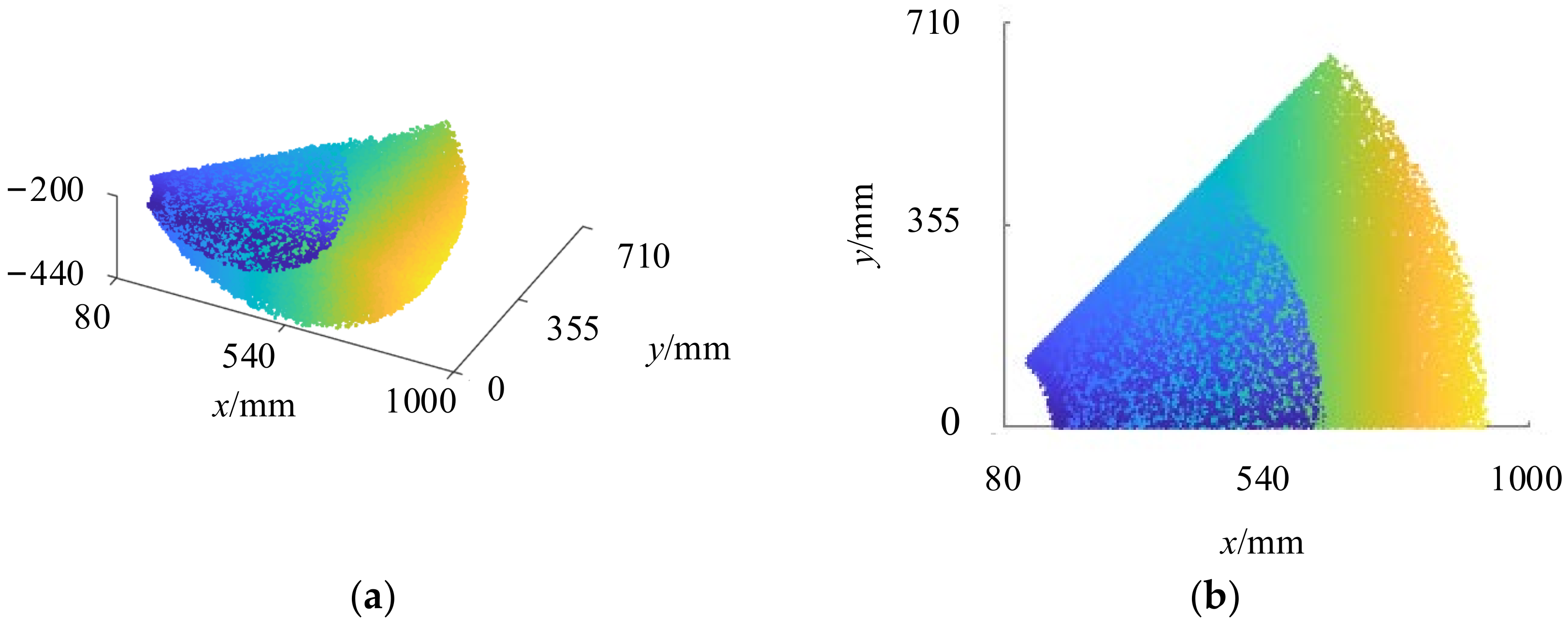
4.3. Condition Number

Judging whether the robot is in a singularity state by whether the determinant of the Jacobian matrix is equal to zero only qualitatively describes the robot’s kinematic performance; that is, it is either in a singularity or a non-singularity state. It cannot quantitatively evaluate how close the robot’s state is to the singularity state or the ability of the mechanism pose movement. The condition number of the Jacobian matrix, denoted by cond(J), is adopted as an index to measure the dexterity of the robot. When cond(J) = 1, the mechanism has the same kinematic ability in all directions, and it possesses the best flexibility. In this case, all singularity values of the Jacobian matrix are equal.
The condition number of the Jacobian matrix is expressed as
c o n d ( J ) = J J 1 ,
where J is the norm of the Jacobian matrix, and J 1 is the norm of the inverse of the Jacobian matrix.
When the value of the condition number of the velocity Jacobian matrix of the mechanism in its operating range is closer to one, the robot’s kinematic performance is better. Therefore, the actual size parameters of the prototype are substituted into the formula, and only the area of cond ( J )     30 is selected, as shown in Figure 9, whose coordinate system is the same as that of Figure 7. Figure 9a corresponds to the condition number when y > 0, and Figure 9b corresponds to the condition number when y < 0. It is found that the condition number increases non-linearly with the increase in y. Therefore, during trajectory planning, a large y value of the end-effector should be avoided.

5. Trajectory Planning

Trajectory planning refers to the design of the rehabilitation movement for rehabilitation training, which needs to be carried out in the workspace, namely the green area in Figure 10. After the completion of prototype development, the actual vertical distance between the hip joint and the ankle joint is measured to be about 250 mm. Therefore, the area z ≤ −250 mm is selected in Figure 2a. After coordinate transformation and translation, the blue–yellow area in Figure 10 is obtained through xy projection. By observing Figure 10, it can be seen that LOBO’s workspace contains most of the range of motion of patients’ lower limbs. Therefore, through reasonable trajectory design in the workspace, most of the training of patients’ joint angles can be satisfied, which proves that the parameter design of the lower limb rehabilitation robot is reasonable.
To realize a smooth motion trajectory, the displacement, velocity, and acceleration should also be designed to meet the requirements of smooth displacement and velocity and continuous acceleration. The experiments in this study take the left lower limb as the research object.
The specific parameters are as follows: the initial coordinates are (990 mm, 0 mm), the end coordinates are (1440 mm, 150 mm), β = arctan ( 150 0 1440 990 ) = 18.43 ° , the path length L is 474.34 mm, and the motion time t is 10 s. In the direction of the designed straight line, its displacement is defined as a 5th degree polynomial:
l ( t ) = a 0 + a 1 t + a 2 t 2 + a 3 t 3 + a 4 t 4 + a 5 t 5 ,
where ai (i = 0, 1, …, 5) represents the coefficients to be solved.
According to the known parameters, the displacement at the starting point is 0 mm, and the displacement at the ending point is 474.34 mm, satisfying the following constraints:
l 0 = 0 l 10 = 474.34 .
To meet the requirement of motion velocity continuity, that is, the velocity is zero at the starting point and the termination point, the constraint conditions are as follows:
l ˙ 0 = 0 l ˙ 10 = 0 .
To meet the continuous requirement of motion acceleration, that is, the acceleration is zero at the starting point and the termination point, the constraint conditions are as follows:
l ¨ 0 = 0 l ¨ 10 = 0 .
According to Equations (16)–(18), we can obtain:
l Ι = l ( t ) = 4.743 t 3 0.712 t 4 + 0.028 t 5 .
Displacements in the x and y directions are expressed as follows:
x ( t ) = l ( t ) cos ( β ) + 990 y ( t ) = l ( t ) sin ( β ) .
Similarly, to adapt to people with different heights, lII offers a shorter path than lI, and lIII offers an even shorter path:
l II = 5 t 1 3 0.75 t 4 + 0.03 t 5 l III = 3.59 t 3 0.539 t 4 + 0.02 t 5 .

6. Experiment and Evaluation

6.1. Experimental Setup

The LOBO used in the experiment to evaluate our pattern generation method consists of a relay board and four TSDA-C11A actuators and is coded using QT 5.9.7 based on the host computer (HP 15-bc011TX), other detailed parameters are shown in Table 2. The robot uses a proportional–differential (PD) control trajectory tracking method to implement the simulated rehabilitation movement. The experiment was conducted with the participation of 3 healthy volunteers. Table 2 contains the specific information of the volunteers. The process of volunteer I is shown in Figure 11. In each experiment, the training track of volunteer Ⅰ was l1, the training track of volunteer Ⅱ was l2, and the training track of volunteer Ⅲ was l3.
The specific principle is as follows: when the proposed program runs, the upper computer (HP 15-bc011TX) is used to read the real-time return value of the motor drive and process it to obtain the real-time position information xa(t) of the slider. Then, with the position information xd(t) of the next discrete point expected in the TXT document, the position deviation e(t) is obtained by using Equation (22). According to the position deviation e(t), the instantaneous velocity v(t) is calculated and sent to the motor through the serial port to realize real-time tracking.
v t = K p e t + K d d e ( t ) d t e t = x d t x a t ,
where Kp and Kd represent the proportional regulation coefficient and differential regulation coefficient, respectively.
To further verify the feasibility of the proposed mechanism, experiments are conducted with three volunteers. The process of volunteer I is shown in Figure 12. Table 3 contains the specific information of the volunteers.

6.2. Experimental Result and Evaluation

After the experiments, the collected actual slider position data of the three volunteers are imported into Excel for data processing, the plot function of MATLAB is used for plotting, and the comparison graph of the actual curve of the x value of the slider coordinate is obtained, as shown in Figure 13. Then, using the forward kinematics solution formula and the real-time position information of slider C1 and slider C2, the x value and y value of the end-effector are obtained, as shown in Figure 14.
To observe subtle differences, the curves in Figure 14a are differentiated along the x and y directions, and real-time deviations at each instant are plotted to obtain Figure 15. In Figure 15, the deviations in the x and y directions tend to increase with time at first and then decrease. Through the analysis, presumably because the time interval between consecutive speed instructions sent by the driver to the motor is short, when the required speed is high, the acceleration of the motor is insufficient to enable the motor to raise the speed to the required value in a short time, so the deviation is positively correlated with the speed.
Figure 16 shows the real-time tracking error of two sliders, that is, the difference between the actual position information at the current moment and the theoretical position information at the next moment. The velocity of the planned trajectory increases gradually and then decreases gradually, and the time interval between two consecutive discrete points is the same after the trajectory is discretized. Therefore, the greater the velocity, the greater the distance between the two discrete points. As a result, the real-time tracking error value in Figure 16 also increases at first, and then decreases.
Figure 17 shows the changes of the three angles over time. It can be seen that the curves are generally smooth and stay within the range of safe angles.
To sum up, the deviations in the x and y directions are strictly controlled within 10%, thus further verifying the feasibility of the mechanism.

7. Conclusions

In this study, a new type of sitting/lying lower limb rehabilitation robot based on the 2-PRR parallel mechanism is proposed, and the kinematics model of the 2-PRR parallel mechanism is analyzed. In order to make the working space of the machine adapt to people of different heights as much as possible, this paper adopts two groups of data of large and lower limbs, respectively, and draws the three-dimensional motion range of lower limbs under the sitting state of the human body with a Monte Carlo method. Then, the structure of the experimental prototype and the selection of related components are designed. According to the final actual size parameters, the condition number of the mechanism is analyzed. It is found that the condition number increases with the increase in y. Under the condition that the number of conditions approaches one, the workspace of the machine is selected, and a straight-line trajectory is planned, which can realize lower limb movement in the sagittal plane and coronal plane at the same time. Finally, based on PD real-time tracking control, experiments on the planned trajectories are conducted with three volunteers. By analyzing the experimental data returned by the drivers, the feasibility of both the PD real-time control and the mechanism is verified.

Author Contributions

Conceptualization, Y.F. and F.D.; methodology, F.D.; software, H.L.; validation, Y.F., F.D. and H.L.; formal analysis, H.L.; investigation, F.D.; writing—original draft preparation, Y.F.; writing—review and editing, F.D.; visualization, H.L.; supervision, F.D.; project administration, F.D.; funding acquisition, F.D. All authors have read and agreed to the published version of the manuscript.

Funding

This research was funded by the Natural Science Foundation of Zhejiang Province, grant number LQ21E050008; Educational Commission of Zhejiang Province, grant number Y201941335; Science and Technique Plans of Ningbo City, grant number 202002N3133; The Major Scientific and Technological Projects in Ningbo City, grant number 2020Z082; Research Fund Project of Ningbo University, grant number XYL19029; and the K. C. Wong Magna Fund of Ningbo University.

Institutional Review Board Statement

The study was conducted according to the guidelines of the Declaration of Helsinki, and approved by the Ethics Committee of Faculty of Mechanical Engineering & Mechanics, Ningbo University (protocol code [2022]LLSP(0310) and 2022.03.10).

Informed Consent Statement

Informed consent was obtained from all subjects involved in the study.

Data Availability Statement

Not applicable.

Conflicts of Interest

The authors declare no conflict of interest.

References

  1. Wu, J.P.; Gao, J.W.; Song, R.; Li, R.H.; Li, Y.N.; Jiang, L.L. The design and control of a 3DOF lower limb rehabilitation robot. Mechatronics 2016, 33, 13–22. [Google Scholar] [CrossRef]
  2. De Rooij, I.J.; Van De Port, I.G.; Meijer, J.G. Effect of virtual reality training on balance and gait ability in patients with stroke: Systematic review and metaanalysis. Phys. Ther. 2016, 96, 1905–1918. [Google Scholar] [CrossRef] [PubMed]
  3. Dharma, K.K.; Damhudi, D.; Yardes, N.; Haeriyanto, S. Increase in the functional capacity and quality of life among stroke patients by family care-giver empowerment program based on adaptation model. Int. J. Nurs. Sci. 2018, 5, 357–364. [Google Scholar]
  4. Almaghout, K.; Tarvirdizadeh, B.; Alipour, K.; Hadi, A. Design and control of a lower limb rehabilitation robot considering undesirable torques of the patient’s limb. Proc. Inst. Mech. Eng. Part H: J. Eng. Med. 2020, 234, 1457–1471. [Google Scholar] [CrossRef]
  5. Miao, M.D.; Gao, X.S.; Zhu, W. A construction method of lower limb rehabilitation robot with remote control system. Appl. Sci. 2021, 11, 867. [Google Scholar] [CrossRef]
  6. Wu, S.M.; Wu, B.; Liu, M.; Chen, Z.M.; Wang, W.Z.; Anderson, C.S.; Sandercock, P.; Wang, Y.J.; Huang, Y.N.; Cui, L.Y.; et al. Stroke in China: Advances and challenges in epidemiology, prevention, and management. Lancet Neurol. 2019, 18, 394–405. [Google Scholar] [CrossRef]
  7. Costandi, M. Rehabilitation: Machine recovery. Nature 2014, 510, S8–S9. [Google Scholar] [CrossRef]
  8. Wang, F.; Qian, Z.Q.; Lin, Y.Z.; Zhang, W.J. Design and rapid construction of a cost-effective virtual haptic device. IEEE/ASME Trans. Mechatron. 2020, 26, 66–77. [Google Scholar] [CrossRef]
  9. Deaconescu, T.; Deaconescu, A. Pneumatic muscle actuated isokinetic equipment for the rehabilitation of patients with disabilities of the bearing joints. In Proceedings of the International Multi-Conference of Engineers and Computer Scientists, Hongkong, China, 18–20 March 2009; pp. 1823–1827. [Google Scholar]
  10. Feng, Y.F.; Wang, H.B.; Lu, T.T.; Vladareanuv, V.; Li, Q.; Zhao, C.S. Teaching training method of a lower limb rehabilitation robot. Int. J. Adv. Robot. Syst. 2016, 13, 57. [Google Scholar] [CrossRef] [Green Version]
  11. Chen, B.; Ma, H.; Qin, L.Y.; Gao, F.; Chan, K.M.; Law, S.W.; Qin, L.; Liao, W.H. Recent developments and challenges of lower extremity exoskeletons. J. Orthop. Transl. 2016, 5, 26–37. [Google Scholar] [CrossRef] [Green Version]
  12. Hwang, S.H.; Sun, D.I.; Han, J.; Kim, W.S. Gait pattern generation algorithm for lower-extremity rehabilitation–exoskeleton robot considering wearer’s condition. Intell. Serv. Robot. 2021, 14, 345–355. [Google Scholar] [CrossRef]
  13. Long, Y.; Du, Z.J.; Wang, W.D.; Dong, W. Human motion intent learning based motion assistance control for a wearable exoskeleton. Robot. Comput.–Integr. Manuf. 2018, 49, 317–327. [Google Scholar] [CrossRef]
  14. Rodríguez-Fernández, A.; Lobo-Prat, J.; Font-Llagunes, J.M. Systematic review on wearable lower-limb exoskeletons for gait training in neuromuscular impairments. J. Neuroeng. Rehabil. 2021, 18, 1–21. [Google Scholar] [CrossRef]
  15. Chen, B.; Zhong, C.H.; Zhao, X.; Ma, H.; Guan, X. A wearable exoskeleton suit for motion assistance to paralysed patients. J. Orthop. Transl. 2017, 11, 7–18. [Google Scholar] [CrossRef]
  16. Vaughan-Graham, J.; Brooks, D.; Rose, L.; Nejat, G.; Pons, J.; Patterson, K. Exoskeleton use in post-stroke gait rehabilitation: A qualitative study of the perspectives of persons post-stroke and physiotherapists. J. Neuroeng. Rehabil. 2020, 17, 1–15. [Google Scholar] [CrossRef]
  17. Esquenazi, A.; Talaty, M.; Jayaraman, A. Powered exoskeletons for walking assistance in persons with central nervous system injuries: A narrative review. PMR 2017, 9, 46–62. [Google Scholar] [CrossRef]
  18. Yang, X.; She, H.T.; Lu, H.J.; Fukuda, T.; Shen, Y.J. State of the Art: Bipedal Robots for Lower Limb Rehabilitation. Appl. Sci. 2017, 7, 1182. [Google Scholar] [CrossRef] [Green Version]
  19. Morone, G.; Paolucci, S.; Cherubini, A.; De Angelis, D.; Venturiero, V.; Coiro, P.; Iosa, M. Robot-assisted gait training for stroke patients: Current state of the art and perspectives of robotics. Neuropsychiatr. Dis. Treat. 2017, 13, 1303–1311. [Google Scholar] [CrossRef] [Green Version]
  20. Calabrò, R.S.; Cacciola, A.; Bertè, F.; Manuli, A.; Leo, A. Robotic gait rehabilitation and substitution devices in neurological disorders: Where are we now? Neurol. Sci. 2016, 37, 503–514. [Google Scholar] [CrossRef]
  21. Chen, J.; Huang, Y.P.; Guo, X.B.; Zhou, S.T.; Jia, L.F. Parameter identification and adaptive compliant control of rehabilitation exoskeleton based on multiple sensors. Measurement 2020, 159, 107765. [Google Scholar] [CrossRef]
  22. Chrif, F.; Nef, T.; Lungarella, M.; Dravid, R.; Hunt, K.J. Control design for a lower-limb paediatric therapy device using linear motor technology. Biomed. Signal Processing Control 2017, 38, 119–127. [Google Scholar] [CrossRef]
  23. Eiammanussakul, T.; Sangveraphunsiri, V. A lower limb rehabilitation robot in sitting position with a review of training activities. J. Healthc. Eng. 2018, 2018, 1–18. [Google Scholar] [CrossRef] [PubMed] [Green Version]
  24. Mohanta, J.K.; Mohan, S.; Deepasundar, P.; Kiruba-Shankar, R. Development and control of a new sitting-type lower limb rehabilitation robot. Comput. Electr. Eng. 2017, 67, 330–347. [Google Scholar] [CrossRef]
  25. Jiang, Y.; Li, T.M.; Wang, L.P.; Chen, F.F. Improving tracking accuracy of a novel 3-DOF redundant planar parallel kinematic machine. Mech. Mach. Theory 2018, 119, 198–218. [Google Scholar] [CrossRef]
  26. Yang, Y.; Tang, L.; Zheng, H.Y.; Zhou, Y.; Peng, Y.; Lyu, S.N. Kinematic stability of a 2-DOF deployable translational parallel manipulator. Mech. Mach. Theory 2021, 160, 104261. [Google Scholar] [CrossRef]
  27. Yu, Y.; Tao, H.B. A parallel mechanism and a control strategy based on interactive force using on hip joint power assist. Int. J. Mechatron. Autom. 2014, 4, 39–51. [Google Scholar] [CrossRef]
  28. Girone, M.; Burdea, G.; Bouzit, M.; Popescu, V.; Deutsch, J.E. A Stewart platform-based system for ankle telerehabilitation. Auton. Robot. 2001, 10, 203–212. [Google Scholar] [CrossRef]
  29. Erdogan, A.; Celebi, B.; Satici, A.C.; Patoglu, V. ASSIST ON-ANKLE: A reconfigurable ankle exoskeleton with series-elastic actuation. Auton. Robot. 2017, 41, 743–758. [Google Scholar] [CrossRef]
  30. Giberti, H.; Cinquemani, S.; Legnani, G. A practical approach to the selection of the motor-reducer unit in electric drive systems. Mech. Based Des. Struct. Mach. 2011, 39, 303–319. [Google Scholar] [CrossRef]
Figure 1. Lower limb analysis of a healthy adult.
Machines 10 00674 g001
Figure 2. Range of motion analysis of ankle joint axis. (a) Lower limb range of motion bounded by z ≤ −200 mm. (b) The x-y projection of the bounded range of motion in (a).
Machines 10 00674 g002
Figure 3. The overall structure of LOBO.
Machines 10 00674 g003
Figure 4. Lower limb rehabilitation training component.
Machines 10 00674 g004
Figure 5. Closed loop diagram.
Machines 10 00674 g005
Figure 6. Static analysis of linear module.
Machines 10 00674 g006
Figure 7. Structure diagram of lower limb rehabilitation training module.
Machines 10 00674 g007
Figure 8. Singularity configuration of parallel mechanism.
Machines 10 00674 g008
Figure 9. Jacobian condition number.
Machines 10 00674 g009
Figure 10. Working range comparison.
Machines 10 00674 g010
Figure 11. Control assembly. (a) Relay board. (b) TSDA-C11A actuators.
Machines 10 00674 g011
Figure 12. Experimental demonstration process.
Machines 10 00674 g012
Figure 13. The value of x1 and x2 over time. (a) The terminal x1 value varies with time. (b) The terminal x2 value varies with time.
Machines 10 00674 g013
Figure 14. Terminal trajectories and y-value variation with time. (a) The end of the track. (b) The terminal x value varies with time. (c) The terminal y value varies with time.
Machines 10 00674 g014
Figure 15. The deviation of x and y values over time. (a) The deviation of the terminal x value. (b) The deviation of the terminal y value.
Machines 10 00674 g015
Figure 16. Track tracking error of sliders. (a) Track tracking error of slider C1. (b) Track tracking error of slider C2.
Machines 10 00674 g016
Figure 17. The participants’ joint motion curves. (a) The terminal θ1 value varies with time. (b) The terminal θ2 value varies with time. (c) The terminal θ3 value varies with time.
Machines 10 00674 g017
Table 1. The range of motion of human lower limb’s joint.
JointDatum PlaneMovementAngle Range (°)
HipSagittal planeFlexion (lying pos.)0~125
Flexion (sitting pos.)0~45
Coronal planeAbduction (lying pos.)0~45
Adduction (sitting pos.)0~45
KneeSagittal planeFlexion−150~0
AnkleSagittal planeDorsiflexion0~20
Flexion0~45
Table 2. Main technical aspects of the LOBO.
Control
Component
ModelBasic ParametersNumber
Upper computerHP 15-bc011TXi5-6300HQ CPU @ 2.30 GHz1
MotorSDGA-02C12BD0.2 KW, 36 V, 0.64 N.m4
Linear moduleNDC86-1510-740-1-P-F0-S2610 mm4
Speed reducer60ZDF5-400T15:14
ActuatorsTSDA-C11ARS-2324
Relay boardWF-16i-16oRS-4851
Encoder/2500 p/r4
SoftwareQT 5.9.7/1
Table 3. The range of motion of three volunteers’ joints.
VolunteerGenderThigh LengthCalf Length
Male560 mm450 mm
Male500 mm435 mm
Male480 mm390 mm
Publisher’s Note: MDPI stays neutral with regard to jurisdictional claims in published maps and institutional affiliations.

