1. Introduction
To produce cadastral precision maps regardless of GPS support, this navigation algorithm incorporates the method of transferring topographic orientation on geo-reference polygonal [
1], extended to a temporary network of triangles at each vertex; controlled optoelectronic stations are placed by a minimum crew of three collaborative mobile robots that are linked to transfer the georeferenced using an optical target acquisition system composed of a laser distance meter, a photoresistor node, a radio frequency collimator and a self-leveling Stewart table. The coordinated master–slave navigation of the robot unit crew has two ranges managed respectively by a peripheral navigation system (PNS) and an extensive navigation system (ENS). The first is for rough approach to targets and for obstacle avoidance, by detecting borders with ultrasonic perception and odometry [
2]. The second rank applies to deep search route planning [
3]. The measurement of angles and distances is obtained by reiteration to meet the sigma II criterion [
4,
5].
1.1. Navigation and Operating System
The navigation system software is an application that runs on an operating system that works as a virtual machine created expressly for the hardware of the robot units, which is installed on a base operating system that can be a Linux distribution or IoT equivalent. The application manages eight hardware subsystems—according to the mapping algorithm that integrates the principles of Tarry, Pledge [
6], and topographic orientation transfer (TORT)—to transform the geometric parameters produced by the metrology system in Eulerian graphs, which are the basis for deep search with which extensive navigation must exhaust network prospecting. The OS kernel manages client commands through thread agents to interpret, validate, execute, and manage threads between functions. Through an Interpreter agent, it receives client requests, segments them, reviews their syntax, looks them up in the dictionary, reviews the types and ranges of parameters, packs them up, and delivers them as inputs for functions, according to the configuration of the defined task scripts by the kernel. They are then delivered to an executing agent, which in turn calls each function involved with its respective parameters. At the same time, the content of the reports of reception, beginning, end, and suspension of the execution of orders for both software and hardware are followed by a thread follower agent.
1.2. Underground Navigation and Cadastral Mapping
In project settings with low-scale economy for underground operations, the coverage of the GPS service is often lacking [
7]. Under such conditions, inertial positioning systems on mobile platforms with bearing traction [
8] are not adequate to link navigation to an absolute reference, as is required to produce topographic planimetry and altimetry suitable for project index. Mapping is a process of massive scale and standardized precision, the costs of which are considerably affected in inaccessible environments of underground infrastructure with conventional methods [
9,
10], so indirect methods are usually used to the detriment of precision. The adaptation of the topographic orientation transfer to the proposed extensive navigation allows direct methods to be applied that separate the uncertainty associated with inertial peripheral navigation from the metrology process for mapping.
1.3. Peripheral and Extensive Navigation
The reduction of displacement and effective maneuvering time of the robot units [
11] of this proposal is based on the independence of the metrology process and acquisition of topographic objectives, with the following four guidelines:
- (1)
The conceptualization of the infrastructure network as an Eulerian biograph.
- (2)
Tarry’s modified deep search.
- (3)
Modified Pledge radial referencing [
12].
- (4)
Transfer of Topographic Orientation (TORT).
Together, they allow defining the position of the topographic objectives by transferring them as nodes to the network map, assigning them coordinates by triangulation, and then interpreting the network as a graph. During prospecting, while the team of robot units looks for discontinuities in the borders of the pipelines as milestones for the analysis of nodes, the position of each robot unit can always be determined by triangulation. The milestones found by the SNP are reported to the SNE to be classified and identified, comparing them in the map database to eventually be incorporated with their associated pipelines. The characterization of the nodes is achieved by identifying with the metrology system the number and synchronous radial order of the edge connections (modified Pledge criterion), and by means of the TORT it is possible to determine by which of them the node is entered or exited, to record the traffic status of each edge (Tarry criterion), which is the basis of the SNE deep search method and the advance criterion. This process applied cyclically generates a circuit of nodes that, when exhausted, contains all the network nodes.
2. Materials and Methods
2.1. Prototypes of Robot Units
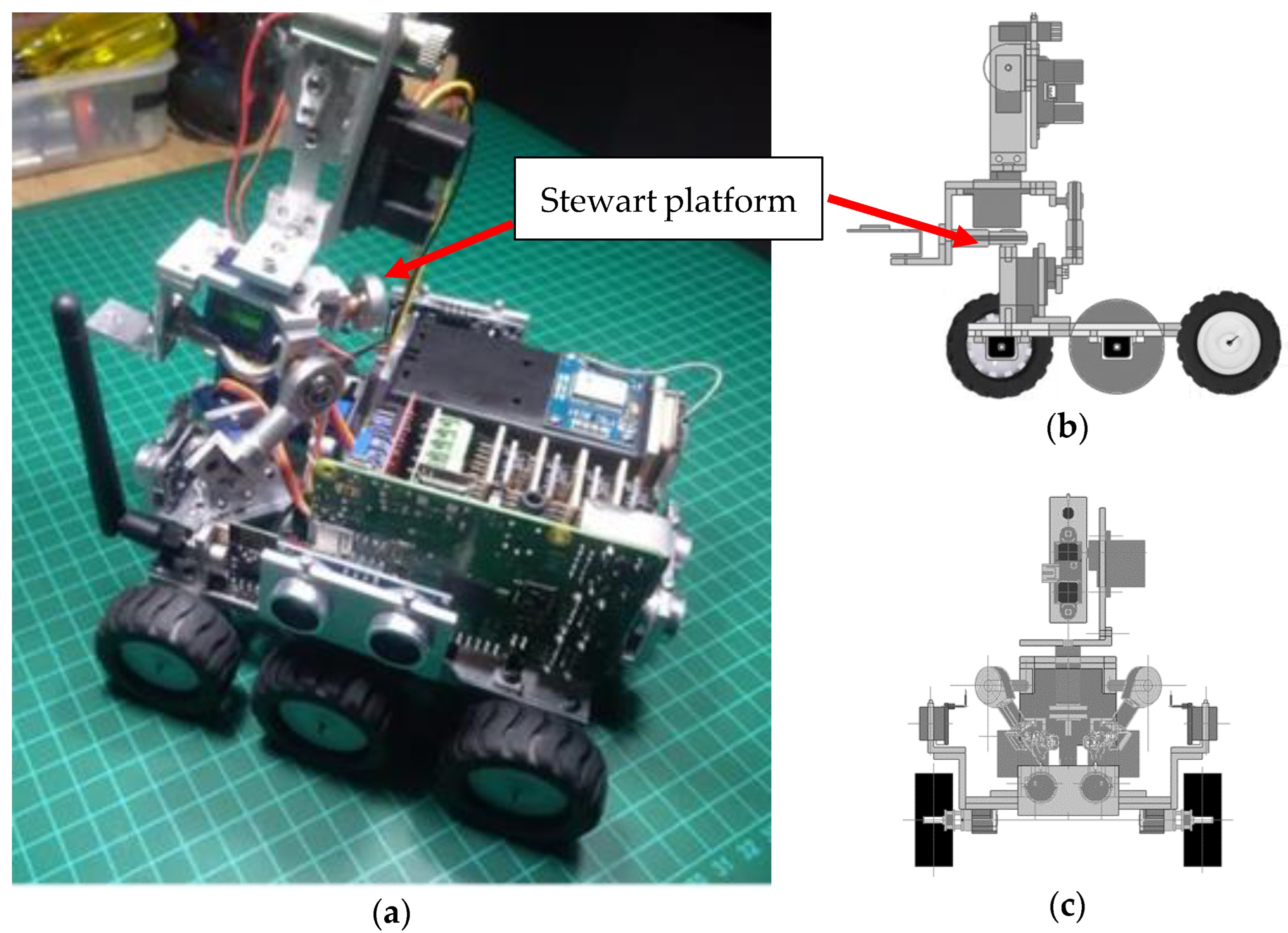
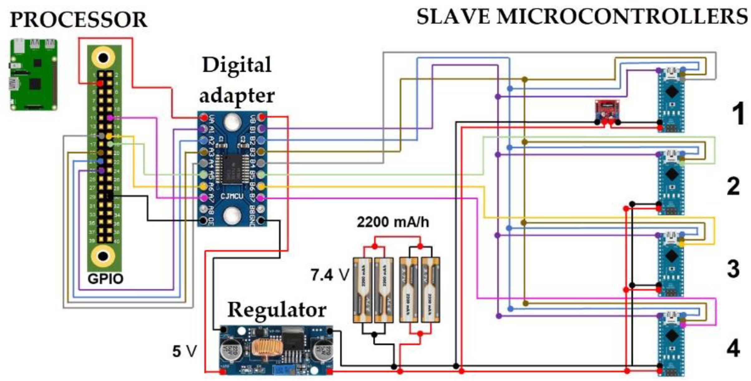
The prototype robots designed for the testing and validation of the navigation system use a Linux Raspbian distribution V3 processor and Microsoft Windows 10 IoT Core 17661 as the operating system, implemented as a virtual machine. The robotic operating system is also responsible for Navigation and Mapping. The hardware system consists of a Raspberry Pi 3 B+ motherboard, with a Broadcom BCM2837 1.2 GHz processor, and four Arduino Nano microcontrollers (ATmega 328P 16 GHz), which manage the sensors and actuators associated with each subsystem. The connection between the processor and the microcontrollers is a full duplex SPI (Serial Peripheric Interface) network, which allows the system to have a total of 7 sensors and 12 actuators, as shown in
Figure 1. The robot units can maneuver inside pipes of representative diameters of secondary networks adapted with a metrology system for topographic prospecting tasks. This is done according to the requirements of the lifting procedure based on polygonal circuits by triangulation, under the operation conditions of confinement in pipelines, including the programming of subsystems in slave controllers.
The systems integrated in each of the robot units include traction, peripheral perception, self-leveling (parallel architecture), metrology (and target acquisition) and radio frequency communication, and power management. Due to their close relationship, the ultrasonic traction and peripheral perception systems reside in the memory of a single microcontroller, while the remaining three systems reside separately, with each one in a microcontroller. Each of these microcontrollers is configured as a slave in a full duplex SPI network and contains a specialized task application with the ability to receive parameters and send results reports to the master unit.
2.2. Surveying Map and Metrology
The TORT is a conventional static reference method between points and axes based on laser and topographic triangulation; it does not require GPS support, and in short lengths, it does not need geodetic correction. In the field, this method can be carried out with mechanical–optical tools under static collimation conditions (visibility between the references) [
13,
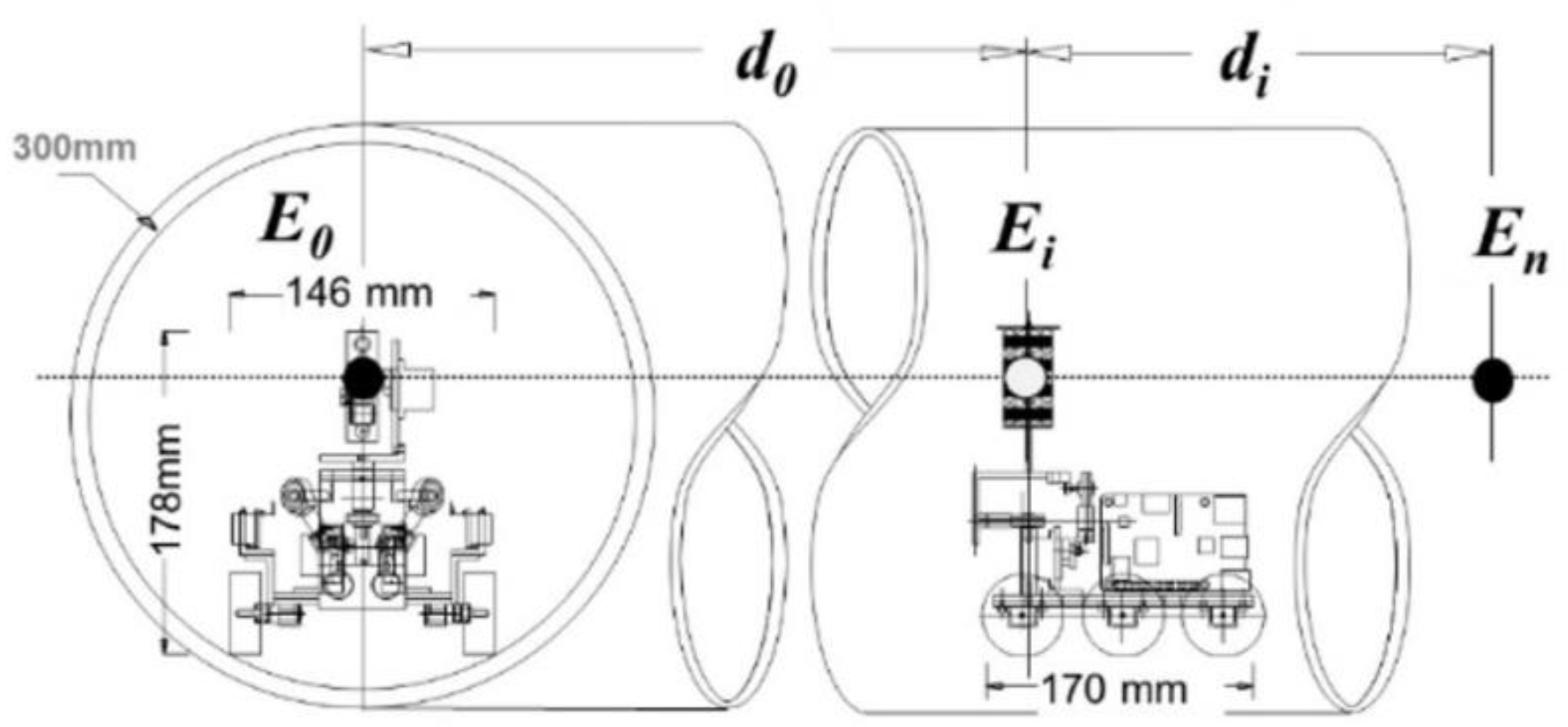
14]. The TORT procedure is slow compared to some lidar systems but achieves adjustable regulatory accuracy. The proposed incorporation of TORT in parallel to inertial navigation separates the uncertainty from the rough approach to the objectives, making the product independent of the metrology process. To start the TORT procedure, two validated georeferenced points are required as stations for the status of the slave units. The procedure consists of extending the reference network gradually by adding nodes by triangulation. During this operation, two of the three robot units must remain static on validated georeferenced points, while the third changes position to a surveying landmark. To triangulate, three parameters must be determined: (1) the azimuthal angle of the vectors formed between the two validated nodes and the target and their distances, and the (2) radial and (3) longitude measurements, both of which must be performed under an asymptotic condition with respect to the tangent plane in the points of reference (see
Figure 2 and
Figure 3). Once the angle and distances are known, the target coordinates can be calculated and processed in the map database. To guarantee the asymptotic reference of the topographic metrology system, a self-leveling Stewart platform is used that, by means of two independent orthogonal kinematic chains, regulates the inclination of the metrology platform, controlling a servomotor with the feedback of an accelerometer, as shown in
Figure 4.
2.3. Kinematics Model of Stewart Platform
Stewart’s platform is a parallel robot [
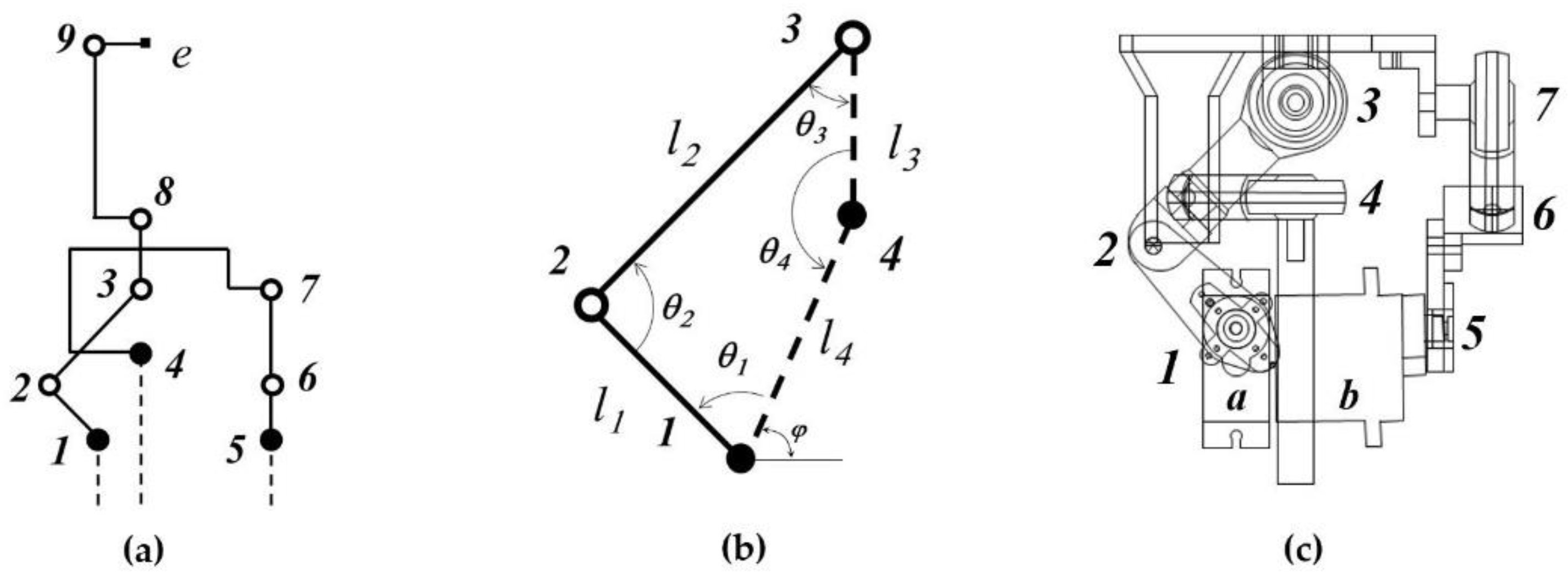
15]; the prototype is a tripod with two kinematics chains with four bars and four joints (see
Figure 4a,b): two fixed to the bench (1,4) and two mobile (2,3). Two are of spherical type (3,4), whilst the other two are cylindrical (1,2). The orthogonal arrangement of the chains and their two spherical joints minimize the magnitude of mutual affectation.
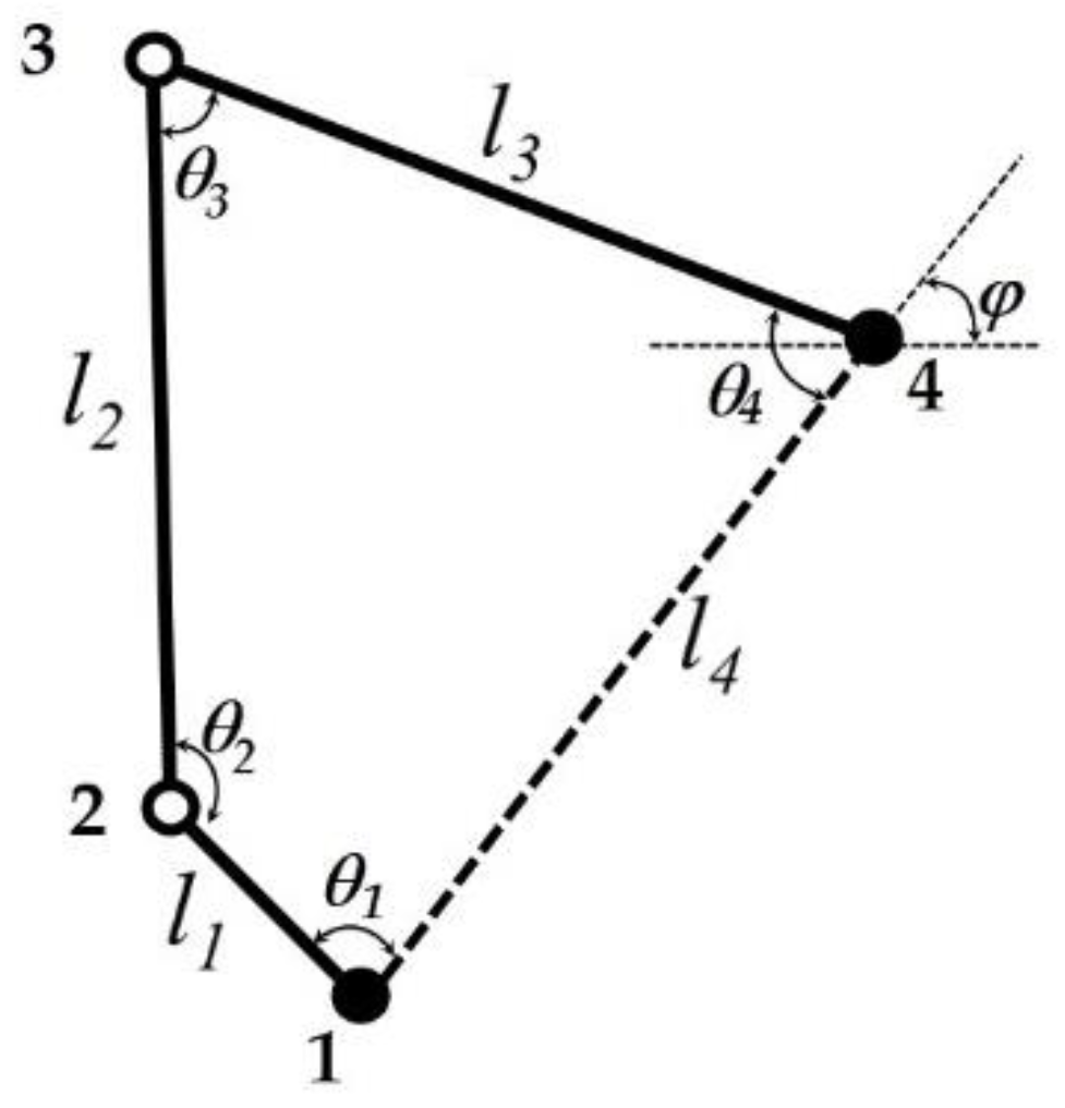
In the four-bar kinematic chains with two fixed joints, the positions of the mobile joints 2 and 3 of the angles between the links (
θ1, θ2, θ3, θ4; as shown in
Figure 4b) are defined by setting one of two parameters: (a) an angle between their links or (b) the position of one of the mobile joints. Given the restrictions of a closed chain, the first case follows direct kinematics, and the second case is the inverse. The control variable in the prototype is the angle
θ1, associated with joint 1, on whose axis of rotation the arrow of the actuator is installed [
16,
17,
18]. The dimensions for the links are
l1 = 0.0240 m,
l2 = 0.0785 m,
l3 = 0.0650 m, and
l4 = 0.079 m, with
φ = 55.3°
The output variable is the angle of inclination of the platform (
θ4); our analysis is focused on this variable and the position of the mobile joint 2, given by
For the distance between joints 2 and 4 (
), Equation (3) applies from known positions:
The angles
θ2 and
θ4 can be obtained as
Using
l2, l3, and segment
p2p4, the angular displacement for
θ3 can be obtained as
The position of the mobile joint 3 is
The other case of interest is when the angle inclination of the platform (
θ4) is known and
θ1 and the rest of angles and joints positions must be specially calculated, as shown in
Figure 5.
When angle
θ4 is defined, the rest of the angles (
θi) and the positions of the mobile joints 2 and 3 can be calculated as follows, in a process which is analogous to the above. The mobile position joint 3 is given by
The distance between joints 2 and 4 (
) can be obtained as
The angle
θ2 can be expressed by
Defined the position of the movable joint 3, and known the lengths of the links
l1, l2, l3, l4 and the positions of the fixed joints 1 and 4. To determine the angles
θ1, θ2, θ3, and
θ4, by means of the law of cosines, all interior angles of the triangles defined between the joints 1, 2, 3 and 1, 3, 4 are determined. From the sum of the partial attachment angles of
θ1 and
θ3, they will be defined:
where:
Using the triangle formed by elements the
l1,
l2 and segment
p1p3, the angular position for
θ2 can be expressed by:
With the Equations (1) to (16), the position for all links can be determined in different phases of an operative cycle.
2.4. Peripheral Navigation Mode
To control the direction and speed of advance during the prospecting, the PNS manages the microcontroller of the peripheral perception and traction system, which is associated with the six gear motors of the driving bearings and four ultrasonic distance sensors, placed cardinally in the chassis of the robot units. During the movement, the PNS oversees avoiding obstacles and detecting discontinuities in the border formed by the walls of the pipelines. Mapping accuracy is derived from collimation, distance, and angle instruments, as well as the number of independent, non-iterative operations required. The requirements for cadaster [
19], fulfilled under controlled conditions, can change when increasing the number of steps in an operation, which affects the systematic errors related to the segmentation of traverses to adjust the range of distance sensor range, angle encoder sensitivity, and coplanar auto-leveling [
20].
2.5. Graph-Based Map Production
The ENS formulates the map exploring the network, considering it as an imperfect labyrinth which as redundant paths (islands), creating an interpretable circuit as an Eulerian graph with a node for each bifurcation or directional change of its edges. By adding the direction of circulation to the edges, it becomes a directed graph, suitable for the deep search necessary to create the Tarry circuit with the nodes of the network. The double direction of circulation in the prospecting of the network pipelines guarantees the existence of an Eulerian circuit; however, additional procedures are required to discover that particular circuit, which is the objective of the ENS when guiding the prospecting by controlling the frequency and the direction of traffic.
2.6. Tarry-Pledge Algorithm
There are strategies that optimize various aspects of deep search; however, their application in this case is limited, because it cannot be assumed that enough characteristics of the network are initially known to be able to construct an adequate graph; however, the time and message complexity of Tarry’s algorithm is competitive. Its three rules are as follows: (1) When starting from a node, a step register will be made in the connection with the edge that will be traversed; (2) When arriving at a node, a passage record will be made in the connection with the edge that has been travelled; (3) In the selection of the edges to be covered, the unexplored edges will be advanced first, secondly through the one-way routes, and thirdly through the edge through which the node was reached. By adding the selection weight criterion according to the modified Pledge radial orientation to the algorithm, it is possible to differentiate the edges associated with a node, preparing them to be linked to the absolute reference using TORT. Choosing the radial sense of Pledge produces different partial circuits, but with equivalent end results.
2.7. Acquisition of Survey Objectives
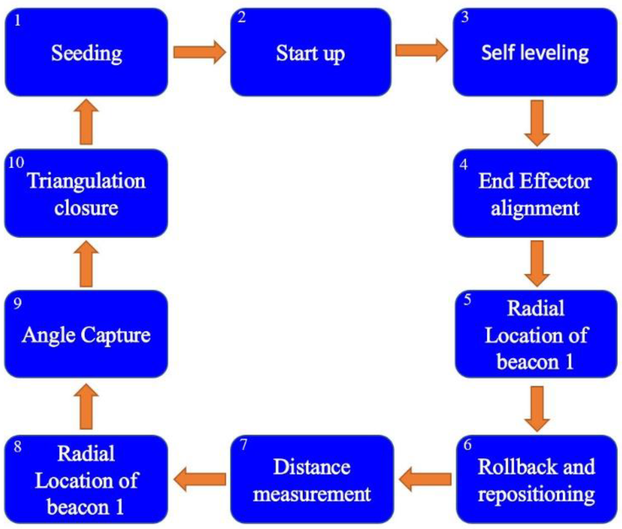
The SNE orders the acquisition of topographic objectives for the identification of the points where the collimation will focus during the measurement of distances and angles, which will define the nodes and edges. Meanwhile, the approach of the robot units to the targets is guided by the PNS. Considering a crew composed of a Master Robot Unit (MRU) and two Slave Robot Units (SRU1 and SRU2), the target acquisition cycle is described in
Figure 6.
The cycle starts with the seeding of robot units in the static starting position, with the Master Robot Unit (MRU) and the Slave Robot Unit 1 (SRU1) on the two validated reference link nodes, with the power supply active. Step 2 is starting up the basic sensor and actuator start-up test. Step 3 is self-levelling of platform of the slave beacon and the metrology module. Step 4 is the alignment of the final effector of the metrology arm perpendicular to the leveling platform; then, the radial location of beacon 1 is made via the MRU searching the SRU1 and 2 by means of a radial laser scan. The MRU activates the laser emitter and rotates the servomotor 1 of the metrology module, whose axis is perpendicular to the platform, which generates a rotation of the two links of the manipulator arm, normal to the platform, starting from the 0° position and ending at 180°, with the following parameters:
If, in this trajectory, the laser hits the opto-electrical sensors of the SRU1 beacon, the latter detects it and sends a “target” warning by radio frequency to the MRU, which stops the rotation of servomotor 1; the angle is recorded.
If, on the other hand, the total 180° scanning path of the laser ends without hitting a target with the opto-electric sensors of the SRU1 beacon, then the MRU changes the vertical orientation of the laser emitter, rotating the servomotor 2 (whose axis is parallel to the platform) one degree; the horizontal scanning cycle is then repeated.
This cycle is repeated until the target beacon is hit, or the servomotor 2 has rotated 120° (vertically).
If this happens, the search procedure is interrupted, and the MRU assumes that SRU1 is in a position out of range. Next, the MRU sends a backtracking and repositioning order to the SRU1, up to 10 times, trying to detect it again before aborting the operation. During the horizontal scanning procedure, when the opto-electrical sensors of the SRU1 beacon detect the ace of the MRU laser emitter, it sends a radio frequency “target” warning to the MRU, which stops the rotation of servomotor 1; the angle is recorded.
Step 6 is rollback and repositioning, wherein the SRUs change their position, approaching the MRU, to enter their range of measurement scope. The SNE indicates the direction of advance, and the PNS approaches the ERUs to the new point. Step 7 is distance measurement, which involves verifying the target on the SRU1 beacon and the MRU, and determining the clearing distance between the metrology platform and the beacon. Next, the IR laser sensor is activated, which is oriented parallel to the axis of the laser emitter, at a perpendicular distance of 22 mm, to measure this distance 10 consecutive times, in order to meet the sigma II criterion. The next parameter to determine is the angle formed by the three robot units, for which the auto-levelling command is executed again.
After the URM receives the confirmation notice from SRU2, it executes the search procedure via cylindrical scan of the beacon of SRU2 by the radial location of beacon 1 (step 8). When SRU2 is located, the MRU records the rotation angle of servomotor 1; now, the “target” is verified, which represents the angle formed by the three robot units with a vertex in the MRU (step 9), and given the triangulation closure with the current positions of servomotors 1 and 2, the MRU determines the distance to the beacon at SRU2. With the data of the distances MRU–SRU1 and MRU–SRU2 and the angle SRU–MRU–SRU2, the coordinates of the new nodes of the geo-reference network are calculated based on the law of cosines.
If the ultrasonic sensors encounter obstacles, the microcontroller application evaluates the change of direction option by searching synchronously for free peripheral areas. If no transit alternatives are detected, the URM returns with the crew to the previous node and re-evaluates the direction of advance. If the master unit cannot detect an advance route or cannot move, it proceeds to shut down the secondary systems of the entire crew except the communication one, and repeatedly sends a forced station report to the supervision unit and is put on hold for a new command.
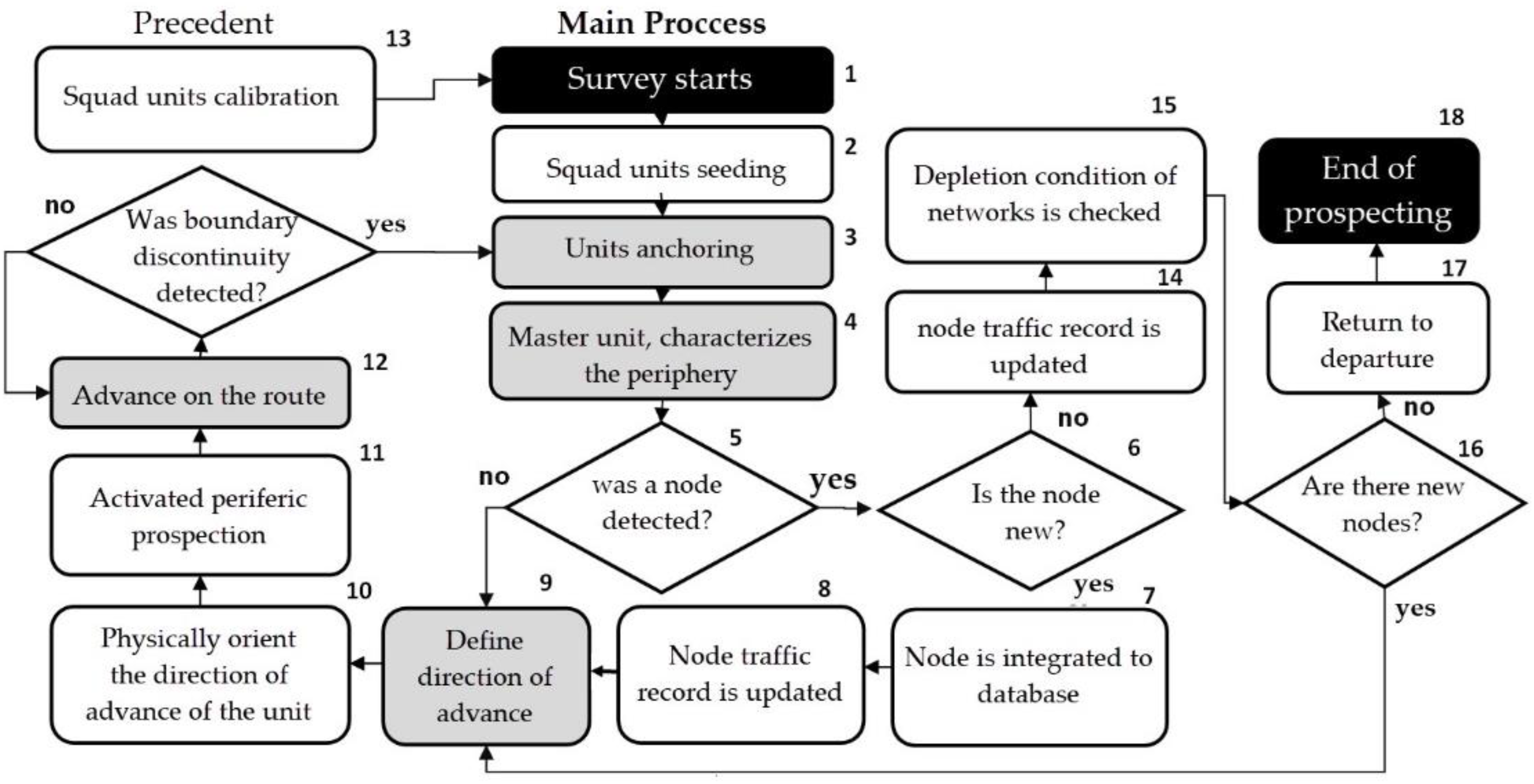
2.8. Navigation Algorithm
Alternating the functions of the ENS and the PNS, the navigation algorithm guides the progress of the units and processes the network graph, following the flow diagram in
Figure 7.
3. Numerical Experiment
Considering the fundamental aspects of the hypothesis, two experiments were carried out. The first had the objective of quantifying the quality of the data produced, comparing a physical control network of known dimensions and representative geometry against the data produced by the mapping system from the same network. Since this physical test is of limited extension with respect to the average infrastructure networks in the field (kilometer scale), a second stage of extensive-scale tests was executed with virtual replicas of real networks of known metropolitan areas, focusing on the performance of the algorithm logic when dealing with larger and complex databases.
For the physical validation test of the navigation system, a group of three prototypes of dedicated robot units was manufactured (two SRUs and one MRU), designed for the unavailability conditions of the GPS service (see
Figure 1) and the confinement in 12” diameters or larger representatives of municipal scale pipelines and typical auxiliary structures. The units were equipped with all the resources required by the navigation system to produce maps, without hermetic protection. Prototypes include a Broadcom 2.1 GHz 64-bit main processor with an SPI network for five 16 MHz 16-bit microcontrollers, managing eight connected sensor and actuator subsystems.
The virtual machine of the S.O. was installed on a Linux Raspbian 3.2 distro, 01-2020. The units have an approximate weight of 1.1 kg including batteries, and a total enclosure of 148 × 170 × 176 mm, as shown in
Figure 8.
The drive system direction of the units is sliding [
21], with six independently rotating, non-steerable bearings [
22]. The operation of the robot units is autonomous for up to 4 h, without requiring communication, control lines, or power supply.
Network for Validation by Physical Test
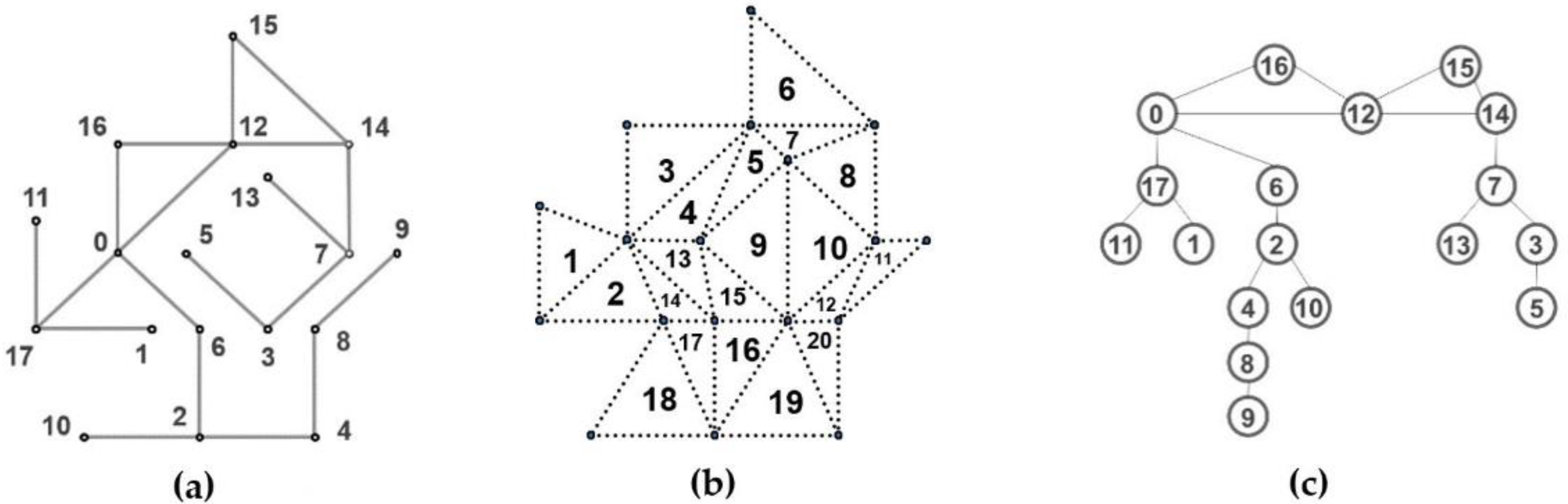
The mapping test network was built following the typical configuration of the geometry of secondary distribution hydraulic networks (open and closed mesh joints as shown in
Figure 9a). Topologically, it is composed of three trees and two cycles (
Figure 9c), with 18 nodes and 19 edges, all oriented in two directions. The diameter of its ducts is 12”, to facilitate manual access and seeding of the robot units. With 19.8 m of longitudinal development, it covers an area of 15 m
2. It was installed on a concrete surface with a uniform slope. The strength of the test network was traced by triangulation on a redundant control mesh with 20 triangles, as shown in
Figure 9b.
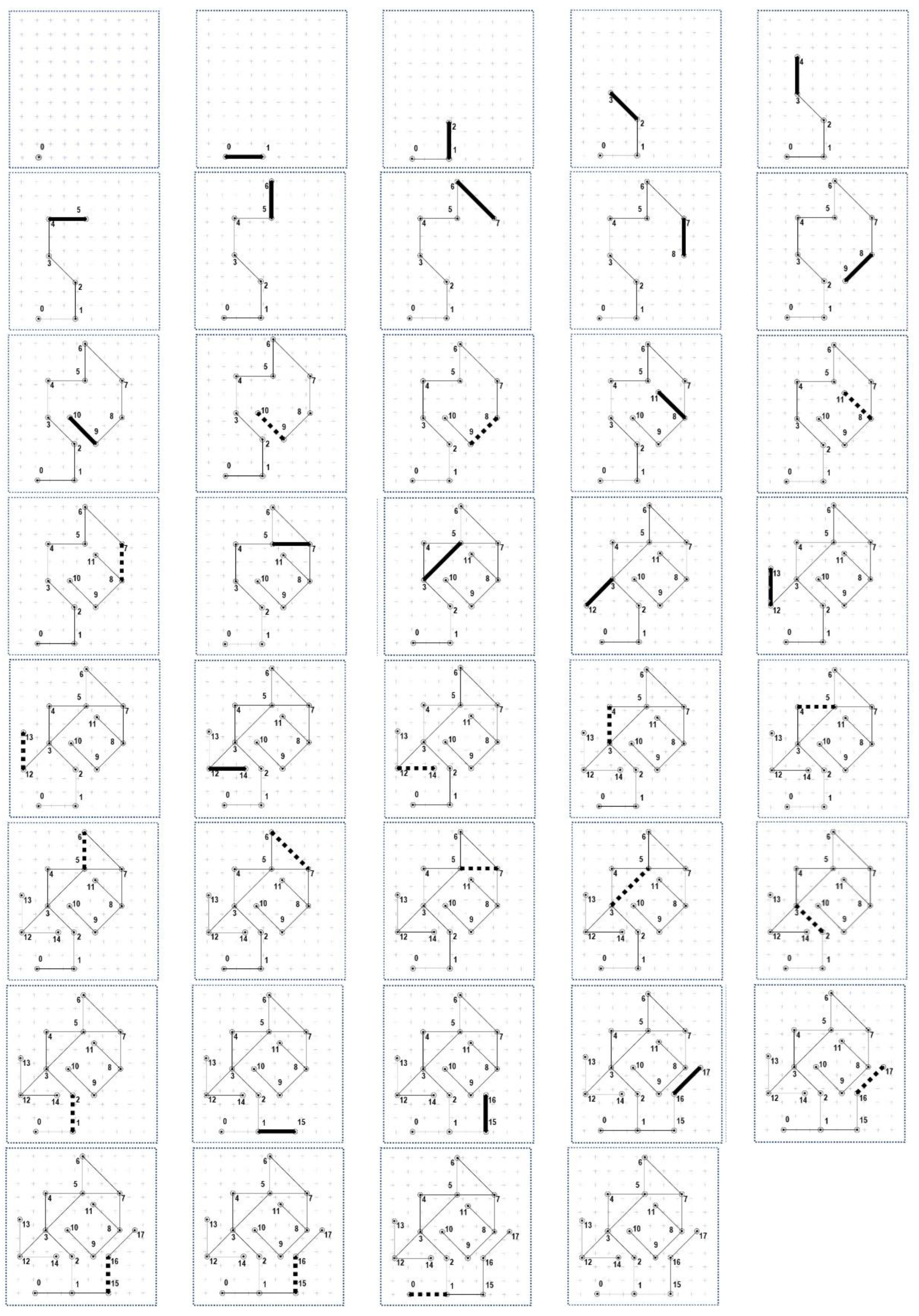
To generate the network R00, the infrared and ultrasonic sensors were calibrated in the three robot units and manually positioned in series on node 0 (see
Figure 9c), with a separation of 15 cm between them. Prospecting was carried out using the navigation algorithm from
Figure 7; the results are shown in
Figure 10, where the circuit contains return paths marked with dotted line edges.
Table 1 shows the total prospecting circuit vector (CPT) for the sequence node to node for the network R00, containing the 19 nodes of the network. The vector is formed by the visited nodes of 39 elements, which implies that 20 nodes were visited without acquisition of new data.
As an indicator of algorithm efficiency for a particular network R00, the Transit Index (IT) was defined as the quotient of the number of nodes in the CPT vector (NV) divided by the total number of nodes in the network (NR). The IT indicates how many times the total prospecting path is greater than the total length of the network. In the case of a network without leads, the IT would be equal to the unit. Specifically in the test network R00, the IT is 39/19 = 2.052; this implies that the network was traversed approximately twice to complete the survey, which coincides with the theorem of the Eulerian graphs. However, if the range of the distance sensor is less than the average edges, the number of operations increases multiplied by the number of robot units that execute the prospection, affecting the mismatch error of the nodes.
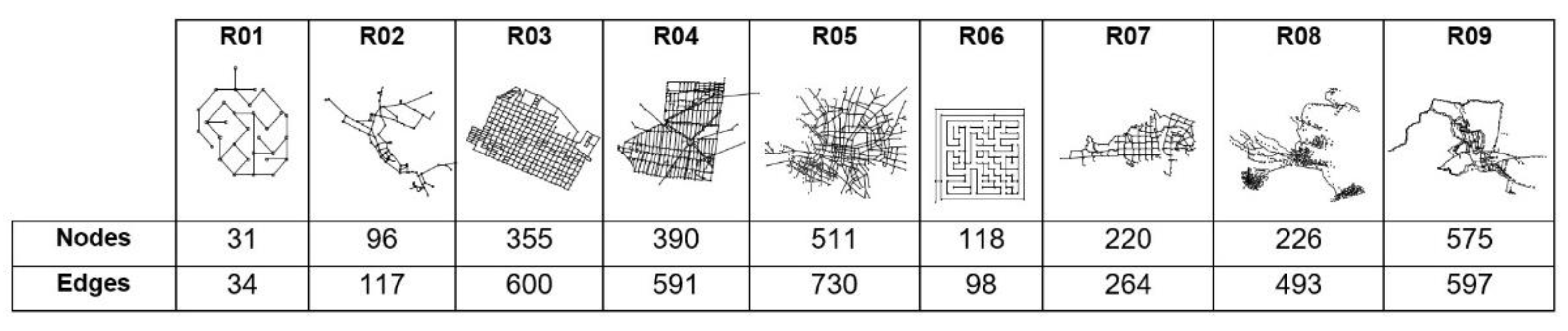
For the second stage of testing, nine network models were prepared, of different density and connectivity. These are shown in
Figure 11, together with the quantification of their modes and edges, with the largest being the R05 with 730 edges. Network R01 is an extension of the physical control network (R00), which maintains straight and 45° deflections to facilitate angle comparison. The R02, R08, and R09 networks represent rural areas, with the first being low-density and the other two being interconnections of several smaller systems. The R07 network is an interconnection of secondary networks in Quito, Ecuador. R06 is like a mini-mouse test maze. The remaining networks come from conurbation areas of Mexico: R05 is a secondary network in a north-eastern city, the R04 network is a high-density hydrometric control sector in a central city, and the R03 network corresponds to a high consumption sector in a northeastern city.
4. Results
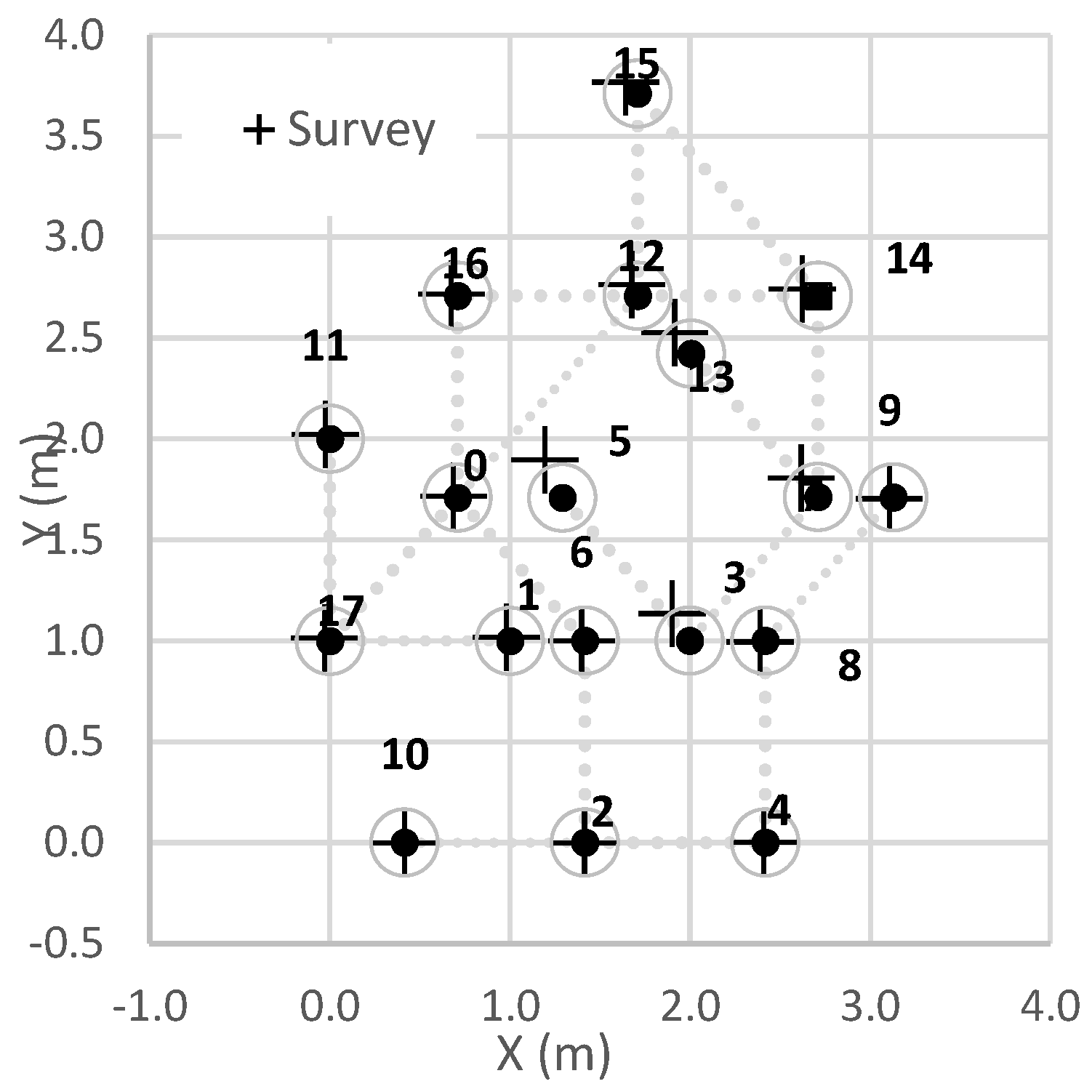
The first test allows evaluating the quality of the data produced by the mapping based on the offset error of its nodes, as shown in
Figure 12, where the coordinates of the nodes of the control mesh and those of the map have been superimposed.
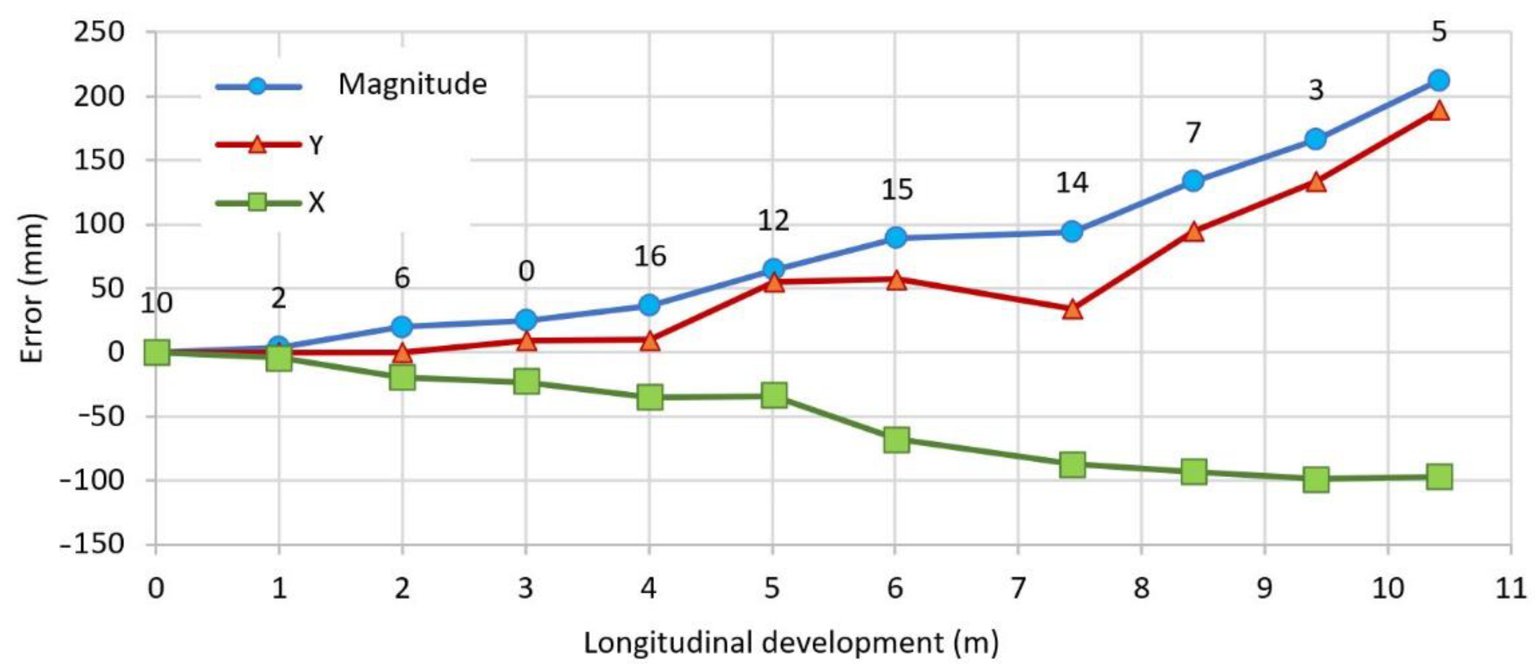
To interpret the error between them, the longest circuit without branches in the test network is reviewed; this corresponds to the sequence of nodes (10, 2, 6, 0, 16, 12, 15, 14, 7, 3, and 5), which is reported in
Table 2. This shows how the distance between the control nodes and those of the map gradually grows, until it reaches a maximum at node 5. This has been graphed as shown in
Figure 13, where three lines correspond to the deltas of the error in the sense of the X and Y axes separately; the magnitude R of the vector is formed by the deltas.
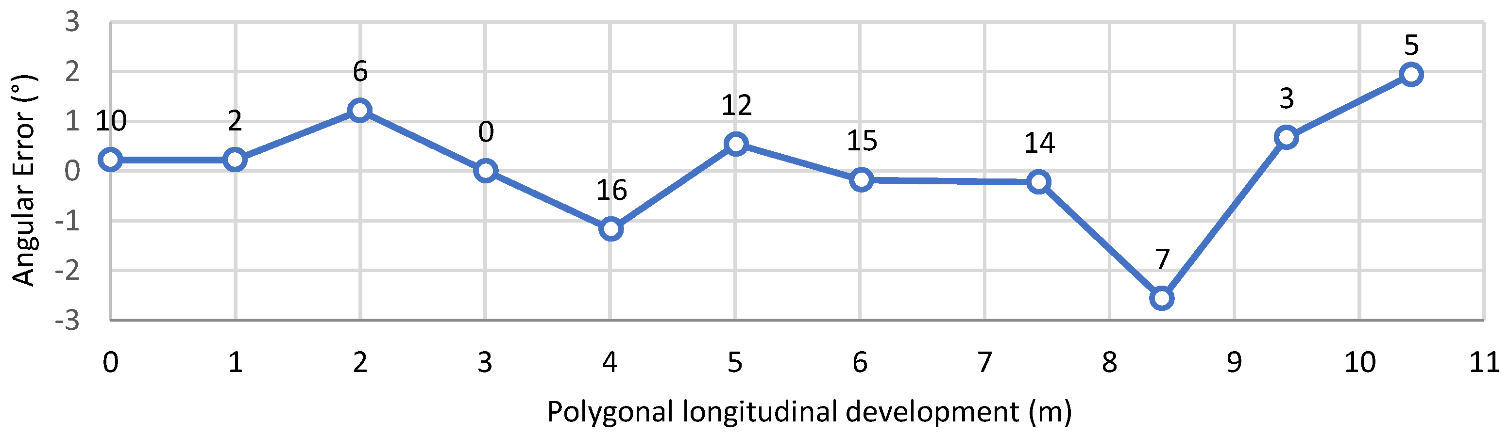
The accumulated longitudinal error in the nodes of the path does not correspond to the angular error defined by the difference between the deflection angles of the control traverse and the map (plotted in
Figure 14), which is notably oscillating because it is not associated to a direct measurement, but rather to a calculation derived from azimuths.
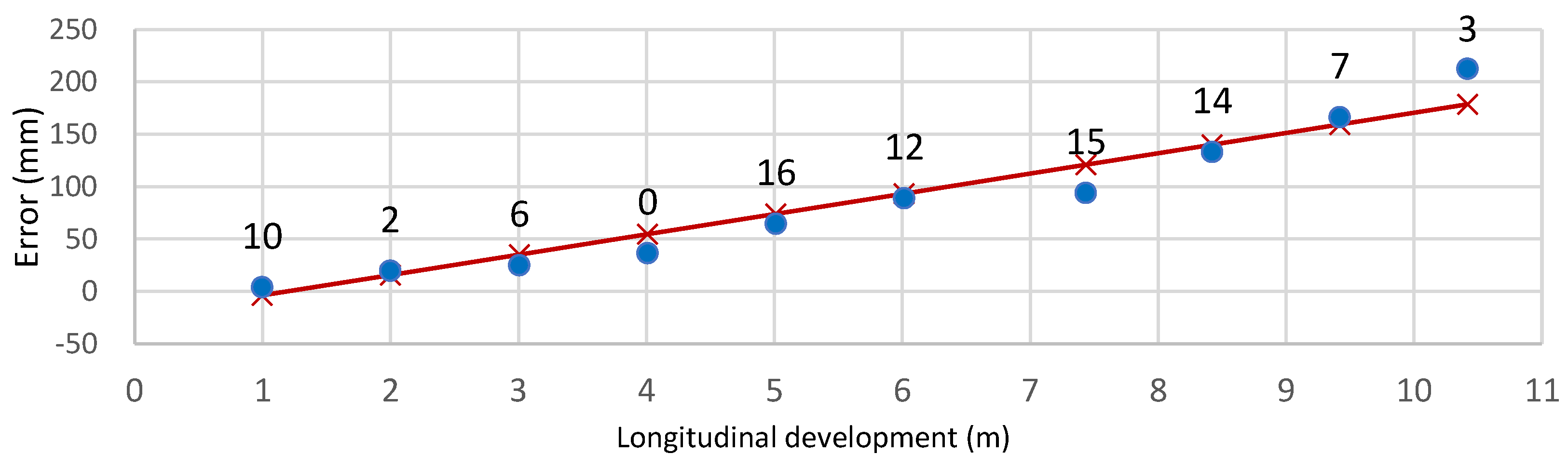
When focusing on the magnitudes of the resulting error of phase shift (R), as shown in
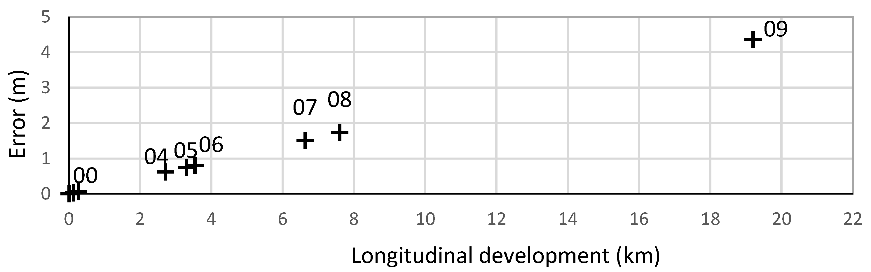
Figure 15, a smooth sinusoidal pattern is noted, where the linear approximation line is the axis, with a slope of 2.3%. If such longitudinal development error is conserved when operating in larger-scale networks, and it is extrapolated based on the length of the longest traverse without derivations, within the nine model networks, the linear magnitudes of the resulting error can be obtained (as shown in
Table 3 and graphed in
Figure 16). This extrapolation has, in parallel, the growth of the ordinary number of operations per station and those derived from the extension of nodes due to exceeding the range of the metrology system.
5. Discussion
Derived from the first network R00 test, with the objective of quantifying the quality of the data produced by comparing a physical network of known dimensions and representative geometry, it is concluded that the offset error against the longitudinal development of the prospecting circuit is cumulative. However, the error rate is substantially linear, with an average value of 2.3%. This error is within acceptable parameters for conventional topography procedures.
As the network test R00 is a limited extension with respect to the average infrastructure networks in the field, the second test was conducted using virtual replicas of real networks of known metropolitan areas; for larger and more complex databases, these tests focused on the performance of the algorithm logic.
The most significant source of error is in the length measurement process, associated with two variables that affect the performance of the IR laser sensor: the light intensity and the range. These two variables can reduce their effects if (a) a sensor is selected whose distance measurement range is higher than the average of the lengths of the edges of the network, in order to reduce the number of operations by repositioning when the range is exceeded, and (b) the laser sensor is calibrated considering the ambient light intensity, whilst also implementing a light intensity sensor on the chassis of the robot units and programming a routine for the operating system to calibrate.
The second significant error derives from the measurement of angles, which is associated with two variables: the sensitivity of the encoder of the azimuth rotation servomotor of the metrology module and the character of the point measurement with the state in the slave robot units as a reference during the collimation procedure. The first effect can be addressed by selecting a servomotor with a higher resolution encoder or by changing the rotation mechanism in direct connection with the arrow of the servomotor (parallel) to a rotational one with dividers (serial) of gears or pulleys, as is often done in radial lidar devices. In the second case, the control loop can include a better PID scheme to position the collimation pointing to the vertical axis of the state, fine-tuning the location sweep cycles.
6. Conclusions
As discussed in the previous section, a navigation system for a group of mobile robots dedicated to the production of maps for underground hydraulic infrastructure was presented. Tarry’s principles of deep search, Pledge modify discrimination, and topographic orientation transfer were used in the temporary construction of a reference network, independent of peripheral inertial navigation.
In future work, for the peripheral navigation, approach operations could be reduced by increasing the number of ultrasonic sensors on the chassis of the robot unit with an octagonal arrangement, which would improve the detection of discontinuities associated with the locations of the nodes. In addition, the redistribution of the hardware components in the robot units could reduce the space occupied by the batteries and reduce the total height, which would allow operation in smaller diameters.
In addition, the algorithm could contemplate one more slave robot unit to increase the redundancy of the triangulation, increasing the sampling of distance and angle measurements to improve the reliability of the results.
Author Contributions
Conceptualization, E.R.; methodology, E.R.; validation, A.V.-M., A.R.S. and Y.A.D.; formal analysis, A.R.S., Y.A.D. and C.H.-S.; investigation, E.R., Y.A.D. and C.H.-S.; resources, E.R.; writing—original draft preparation, E.R. and C.H.-S.; writing—review and editing, A.V.-M., C.H.-S. and Y.A.D.; visualization, A.V.-M., C.H.-S. and A.V.-M. All authors have read and agreed to the published version of the manuscript.
Funding
This research received no external funding.
Institutional Review Board Statement
Not applicable.
Informed Consent Statement
Not applicable.
Data Availability Statement
Not applicable.
Conflicts of Interest
The authors declare no conflict of interest.
References
- Ribera, C.; Ángel, M. Control de Velocidad y Dirección de un Vehículo Terrestre Autónomo; Universidad de Alicante, Departamento de Física, Ingeniería de Sistemas y Teoría de la Señal: Alicante, Spain, 2018. [Google Scholar]
- Wang, C.; Meng, L.; She, S.; Mitchell, I.M.; Li, T. Autonomous mobile robot navigation in uneven and unstructured indoor environments. In Proceedings of the 2017 IEEE/RSJ International Conference on Intelligent Robots and Systems, Vancouver, BC, Canada, 24–28 September 2017; pp. 109–116. [Google Scholar] [CrossRef] [Green Version]
- Kumar, R.; Jitoko, P.; Kumar, S.; Pillay, K.; Prakash, P.; Sagar, A.; Singh, R.; Mehta, U. Maze solving robot with automated obstacle avoidance. In Proceedings of the 2016 IEEE International Symposium on Robotics and Intelligent Sensors, IRIS, Tokyo, Japan, 17–20 December 2016; 2016. [Google Scholar]
- Costa, V.A.; Justo, C.E. El Álgebra Lineal en la Resolución de Problemas Altimétricos de Topografía; U. de la Plata: Buenos Aires, Argentina, 2016; pp. 13–20. [Google Scholar]
- Wolf, P.R.; Ghilani, C.D. Topografía, 14th ed.; Alfaomega: Mexico City, México, 2016; pp. 10, 73, 81, 94, 133, 145–147, 150. [Google Scholar]
- Adamatzky, A. Physical maze solvers, All twelve prototypes implement 1961 Lee algorithm. In Emergent Computation; University of the West of England: Bristol, UK, 2016. [Google Scholar]
- Lösch, R.; Grehl, S.; Donner, M.; Buhl, C.; Jung, B. Design of an autonomous robot for mapping, navigation, and manipulation in underground mines. In Proceedings of the 2018, IEEE/RSJ International Conference on Intelligent Robots and Systems (IROS), Madrid, Spain, 1–5 October 2018; pp. 1407–1412. [Google Scholar]
- Reza, J. Vehicle Dynamics, Theory and Application; Springer: New York, NY, USA, 2017; p. 235. [Google Scholar] [CrossRef]
- Barfoot, T.D.; McManus, C.; Anderson, S.; Dong, H.; Beerepoot, E.; Tong, C.H.; Furgale, P.; Gammell, J.D.; Enright, J. Into Darkness: Visual Navigation Based on a Lidar-Intensity-Image Pipeline. In Robotics Research; Tracts in Advanced Robotics 114; Springer: New York, NY, USA, 2016. [Google Scholar]
- Levin, E.; Nadolinets, L. Surveying Instrumetns and Technology; CRC Press: Boca Raton, FL, USA, 2017; pp. 50–80. [Google Scholar]
- Bienias, Ł.; Szczepański, K.; Duch, P. Maze Exploration Algorithm for Small Mobile Platforms. Image Processing Commun. 2016, 21, 15–26. [Google Scholar] [CrossRef] [Green Version]
- Chand, M.; Goel, M.; Rathore, S. Maze Solving Algorithms. Manish Department of Computer Science; Maharaja Agrasen Institute of Technology G.G.S.I.P.U.: New Delhi, India, 2017. [Google Scholar]
- Velasco, J.; Prieto, J.F.; Herrero, T.R. Metodología de diseño, observación y cálculo de redes geodésicas interiores en túneles de ferrocarril de alta velocidad. Inf. Constr. 2015, 67, 78. [Google Scholar] [CrossRef] [Green Version]
- Salinas González, D.A. Trabajos Topográficos en la Ejecución de Túneles para Carreteras y Ferrocarriles. Ph.D. Thesis, Universitat Politècnica de València, Valencia, Spain, 2017; p. 99. [Google Scholar]
- Patel, Y.D.; George, P.M. Parallel manipulators applications, a survey, modern mechanical engineering. Mod. Mech. Eng. 2012, 2, 57–64. [Google Scholar] [CrossRef] [Green Version]
- Arda, M. Dynamic analysis of a Four-Bar linkage mechanism. Mach. Technol. Mater. 2020, 5, 186–190. [Google Scholar]
- Incerti, G. On the dynamic behavior of a four-bar linkage driven by a velocity-controlled dc motor. Int. J. Mech. Mechatron. Eng. 2012, 6, 1895–1901. [Google Scholar]
- Zhang, Y.X.; Cong, S.; Shang, W.W.; Li, Z.X.; Jiang, S.L. Modeling, identification and control of a redundant planar 2-DOF parallel manipulator. Int. J. Control. Autom. Syst. 2007, 5, 559–569. [Google Scholar]
- Shan, J.; Toth, C.K. (Eds.) Topographic Laser Ranging and Scanning, Principles and Processing, 2nd ed.; CRC Press: Boca Raton, FL, USA, 2018. [Google Scholar]
- Schittter, G. Advanced Mechatronics for Precision Engineering and Mechatronic Imaging Systems. IFAC-PapersOnLine 2015, 48, 942–943. [Google Scholar] [CrossRef]
- Singh, A.; Sachdeva, E.; Sarkar, A.; Krishna, K.M. Compliant Omni-Crawler In-Pipeline Robot. In Proceedings of the 2017 IEEE/RSJ International Conference on Intelligent Robots and Systems, Vancouver, BC, Canada, 24–28 September 2017. [Google Scholar] [CrossRef] [Green Version]
- Ahmed, W.; Amer, R.A.; Fatima, S. Steering strategy for a multi-axle wheeled vehicle. In Proceedings of the ASME 2018, International Mechanical Engineering Congress and Exposition, IMECE2018-86323, Pittsburgh, PA, USA, 9–15 November 2018. [Google Scholar]
Figure 1.
(a) Mechanical design of the chassis of the robot units, compatible with Broadcom and ATmega 2560 cards, in the left section of the chassis; (b) Lateral view; (c) Frontal view.
Figure 1.
(a) Mechanical design of the chassis of the robot units, compatible with Broadcom and ATmega 2560 cards, in the left section of the chassis; (b) Lateral view; (c) Frontal view.
Figure 2.
Master (E0) and slave (Ei) robot unit inside a 12” diameter duct.
Figure 2.
Master (E0) and slave (Ei) robot unit inside a 12” diameter duct.
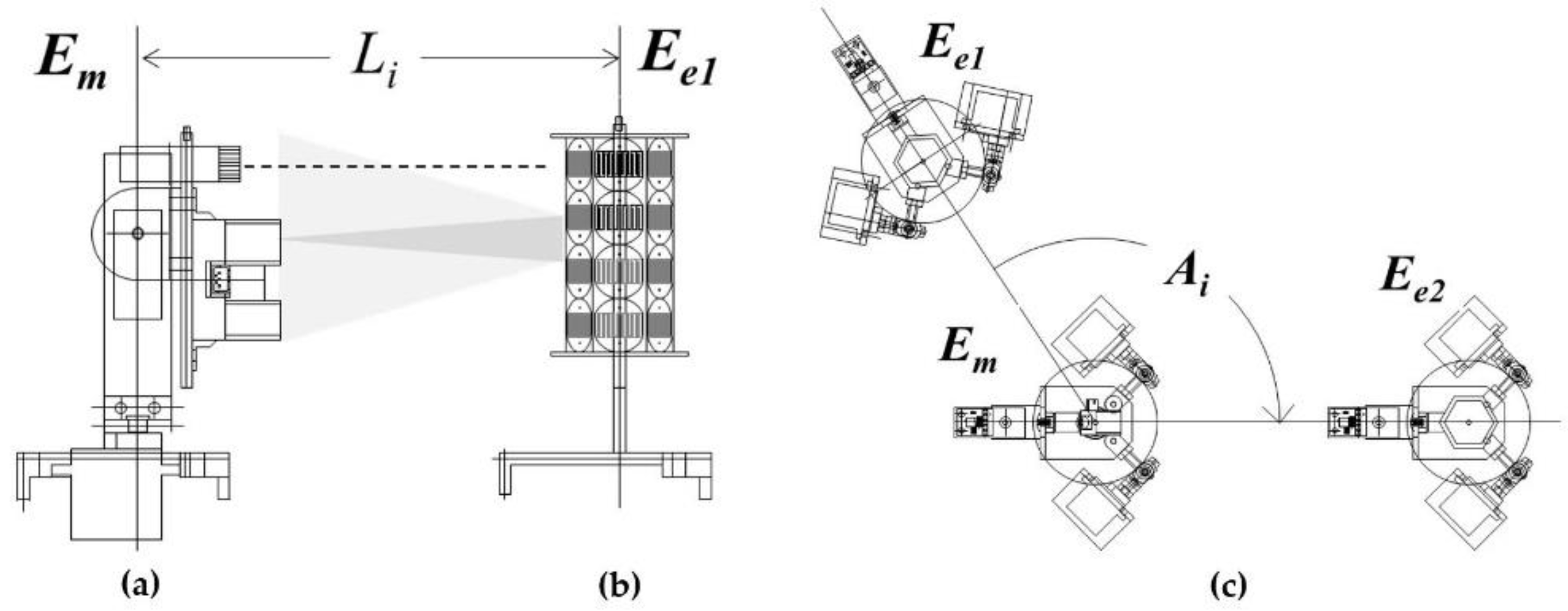
Figure 3.
Metrology system. (a) Collimating emitter; (b) Receiving rod; (c) Arrangement for measuring an azimuth angle.
Figure 3.
Metrology system. (a) Collimating emitter; (b) Receiving rod; (c) Arrangement for measuring an azimuth angle.
Figure 4.
(a) Robot kinematic chains; (b) Self-leveling platform kinematic chain; (c) Mechanical implementation.
Figure 4.
(a) Robot kinematic chains; (b) Self-leveling platform kinematic chain; (c) Mechanical implementation.
Figure 5.
Kinematic chain using θ4 as input, with θ1 as output.
Figure 5.
Kinematic chain using θ4 as input, with θ1 as output.
Figure 6.
Target acquisition cycle.
Figure 6.
Target acquisition cycle.
Figure 7.
Mapping process and data-processing approach.
Figure 7.
Mapping process and data-processing approach.
Figure 8.
Diagram of the SPI network of the robot units.
Figure 8.
Diagram of the SPI network of the robot units.
Figure 9.
(a) Diagram of the network R00; (b) Triangular control mesh for the plot; (c) Graph of the test network.
Figure 9.
(a) Diagram of the network R00; (b) Triangular control mesh for the plot; (c) Graph of the test network.
Figure 10.
Sequence of the development of the Network 00 for the validation of the navigation algorithm.
Figure 10.
Sequence of the development of the Network 00 for the validation of the navigation algorithm.
Figure 11.
Extensive test networks for the validation of the navigation algorithm.
Figure 11.
Extensive test networks for the validation of the navigation algorithm.
Figure 12.
Node geometric offset error, control mesh versus mapping system.
Figure 12.
Node geometric offset error, control mesh versus mapping system.
Figure 13.
Geometric offset error of nodes, axial (X and Y) and magnitude (R).
Figure 13.
Geometric offset error of nodes, axial (X and Y) and magnitude (R).
Figure 14.
Angular error at the vertices of the longest traverse without islands.
Figure 14.
Angular error at the vertices of the longest traverse without islands.
Figure 15.
Magnitude node geometric offset error (R), linear approximation.
Figure 15.
Magnitude node geometric offset error (R), linear approximation.
Figure 16.
Extrapolation of the lag error to larger network models.
Figure 16.
Extrapolation of the lag error to larger network models.
Table 1.
Elements of the CPT node vector.
Table 1.
Elements of the CPT node vector.
| i | Node | i | Node | i | Node | i | Node | i | Node |
|---|
| 1 | 0 | 9 | 8 | 17 | 5 | 25 | 4 | 33 | 15 |
| 2 | 1 | 10 | 9 | 18 | 3 | 26 | 5 | 34 | 16 |
| 3 | 2 | 11 | 10 | 19 | 12 | 27 | 6 | 35 | 17 |
| 4 | 3 | 12 | 9 | 20 | 13 | 28 | 7 | 36 | 16 |
| 5 | 4 | 13 | 8 | 21 | 12 | 29 | 5 | 37 | 15 |
| 6 | 5 | 14 | 11 | 22 | 14 | 30 | 3 | 38 | 1 |
| 7 | 6 | 15 | 8 | 23 | 12 | 31 | 2 | 39 | 0 |
| 8 | 7 | 16 | 7 | 24 | 3 | 32 | 1 | | |
Table 2.
Geometric offset error of nodes, axial (X and Y) and magnitude (R).
Table 2.
Geometric offset error of nodes, axial (X and Y) and magnitude (R).
| Node | Control | Map | Longitudinal
Development (m) | Error |
|---|
| Axial | Magnitude |
|---|
| X | Y | X | Y | X | Y | R |
|---|
| 10 | 414.9 | 0.0 | 414.9 | 0.0 | 0 | 0.00 | 0.00 | 0.00 |
| 2 | 1415.8 | 0.0 | 1411.8 | 0.0 | 996.90 | −4.00 | 0.00 | 4.00 |
| 6 | 1415.8 | 1000.6 | 1396.1 | 1000.5 | 1997.50 | −19.72 | −0.12 | 19.72 |
| 0 | 2416.4 | 0.0 | 2408.4 | 3.1 | 3007.13 | −23.28 | 9.04 | 24.97 |
| 16 | 708.3 | 2709.2 | 673.2 | 2719.2 | 4009.13 | −35.08 | 9.97 | 36.47 |
| 12 | 1708.9 | 2709.2 | 1674.8 | 2764.0 | 5011.73 | −34.09 | 54.84 | 64.57 |
| 15 | 1708.9 | 3710.0 | 1640.9 | 3767.3 | 6015.53 | −67.98 | 57.27 | 88.89 |
| 14 | 2709.7 | 2709.2 | 2622.2 | 2743.4 | 7433.71 | −87.47 | 34.23 | 93.93 |
| 7 | 2709.7 | 1711.9 | 2616.4 | 1806.8 | 8421.31 | −93.27 | 94.93 | 133.08 |
| 3 | 1998.3 | 1001.2 | 1899.3 | 1134.7 | 9418.85 | −98.95 | 133.48 | 166.16 |
| 5 | 1290.6 | 1708.1 | 1193.5 | 1897.2 | 10,418.12 | −97.08 | 189.11 | 212.57 |
Table 3.
Geometric offset error, extrapolation to larger networks.
Table 3.
Geometric offset error, extrapolation to larger networks.
| Network | Sections | Nodes | Development
Longitudinal (m) | Operations | Error |
|---|
| Total | Path | Total | Path | Total | Path | Total | Path | (m) |
|---|
| 00 | 19 | 10 | 18 | 11 | 19.8 | 10.4 | 114 | 60 | 0.2 |
| 01 | 34 | 21 | 31 | 22 | 35.8 | 17.9 | 204 | 126 | 0.4 |
| 02 | 117 | 42 | 96 | 43 | 21,183.0 | 7604.1 | 702 | 252 | 172.7 |
| 03 | 600 | 70 | 355 | 71 | 30,336.7 | 3539.3 | 3600 | 420 | 80.4 |
| 04 | 591 | 47 | 390 | 48 | 241,476.6 | 19,203.7 | 3546 | 282 | 436.1 |
| 05 | 730 | 70 | 511 | 71 | 69,181.4 | 6633.8 | 4380 | 420 | 150.6 |
| 06 | 98 | 38 | 118 | 39 | 8518.1 | 3302.9 | 588 | 228 | 75.0 |
| 07 | 264 | 46 | 220 | 47 | 1536.4 | 267.7 | 1584 | 276 | 6.1 |
| 08 | 493 | 38 | 226 | 39 | 1786.2 | 137.7 | 2958 | 228 | 3.1 |
| 09 | 597 | 92 | 575 | 93 | 17,592.1 | 2711.0 | 3582 | 552 | 61.6 |
| Publisher’s Note: MDPI stays neutral with regard to jurisdictional claims in published maps and institutional affiliations. |
© 2022 by the authors. Licensee MDPI, Basel, Switzerland. This article is an open access article distributed under the terms and conditions of the Creative Commons Attribution (CC BY) license (https://creativecommons.org/licenses/by/4.0/).


 ,
, 


