An Improved Convolutional-Neural-Network-Based Fault Diagnosis Method for the Rotor–Journal Bearings System

Abstract

More layers in a convolution neural network (CNN) means more computational burden and longer training time, resulting in poor performance of pattern recognition. In this work, a simplified global information fusion convolution neural network (SGIF-CNN) is proposed to improve computational efficiency and diagnostic accuracy. In the improved CNN architecture, the feature maps of all the convolutional and pooling layers are globally convoluted into a corresponding one-dimensional feature sequence, and then all the feature sequences are concatenated into the fully connected layer. On this basis, this paper further proposes a novel fault diagnosis method for a rotor–journal bearing system based on SGIF-CNN. Firstly, the time-frequency distributions of samples are obtained using the Adaptive Optimal-Kernel Time–Frequency Representation algorithm (AOK-TFR). Secondly, the time–frequency diagrams of the training samples are utilized to train the SGIF-CNN model using a shallow information fusion method, and the trained SGIF-CNN model can be tested using the time–frequency diagrams of the testing samples. Finally, the trained SGIF-CNN model is transplanted to the equipment’s online monitoring system to monitor the equipment’s operating conditions in real time. The proposed method is verified using the data from a rotor test rig and an ultra-scale air separator, and the analysis results show that the proposed SGIF-CNN improves the computing efficiency compared to the traditional CNN while ensuring the accuracy of the fault diagnosis.

1. Introduction

Hydrodynamic journal bearings, as one of the main mechanical moving parts of rotating machinery, always remain prone to failure because of the harsh industrial environment and no doubt display increasing probability of failure with service life. As such, effective maintenance for rotor–journal bearing systems is necessary to ensure that these machines can be operated properly. Conventional maintenance techniques for rotor–journal bearing systems can be broadly classified into three categories [1]: breakdown maintenance (BM), scheduled maintenance (SM) and condition-based maintenance (CBM). SM sets a periodic interval to perform overhauling regardless of the health status of a machine, while BM takes place when failure has already occurred. Unfortunately, due to the increasing complexity and the better quality and reliability requirements of rotating machinery, both methods have a substantial economic impact and potential safety concerns, rendering them unsuitable for complex industrial machines. In comparison, CBM is a better choice for complex rotating machinery, as it attempts to avoid unnecessary maintenance tasks by taking maintenance actions only when there is evidence of abnormal behavior of the machines [2]. Implementing a CBM paradigm requires the machine’s health to be monitored in a timely and accurate manner. Therefore, condition monitoring and fault diagnostics of rotor–journal bearing systems are gaining heightened popularity.

During the service life of rotor–journal bearings systems, the potential failure modes can be classified as characteristic faults (due to oil film instability), which occur only in oil-film-bearing-supported rotor systems, or common faults (due to imbalance, misalignment, cracked shaft, excessive preload, loose rotating part and rub), which can occur in all rotating machinery [3,4]. Conventional fault diagnosis techniques for rotor–journal bearing systems can be classified into two categories [5]: traditional signal-processing techniques and machine learning techniques.

Identifying the fault types of rotor–journal bearing systems using the various signal-processing-technique-based methods is a time-consuming and laborious work which requires a certain amount of prior knowledge [6] and cannot meet the real-time requirements imposed by CBM. Compared with the traditional signal-processing-technique-based methods, machine-learning-based intelligent diagnosis methods can automatically handle the vibration data and comprehensively recognize fault patterns of rotating machinery.

Generally, there are two types of machine-learning-based fault diagnosis techniques: traditional machine learning techniques and deep learning techniques. The traditional machine learning algorithms commonly applied in intelligent fault diagnosis of rotating machinery mainly contain support vector machines (SVM) [7,8] and artificial neural networks (ANN) [9,10]. However, the traditional intelligent diagnosis methods have inherent limitations [11]: (1) Variable working conditions and composite faults make it difficult to extract signal features effectively; (2) the extracted signal features must be selected with the advice of experienced engineering experts; (3) shallow machine learning algorithms are not able to adequately learn complex nonlinear relationships between the input data.

The deep-learning-based fault diagnosis approach for rotating machinery can learn the raw input’s deep-level representations and hierarchical patterns, providing significant improvements in generalization capability and classification accuracy. Deep learning architectures such as deep belief networks [12], deep autoencoder networks [13], recurrent neural networks [14,15] and convolution neural networks (CNN) [16,17,18] have been applied to the field of failure diagnosis of rotation machinery. Among them, the CNN-based intelligent fault diagnosis methods have the capability of representation learning, which can effectively learn the in-depth information of the raw input in a shift-invariant manner and have achieved some results in the fault diagnosis of rotor–journal bearing systems. Alves et al. [19] proposed a CNN-based condition monitoring method for the rotor–journal bearings to predict ovalization faults in hydrodynamic journal bearings. Using shaft orbit images generated from vibration signals, Jiang et al. [20] proposed a multilayer CNN model to diagnose the faults of turbomachines, improving the generality and robustness of the CNN. Shao et al. [21] developed an enhanced CNN-based fault diagnosis method to detect the faults of a rotor–bearing system under variable operating conditions. He et al. [22] proposed a CNN-based fault diagnosis method for the rotor-bearing systems using small labeled infrared thermal images as model input. Kumar et al. [23] proposed a sparse CNN-based fault diagnosis for rotor–bearing systems at varying speeds by developing sparsity cost in the existing cost function of a CNN to enhance the learning capability of the CNN.

Although the CNN-based fault diagnosis method has academically achieved certain results in fault diagnosis of rotor–journal bearing systems, diagnostic performance still needs to be improved to meet the challenges of the complex industrial production scene. Harsh industrial environments place high accuracy and time requirements on equipment condition monitoring systems. The common approach to improve CNN accuracy is increasing the network’s depth and width. However, more layers and kernels in the CNN architecture imply more computational burden and longer training time. The parameter size of a CNN model can reach hundreds of thousands or even millions, leading to overfitting, vanishing gradient, and low computational efficiency. Therefore, improving the accuracy of CNN models without significantly increasing the amount of computation is a difficult problem for industrial applications of CNN-based fault diagnosis methods. In addition, only the last pooling layer’s feature maps are input into the fully connected layer, and the feature maps of the shallow layers are all neglected in the typical CNN structures. Therefore, it is of practical value to improve the performance of fault diagnosis methods based on CNNs by integrating the shallow information while reducing the parameter size of the model.

To address the issues mentioned above, some researchers have adopted various methods to improve the pattern recognition performance of CNNs. Lin et al. [24] proposed a novel CNN structure called “Network In Network” to enhance model discriminability by stacking three multilayer perceptron convolutional layers and one global average pooling layer. Wu et al. [25] proposed a CNN-based automatic modulation classification method with multi-feature fusion, and experimental results show that the proposed method has good performance on the public dataset. Li et al. [26] proposed a modified CNN for fault diagnosis based on the LeNet-5 architecture by replacing the fully connected layer with a global average pooling layer. Wang et al. [27] proposed an end-to-end health state diagnostics model based on a CNN with multiscale feature extraction modules, which can directly learn feature maps from the raw vibration signal. Kim et al. [28] propose a direct-connection-CNN-based fault diagnosis method for rotor systems by improving the connectivity between various layers within the CNN. Kumar et al. [29] proposed a CNN model with multiple convolutional layers and batch normalization layers to detect the bearing faults in a squirrel cage induction motor. Wang et al. [30] proposed an improved 1D-CNN-based bearing fault diagnosis method by processing long-time series by introducing a dilated convolution operation. Zhang et al. [31] proposed an improved CNN model with multiscale feature extraction to diagnose bearing defects using limited training samples. Luo et al. [32] proposed an improved CNN framework with shallow pooling layer information fusion to detect the faults of high-speed train axle–box bearing systems. Fu et al. [33] proposed a residual-learning-based CNN with multiscale comprehensive feature fusion to recognize vehicle color. Jun et al. [34] proposed an improved CNN model with multilayer information fusion to predict the remaining useful life of bearings. Sang et al. [35] presented an improved CNN model with a multi-information flow for person reidentification. Nguyen et al. [36] constructed a multibranch structure deep neural network model to diagnose bearing faults using multiple-domain image representation data.

However, as the improved CNN models mentioned above input information from the shallow layers to the classification layer, the parameter sizes in these CNN models are large, and the required memory tends to increase very quickly with high hardware resource consumption. The performance of these methods mentioned above still must be improved to meet the challenge of complex industrial scenarios. In this work, a simplified global information fusion-CNN (SGIF-CNN) model is presented to enhance the performance of the CNN-based fault diagnosis approach for rotor–journal bearing systems without increasing computational burden. In the SGIF-CNN structure, the feature maps of all the convolutional and pooling layers are globally convolved into a corresponding feature sequence. Then, all the feature sequences are concatenated into a one-dimensional feature vector before connecting to the fully connected layer for the pattern recognition task. The effectiveness of the SGIF-CNN-based fault diagnosis approach for rotor–journal bearing systems is evaluated on experimental datasets from a test bench and engineering datasets from an ultralarge air separator. The results of case studies on datasets of the rotor–journal bearing systems show that the SGIF-CNN model could improve computing efficiency and fault diagnosis accuracy compared to a traditional CNN.

The main contributions of this paper are summarized as follows:

(1)

A novel SGIF-CNN architecture is proposed to reduce model parameter size and enhance network capacity by shortcutting the simplified information of the shallow layers.

(2)

Time–frequency plots with an excellent resolution of the vibration data acquired from the rotor–journal bearing system are generated using the Adaptive Optimal Kernel Time–Frequency Representation (AOK-TFR) algorithm. As a result, proper features for different health conditions of the rotor–journal bearing systems can be obtained.

(3)

A novel fault diagnosis method for rotor–journal bearing systems based on AOK-TFR and SGIF-CNN is proposed. By concatenating the simplified shallow layers’ information into the fully connected layer, the effective information amount input into the classification layer can be increased without increasing computational burden.

(4)

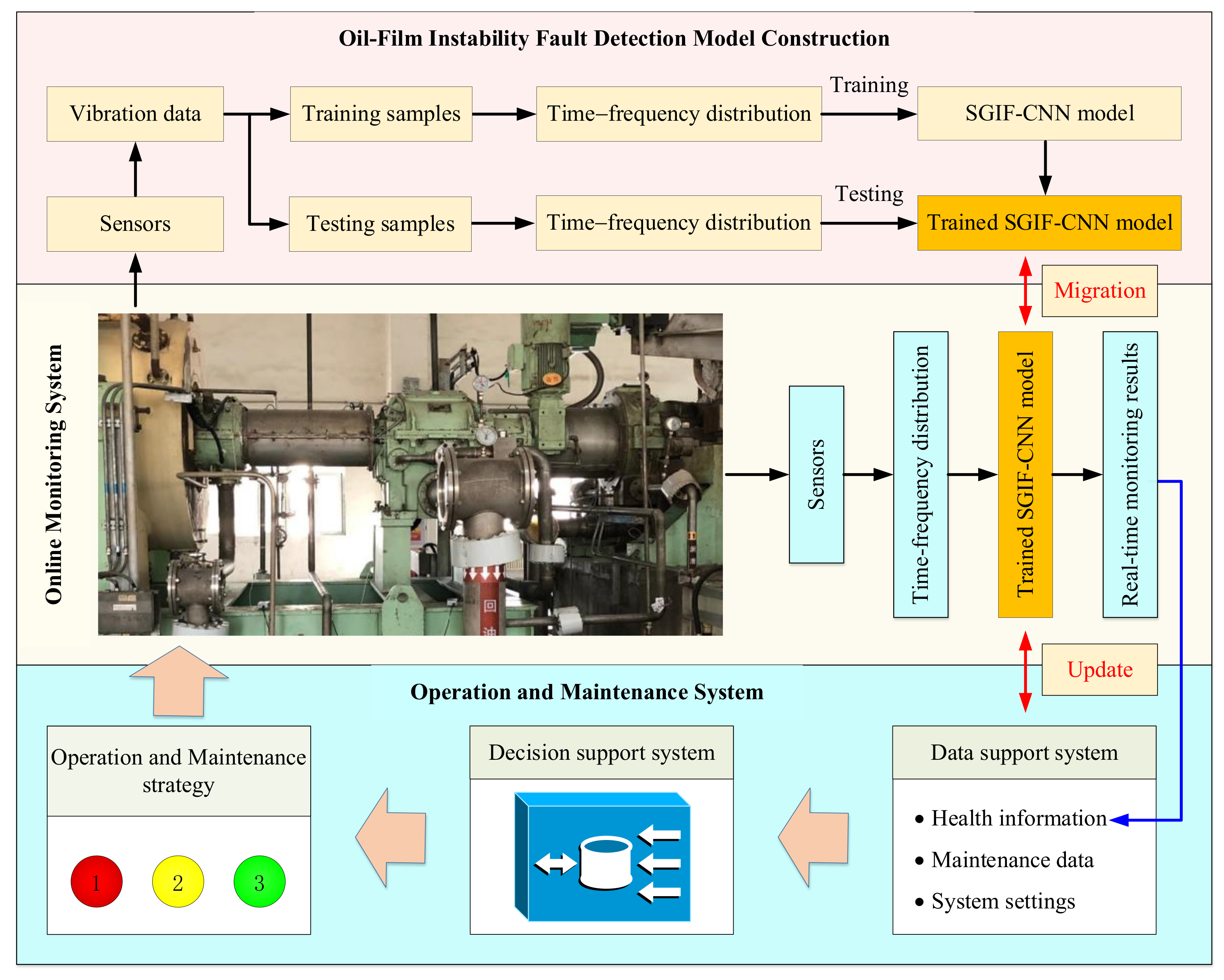
The industrial applications framework of the SGIF-CNN-based fault diagnosis method for rotor–bearing systems is presented to realize the real-time fault monitoring of the ultralarge air separator in a production plant.

The remainder of this paper is organized as follows. Section 2 provides a brief review of AOK-TFR and CNN. In Section 3, the principle of SGIF-CNN and the methodology of the fault diagnosis method based on AOK-TFR and SGIF-CNN are presented. In Section 4, validations of the proposed method with experimental and engineering datasets are presented and discussed. Finally, some conclusions are drawn in Section 5.

2. Theoretical Background

2.1. Wigner–Ville Distribution

The Wigner–Ville distribution (WVD) can extract the joint distribution information of nonstationary signals in the time and frequency domain with an excellent resolution. For a square-integrable signal $x\left(t\right)$, its Wigner–Ville distribution can be defined as:

$$WV{D}_x\left(t,f\right)={{\displaystyle \int }}_{-\infty }^{\infty }x\left(t+\frac{\tau }{2}\right)x^{*}\left(t-\frac{\tau }{2}\right)e^{-j2\pi f\tau }d\tau$$

(1)

where $x^{*}\left(t\right)$ is the conjugate of $x\left(t\right)$, and $j$ is the imaginary unit. The integrand function $x\left(t+\frac{\tau }{2}\right)x^{*}\left(t-\frac{\tau }{2}\right)$ is defined as the Wigner autocorrelation function $K_x\left(t,\tau \right)$, and the WVD can be viewed as the Fourier transform of the function $K_x\left(t,\tau \right)$ to the time delay $\tau$. If the inverse Fourier transform is performed for time $t$, the ambiguity function is given by:

$$A_x\left(\tau ,\upsilon \right)={{\displaystyle \int }}_{-\infty }^{\infty }x\left(t+\frac{\tau }{2}\right)x^{*}\left(t-\frac{\tau }{2}\right)e^{j2\pi \upsilon t}dt$$

(2)

The Wigner–Ville distribution can be derived from a two-dimensional Fourier transform of $A_x\left(\tau ,\upsilon \right)$ function:

$$WV{D}_x\left(t,f\right)=\iint A_x\left(\tau ,\upsilon \right)e^{-j2\pi \left(t\upsilon +\tau f\right)}d\upsilon d\tau$$

(3)

The WVD has a good time–frequency localization property, but for the multicomponent signals $x\left(t\right)={\displaystyle {\displaystyle \sum }_i}{x}_i\left(t\right)$, the Wegener autocorrelation function is:

$$\begin{array}{cc}\hfill K_x\left(t,\tau \right)& =\left({\displaystyle {\displaystyle \sum }_i}{x}_i\left(t+\frac{\tau }{2}\right)\right)·\left({\displaystyle {\displaystyle \sum }_i}{x}_i\left(t-\frac{\tau }{2}\right)\right)\hfill \\ \hfill & ={\displaystyle {\displaystyle \sum }_i}{x}_i\left(t+\frac{\tau }{2}\right)·x_i^{*}\left(t-\frac{\tau }{2}\right)+{\displaystyle {\displaystyle \sum }_i}{\displaystyle {\displaystyle \sum }_j}{x}_i\left(t+\frac{\tau }{2}\right)·x_j^{*}{\left.\left(t-\frac{\tau }{2}\right)\right|}_{i\ne j}\hfill \\ \hfill & =K_a\left(t,\tau \right)+K_c\left(t,\tau \right)\hfill \end{array}$$

(4)

where $K_a\left(t,\tau \right)$ is autocorrelation component of interest, and $K_c\left(t,\tau \right)$ is the intercorrelation component that causes interference, i.e., the “cross term” problem. Suppressing the cross term generated by the Wigner–Ville distribution is one of the key problems studied by scholars.

2.2. Adaptive Optimal-Kernel Time–Frequency Representation

Linear transforms such as the short-time Fourier transform (STFT) and wavelet transform (WT) are subject to the Heisenberg uncertainty principle for their time–frequency resolution due to the effect of the window function. The WVD has no windowing operation, and the product of the time domain and frequency bandwidth reaches the lower bound of the Heisenberg principle. The time–frequency localization performance of WVD is more desirable, but its application is more limited due to the cross-interference term problem, which is a common problem in quadratic algorithms. To suppress the cross-terms and obtain the time–frequency resolution of the Wigner–Ville distribution, Jones et al. [37] proposed a signal-dependent adaptive kernel time–frequency analysis method in which the kernel function can be adaptively adjusted according to the signal characteristics. The signal-dependent kernel function is called as a 2D radially Gaussian function:

$$\varphi \left(\tau ,\upsilon \right)=\exp \left(-\frac{{\tau }^2+{\upsilon }^2}{2{\sigma }^2\left(\theta \right)}\right)$$

(5)

where $\sigma \left(\theta \right)$ is the variance of the Gaussian function along the radial angle $\theta =arctan\left(\tau /\upsilon \right)$.

Then, the optimal kernel function $\varphi \left(\tau ,\upsilon \right)$ can be obtained by optimizing the following problem:

$${\max }_{\theta }{{\displaystyle \int }}_0^{2\pi }{{\displaystyle \int }}_0^{+\infty }{\left|A\left(r,\theta \right)\varphi \left(\tau ,\upsilon \right)\right|}^{2}rdrd\theta$$

(6)

subject to

$$\frac{1}{2\pi }{{\displaystyle \int }}_0^{2\pi }{{\displaystyle \int }}_0^{+\infty }{\left|A\left(r,\theta \right)\varphi \left(\tau ,\upsilon \right)\right|}^{2}rdrd\theta \le c,c\ge 0$$

(7)

where $A\left(r,\theta \right)$ is the polar coordinate representation of the ambiguity function, $r=\sqrt{{\tau }^2+{\upsilon }^2}$, and c is the volume of the Gaussian kernel function. Equation (6) restricts the scope of the optimization problem to the Gaussian radial kernels, and Equation (7) restricts the volume of the optimal kernel. The optimal kernel can be regarded as a low pass filter that keeps the auto-terms and suppresses the cross-terms in the time–frequency diagram. The adaptive optimal kernel time–frequency representation (AOK-TFR) can be obtained by using the solved adaptive optimal kernel function:

$${\mathrm{TFR}}_{AOK}\left(t,f\right)=\frac{1}{2\pi }\iint A_x\left(\tau ,\upsilon \right)\varphi \left(\tau ,\upsilon \right)e^{-j2\pi \left(t\upsilon +\tau f\right)}d\upsilon d\tau$$

(8)

2.3. Basic Principle of Convolutional Neural Network

A classical CNN architecture usually consists of three parts: convolutional layers, pooling layers, and a fully connected layer, as shown in Figure 1. A convolutional layer usually contains a set of convolution kernels and one trainable bias per feature map. After the convolutional layer, a pooling layer is usually added between the convolutional layers to merge the outputs of the previous convolutional layer into a single neuron. The feature maps from the last pooling layer will be connected to a fully connected structure after being concatenated into a one-dimensional vector. The fully connected structure may contain one or more hidden layers. A SoftMax layer is usually posted as the output layer to realize the classification tasks by mapping the values of the fully connected layer into a probability distribution that ranges from 0 to 1. Detailed information about convolutional neural networks can be found in [16,18].

3. Methodology

3.1. Global Pooling Information Fusion CNN

In a traditional CNN architecture, the feature maps of shallow layers are neglected, and the confidential information of the raw input with different depths is lost. To increase the amount of information input to the fully connected layer, the feature maps from all the pooling layers are directly concatenated to the fully connected layer to achieve different tasks, as shown in Figure 2.

Compared with a classical CNN structure, the global pooling information fusion CNN (GPIF-CNN) takes account of the shallow pooling information, and the calculations performed by a neuron in the fully connected layer can be expressed as:

$$fc=f\left({\displaystyle \sum }_{m=1}^M{\omega }_m*\left({\displaystyle \sum }_{l=1}^L{P}^l\right)+b_m\right)$$

(9)

where $P^l$ is the set of the output feature maps of lth pooling layer, ${\omega }_m$ is the weight vector and $b_m$ is the bias value of the $m\mathrm{th}$ neuron, M is the number of neurons, and L is the number of pooling layers. It can be noted that the GPIF-CNN contains more neurons in the fully connected layer due to shallow feature maps concatenation and has a larger parameter size, resulting in more computational burden and longer training time.

3.2. Simplified Global Information Fusion-CNN

To reduce parameter size without reducing the amount of input information, the feature maps from all the convolutional and pooling layers are merged into a feature sequence through the corresponding global convolution layers before being concatenated to the fully connected layer to achieve different tasks, as shown in Figure 3.

In the simplified global information fusion-CNN (SGIF-CNN) model, the global convolution kernels have the same dimension as the feature maps from the corresponding convolutional or pooling layer. As shown in Figure 4, the feature sequences extracted from the shallow layers are further concatenated into the fully connected layer. The rectangles with different colors in Figure 4 represent feature vectors outputted by different global convolution kernels, and the circles with different colors represent different neurons. The global convolution kernels are used to convolve the feature maps from layer C₁, and the result G₁ is a feature sequence with a dimension consistent with the number of the feature maps from the convolutional layer C₁. The global convolution features obtained from all the convolutional and pooling layers are concatenated before being inputted into the fully connected layer to achieve different tasks.

The calculations performed by a neuron in the fully connected layer can be expressed as:

$$fc=f\left({\displaystyle \sum }_{m=1}^M{\omega }_m*\left({\displaystyle \sum }_{l=1}^L{\displaystyle \sum }_{k=1}^K(C_k^l⨂G_k^l+P_k^l⨂{\tilde{G}}_k^l)\right)+b_m\right)$$

(10)

where $C_k^l$ is the kth feature map of lth convolutional layer, $G_k^l$ is the global convolution kernel with the same dimension as $C_k^l$, $P_k^l$ is the kth feature map of lth pooling layer, ${\tilde{G}}_k^l$ is the global convolution kernel with the same dimension as $P_k^l$, ${\omega }_m$ is the weight vector and $b_m$ is the bias value of the $m\mathrm{th}$ neuron, M is the number of neurons, and L is the number of conv–pool blocks.

Parameter simplification can be achieved by replacing the feature map with a feature value, and different maps can obtain different convolution information due to the special structure of the global convolution kernel. Therefore, the global convolution kernel has a better classification performance for different feature maps. Replacing the feature maps with a feature sequence will not reduce the amount of original data information but can achieve the purpose of parameter simplification.

3.3. The Proposed Fault Diagnosis Method for the Rotor–Journal Bearing System

The time–frequency representations of the rotor–journal bearing system can reflect its fault information well, and the fault diagnosis can be achieved by inputting the AOK time–frequency images into the SGIF-CNN model. As shown in Figure 5, the proposed method’s modeling procedure follows data acquisition, time–frequency representation extraction, and deep learning model training and testing.

(1)

Dataset generation. The data acquisition system collects the vibration signals of the rotor–journal bearing system under different health conditions using the vibration sensors. The collected vibration data is divided into training and testing datasets according to the corresponding fault patterns.

(2)

Time–frequency image generation. The adaptive kernel time–frequency analysis is performed on each data sample to extract the corresponding time–frequency images.

(3)

Diagnosis model training. The normalized time–frequency images of the training sample are input into the SGIF-CNN designed in Section 3.2 to train the fault diagnosis model. The model is adjusted using the error backpropagation method, and model training can be completed when the error function converges.

(4)

Diagnosis model testing. The time–frequency maps of the testing samples are input into the pretrained fault diagnosis model based on the SGIF-CNN to realize the fault diagnosis of the rotor–journal bearings system.

With a practicable Gaussian kernel volume, the AOK time–frequency images of the sample sets can be obtained effectively before being reshaped to the required size of the input layer of the SGIF-CNN. The mean square error is chosen as the loss function, and the network parameters can be optimized by using the stochastic gradient descent method. The model training ends when the network converges or reaches the specified iteration termination condition.

The architecture designs of the three CNN models—general CNN, GPIF-CNN, and SGIF-CNN—are shown in

Table 1. T The structure design of the general CNN.

Layer	Parameter Setting	Output Size	Activation Function
Input layer	-	3@128 × 128	-
C1	64@5 × 5 kernels, stride: 1 × 1	64@124 × 124	ReLU
P1	2 × 2 max pool, stride: 2 × 2	64@62 × 62	ReLU
C2	128@3 × 3 kernels, stride: 1 × 1	128@60 × 60	ReLU
P2	2 × 2 max pool, stride: 2 × 2	128@30 × 30	ReLU
C3	256@3 × 3 kernels, stride: 1 × 1	256@28 × 28	ReLU
P3	2 × 2 max pool, stride: 2 × 2	256@14 × 14	ReLU
C4	512@3 × 3 kernels, stride: 1 × 1	512@12 × 12	ReLU
P4	2 × 2 max pool, stride: 2 × 2	512@6 × 6	ReLU
Fully connected layer	18,432 neurons	1 × 18,432	ReLU
Classifier hidden layer	1024 neurons	1 × 1024	ReLU
Classification layer	n neurons	1 × n	sigmoid

Note: C and P denote the convolutional layer and the pooling layer, respectively. n is the number of rotor–journal bearing system faults.

,

Table 2. T The structure design of the general CNN.

Layer	Parameter Setting	Output Size	Activation Function
Input layer	-	3@128 × 128	-
C1	64@5 × 5 kernels, stride: 1 × 1	64@124 × 124	ReLU
P1	2 × 2 max pool, stride: 2 × 2	64@62 × 62	ReLU
C2	128@3 × 3 kernels, stride: 1 × 1	128@60 × 60	ReLU
P2	2 × 2 max pool, stride: 2 × 2	128@30 × 30	ReLU
C3	256@3 × 3 kernels, stride: 1 × 1	256@28 × 28	ReLU
P3	2 × 2 max pool, stride: 2 × 2	256@14 × 14	ReLU
C4	512@3 × 3 kernels, stride: 1 × 1	512@12 × 12	ReLU
P4	2 × 2 max pool, stride: 2 × 2	512@6 × 6	ReLU
Fully connected layer	429,824 neurons	1 × 429,824	ReLU
Classifier hidden layer	1024 neurons	1 × 1024	ReLU
Classification layer	n neurons	1 × n	sigmoid

Note: C and P denote the convolutional layer and the pooling layer, respectively. n is the number of rotor–journal bearing system faults.

and

Table 3. T The structure design of the general CNN.

Layer	Parameter Setting	Output Size	Activation Function
Input layer	-	3@128 × 128	-
C1	64@5 × 5 kernels, stride: 1 × 1	64@124 × 124	ReLU
G1	64@124 × 124 global kernels	1 × 64	-
P1	2 × 2 max pool, stride: 2 × 2	64@62 × 62	ReLU
G2	64@62 × 62 global kernels	1 × 64	-
C2	128@3 × 3 kernels, stride: 1 × 1	128@60 × 60	ReLU
G3	128@60 × 60 global kernels	1 × 128	-
P2	2 × 2 max pool, stride: 2 × 2	128@30 × 30	ReLU
G4	128@30 × 30 global kernels	1 × 128	-
C3	256@3 × 3 kernels, stride: 1 × 1	256@28 × 28	ReLU
G5	256@28 × 28 global kernels	1 × 256	-
P3	2 × 2 max pool, stride: 2 × 2	256@14 × 14	ReLU
G6	256@14 × 14 global kernels	1 × 256	-
C3	512@3 × 3 kernels, stride: 1 × 1	512@12 × 12	ReLU
G7	512@28 × 28 global kernels	1 × 512	-
P3	2 × 2 max pool, stride: 2 × 2	512@6 × 6	ReLU
G8	512@6 × 6 global kernels	1 × 512	-
Fully connected layer	1920 neurons	1 × 1920	ReLU
Classifier hidden layer	1024 neurons	1 × 1024	ReLU
Classification layer	n neurons	1 × n	sigmoid

Note: C and P denote the convolutional layer and the pooling layer, respectively. n is the number of rotor–journal bearing system faults.

. The input layer size of these three CNN models is $128\times 128\times 3$, and all the CNN models contain four conv–pool blocks. The general CNN inputs the feature maps of the last pooling layer into the fully connected layer. The GPIF-CNN inputs the feature maps of all the pooling layers into the fully connected layer together. The SGIF-CNN inputs the global convolutional information of the feature maps of all the convolutional and pooling layers into the fully connected layer together. A batch normalization layer is added after each pooling layer to ensure that the inputs and outputs of each conv–pool block have the same distribution as input images. The ReLU function is selected as the activation function, the downsampling method is the max pooling, and the padding option is set to “VALID”.

4. Experimental Verification

In this section, the performance of the proposed method is verified through two case studies. Case 1 analyzes the experimental data obtained from a rotor test rig in the laboratory. Case 2 focuses on the measured data of an ultralarge air separator from a chemical fertilizer plant. The proposed models are implemented on a computer where the CPU is an i7-6700K, the memory is 16 GB, and the programming environments are MATLAB R2016 and Python 3.7. The learning rate and the maximum number of iterations are set to 0.001 and 2000, respectively, where the CPU is set to 364 iterations.

4.1. Experimental Data Validation

4.1.1. Experimental System and Data Description

As shown in Figure 6, the test rig consists of a motor, a rigid cylindrical shaft with two disks, and two hydrodynamic journal bearings. The rigid shaft has two parts: a short part with a diameter of 24 mm and a length of 40 mm is supported by the left oil film journal bearing, and the right journal bearing supports the long part with a diameter of 12 mm and a length of 480 mm. Two disks are placed on the shaft close to the middle plane between the two journal bearings. Two proximity sensors (OD-Y911801 by OuDuo Inc) were mounted on the center disk’s right side to collect the rotor’s horizontal and vertical vibration data at that position. A small mass was attached to each rotating disc to simulate an unbalanced mass in the experiment.

Using the rotor test platform mentioned above, the displacement signals of the test rig running at eight operating conditions were collected by the signal acquisition card (PCI-4472 by NI) on the PXI slot at a sampling rate of 2048 Hz.

Table 4. Description of the sample distribution.

Experiment	Operating Speed (RPM)	Observed Operating Condition	Fault Pattern	Size of Training Sample/ Testing Sample
A	2000	Normal	1	200/200
B	3000	Resonance	2	200/200
C	5000	Oil whirl	3	200/200
D	6500	Oil whip	4	200/200
E	2000	Unbalance	5	200/200
F	3000	Resonance and imbalance	6	200/200
G	5000	Oil whirl and imbalance	7	200/200
H	6500	Oil whip and imbalance	8	200/200

shows the information of the experimental data sets. For each operating condition, the sizes of the training and testing sample set were both 200 samples, and each sample contains 2048 data points with a time span of 0.1 s. The size of the training and testing sample sets are both 1600 (200 × 8).

Figure 7 shows the waveform, spectra and AOK time-frequency distribution of the normal state, first-order resonance state, oil whirl state and oil whip state. The vibration responses of the rotor–journal bearings system in the normal state, first-order resonance state, and oil whip state are relatively similar in that only one major frequency component can be found in both the spectra and the time–frequency distributions. When the rotor system is operating in the oil whirl state, the waveform of the vibration signal fluctuates greatly, and there are two major frequency components—fundamental frequency and the oil whirl “half” frequency component—in both the spectrum and the time–frequency distribution.

4.1.2. Effect of Sample Size on Training Performance

A sufficient training sample is needed to avoid overfitting and to improve the proposed CNN model’s generalization capability. After normalizing and mixing up the training samples, training samples with different sizes are inputted into the SGIF-CNN model for training. Ten repeated trials were conducted using different training sample sizes to verify the SGIF-CNN model’s robustness.

Figure 8 illustrates the effect of sample size on the training performance of the SGIF-CNN model with the average accuracy of the ten training trials and the boxplot. With the increase in the training sample size, the classification accuracy of the SGIF-CNN model is gradually improved, and even with a small training sample size, the SGIF-CNN model can still achieve high diagnostic accuracies. The average training times to handle one sample of the SGIF-CNN model for different training sample sizes are shown in Figure 7b. As the training sample size increases, the average time the SGIF-CNN model takes to process a sample decreases. When the sample number exceeds 560, the SGIF-CNN model takes an average of about 0.18 s to process one training sample.

4.1.3. Results and Discussion

The normalized and mixed-up training and testing samples are used to train and test the proposed fault diagnosis method for ten repeated trials. The training accuracies with the iterations of the three proposed CNN models in the first trial are displayed in Figure 9.

The traditional CNN’s training accuracy converged after 471 iterations with an accuracy of 91.18%. Compared with the traditional CNN, the training accuracy of GPIF-CNN is greatly improved due to the fusion of information from the shallow pooling layers, reaching 99.69% after 551 iterations. Due to the fusion of shallow convolutional and pooling information and a smaller parameter size in the fully connected layer, the training accuracy of SGIF-CNN reached 100% after 201 iterations, which is faster than the convergence rate of the traditional CNN and GPIF-CNN.

The fault diagnosis accuracies of these three CNN models in the first trial are detailed in

Table 5. The classification accuracies for the training samples.

Model	Accuracy (%)	Accuracy for Each Category (%)
		1	2	3	4	5	6	7	8
CNN	91.18	100	88	100	100	100	100	100	58.5
GPIF-CNN	99.69	100	100	100	100	100	100	100	98
SGIF-CNN	100	100	100	100	100	100	100	100	100

and

Table 6. The classification accuracies for the testing samples.

Model	Accuracy (%)	Accuracy for Each Category (%)
		1	2	3	4	5	6	7	8
CNN	88.31	100	75	100	100	100	99.5	100	36.5
GPIF-CNN	92.75	100	91.5	100	100	100	100	100	50.5
SGIF-CNN	96.69	100	100	100	100	100	100	100	76.5

. Table 5 gives the detailed classification results for the training samples, and Table 6 gives the same thing for the test samples. For the training samples, the training accuracies of the traditional CNN are just 88% and 58.5% for fault pattern 2 and fault pattern 8, respectively. The GPIF-CNN achieves 100% training accuracy for all the fault patterns except fault pattern 8, for which the training accuracy is 98%. The training accuracies of the SGIF-CNN for all the fault modes are 100%. In the testing phase, the testing accuracies of these three CNN models fail to achieve 100%. The traditional CNN achieves the lowest testing accuracy of 88.31%, with fault mode 2 and mode 8 achieving only 75% and 36.5%, respectively. GPIF-CNN achieves a 92.75% test accuracy, with fault 2 and fault 8 achieving 91.5% and 50.5%, respectively, significantly improving compared to the traditional CNN. Compared to the traditional CNN and GPIF-CNN, the SGIF-CNN achieves a much higher accuracy of 96.69% with a testing accuracy of 76.5% for fault mode 8 due to the fusion of shallow information and the reduction of the parameter size in the fully connected layer parameters.

To further identify the detailed classification results of the testing phase, the confusion matrix diagrams of the testing results of these three CNN models are listed in Figure 10, where the vertical axis is the actual sample label while the horizontal axis is the predicted label of the sample. The confusion matrix gives both the classification and misclassification information, and the confusion matrix’s main diagonal represents the classification result for each fault pattern. As shown in Figure 10a, the traditional CNN misclassifies the testing samples of fault pattern 2 and fault pattern 8 as fault pattern 6 and fault pattern 4, respectively, in which 127 samples out of 200 of fault pattern 8 are mislabeled as fault pattern 4. Similar to the traditional CNN, the GPIF-CNN and SGIF-CNN incorrectly diagnose samples of fault pattern 2 as fault pattern 6 and identify the samples of fault pattern 8 as fault pattern 4, with a lower number mislabeled, as shown in Figure 10b,c. To further compare the performance of these three CNN models, the t-distributed stochastic neighbor embedding [38] (t-SNE) technique is applied to analyze the extracted deep features in the hidden classifier layer of these three CNN models. The two-dimensional scatter plot distributions of the testing results of these three CNN models are shown in Figure 10d–f, in which the scatters of fault pattern 8 and pattern 4 are very close together and partially mixed. Compared to the traditional CNN and GPIF-CNN, the scatter distributions of fault pattern 8 and pattern 4 of the SGIF-CNN testing results are farther apart with a smaller mixed part, indicating that the SGIF-CNN can effectively identify the fault categories of the rotor–journal bearing system.

Figure 10 indicates that all the three CNN models misclassify a portion of the samples of fault pattern 2 and fault pattern 8 as fault pattern 6 and fault pattern 4, respectively; that is, a part of the testing samples of resonance condition and oil whip with imbalances are mislabeled as resonance with unbalance and oil whip, respectively. The oil whip is essentially the vibration caused by the coincidence of oil whirl frequency and first-order natural frequency. When the rotor system runs in the resonance and oil whip conditions, the violent vibration will restrain the effect on the rotor system due to the preloaded eccentric mass, making their vibration responses similar and reducing the classifiability of the corresponding time–frequency diagrams.

To further verify the effectiveness of the proposed method, the state-of-the-art improved CNN-based methods, multi-information flow CNN (MIF-CNN) and multibranch deep neural network (MB-DNN) presented in reference [35,36] are also compared. The parameters of MIF-CNN and MB-DNN can be found in the corresponding reference, and the comparison results listed in

Table 7. The mean training and testing accuracies of the five models for ten trials.

Model	Training Accuracy (%)	Testing Accuracy (%)
CNN	91.81	84.75
GPIF-CNN	98.81	90.81
SGIF-CNN	99.56	95.06
MIF-CNN [35]	98.25	88.31
MB-DNN [36]	97.94	92.75

are the average of ten repeated trials. Compared to the MIF-CNN and MB-DNN, the mean training and testing accuracies of SGIF-CNN are both higher, indicating that the SGIF-CNN can effectively obtain the in-depth information of engineering datasets with different fault patterns.

4.2. Engineering Data Verification

4.2.1. Experimental System and Data Description

The engineering datasets are collected for an ultralarge air separator with two operating units in a production plant. Unit A contains four tilting pad journal bearings, while unit B contains only two tilting pad journal bearings. As shown in Figure 11, the accelerometers (Brüel & Kjær 4397) are positioned directly above each journal bearing. The rotating speed of Bearing 4 is 4370 r/min, and other bearings have a rotating speed of 11,670 r/min. The vibration data measured by the accelerometers are collected and stored by the data acquisition system (NI PXIe-1078) with a sampling rate of 50 kHz.

The six tilting pad journal bearings in the ultralarge air separator are tested and determined to contain five health conditions. Bearing 1 and Bearing 4 function normally. Bearing 3, Bearing 6, and Bearing 2 run in oil whirl conditions with initial, moderate, and severe severities, respectively. Bearing 2 works in the conditions of severe oil whirl and wear fault.

Table 8. Description of engineering datasets.

Bearing	Operating Speed (RPM)	Observed Operating Condition	Fault Pattern	Size of Training Sample/ Testing Sample
1	11,670	Normal	1	200/200
3	11,670	Oil whirl (initial)	2	200/200
6	11,670	Oil whirl (moderate)	3	200/200
2	11,670	Oil whirl (severe)	4	200/200
5	11,670	Oil whirl (severe) and wear	5	200/200

shows the details of the engineering datasets selected to establish the fault diagnosis model for the ultralarge air separator. For each fault mode, the sizes of the training sample set and testing sample set are 200 samples, and each sample contains 5000 data points with a time span of 0.1 s. The training and testing sample sizes are both 1000 (200 × 5).

Figure 12 shows the waveforms, spectra, and AOK time–frequency distributions of the vibration datasets of the journal bearings in the ultralarge air separator. Compared with the clean vibration responses of the test rig, the vibration signals collected at the production site are significantly more complex due to the impact of environmental noise. As the degree of failure increases, the amplitude of the vibration response of the journal bearing becomes larger. The time–frequency diagrams of the normal condition are relatively clean, whereas the time–frequency diagrams in the oil whirl and wear condition are very messy, with various frequency components appearing.

4.2.2. Results and Discussion

The normalized and mixed-up training and testing samples are used to train and test the proposed fault diagnosis method for ten repeated trials. The training results of these three proposed CNN models in the first trial are displayed in Figure 13. The traditional CNN achieves a training accuracy of 97.4% after 501 iterations, while the GPIF-CNN and SGIF-CNN achieve 100% training accuracy after 121 and 251 iterations, respectively. Due to the fusion of the shallow layer’s information and a fully connected layer with a smaller parameter size, the convergence rate of SGIF-CNN is the fastest.

Table 9. The classification accuracies for the training samples of the engineering dataset.

Model	Accuracy (%)	Accuracy for Each Category (%)
		1	2	3	4	5
CNN	97.4	100	92.5	94.5	100	100
GPIF-CNN	100	100	100	100	100	100
SGIF-CNN	100	100	100	100	100	100

and

Table 10. The classification accuracies for the testing samples of the engineering dataset.

Model	Accuracy (%)	Accuracy for Each Category (%)
		1	2	3	4	5
CNN	93.8	100	83.5	90.5	100	100
GPIF-CNN	99.9	100	99	100	100	100
SGIF-CNN	100	100	100	100	100	100

show the training and testing accuracies of the three CNN models for the engineering datasets, respectively. The traditional CNN’s training accuracies for fault pattern 2 and pattern 8 are 92.5% and 94.5%, respectively, resulting in the lowest training accuracy. The GPIF-CNN and SGIF-CNN can correctly identify all the training samples. Due to the recognition accuracies of fault pattern 2 and pattern 3 being 83.5 % and 90.5%, respectively, the testing accuracy of the traditional CNN is 93.8%. The GPIF-CNN achieves 99.9% test accuracy, with one misclassified sample in fault mode 2. The SGIF-CNN achieves 100% testing accuracy due to the fusion of shallow information and the reduction of the parameter size in the fully connected layer parameters.

Figure 14 shows the confusion matrix diagrams and the two-dimensional scatter plot distributions of the testing results of these three CNN models. Figure 14 indicates that the SGIF-CNN has excellent performance in fault pattern recognition compared with the traditional CNN and GPIF-CNN.

4.2.3. Application Framework of the Proposed Model

This work aims to develop a practical online fault diagnosis method for an ultralarge air separator in a plant and integrate it into the intelligent maintenance system of the enterprise. The application framework of the SGIF-CNN-based fault diagnosis method proposed in this paper is shown in Figure 15. The framework consists of three main phases: data acquisition and model construction, online monitoring system service and maintenance decision, and model update.

The detection results output by the trained SGIF-CNN model would be uploaded to the enterprise’s operation and maintenance system via the network when an abnormality is detected. Then, the decision support system makes maintenance recommendations for the air separator based on the health information given by the online monitoring system. As testing data accumulates, the trained SGIF-CNN model can be updated as more complete fault information becomes available. Implementing the proposed application framework would significantly improve the safe operation level of the air separator and reduce the economic losses caused by unplanned downtime.

5. Conclusions

This work proposes a novel CNN architecture to improve the classification ability of CNN-based fault diagnosis methods to meet the challenge of the complex industrial production scene by increasing the information input to the classification layer using information from the shallow layers. This work presents two ways to utilize the information from shallow layers. One is to concatenate the feature maps of all pooling layers and then input them into the fully connected layer, and the other is to reduce the dimensionality of the feature maps of all layers by global convolution operations and input them into the fully connected layer after concatenating them. The following conclusions can be drawn based on the experimental results:

(1)

The fusion of information from the shallow pooling layers can increase the amount of information input into the fully connected layer. However, the GPIF-CNN model converges slowly due to a large parameter size in the fully connected layer.

(2)

Reducing the dimension of the feature maps of all layers by globally convolving the feature map into a feature value would not reduce the amount of practical information input into the fully connected layer, and the SGIF-CNN model converges faster due to the smaller parameter size in the fully connected layer.

(3)

The experimental data and engineering data analysis results indicate that the GPIF-CNN and SGIF-CNN can both improve fault recognition accuracy and speed up convergence compared to the traditional CNN. Integrating the SGIF-CNN-based fault diagnosis model into the online monitoring system of the air separator can identify faults accurately and quickly.

The proposed fault diagnosis method based on the SGIF-CNN model can monitor the operating state of the ultralarge air separator, identify faults in an accurate and timely manner, provide data support for the company’s operation and maintenance system, and improve the safety and economy of the ultralarge air separator.

References

1. Ahmad, R.; Kamaruddin, S. An overview of time-based and condition-based maintenance in industrial application. Comput. Ind. Eng. 2012, 63, 135–149. [Google Scholar] [CrossRef]
2. Jardine, A.K.S.; Lin, D.; Banjevic, D. A review on machinery diagnostics and prognostics implementing condition-based maintenance. Mech. Syst. Signal. Process. 2006, 20, 1483–1510. [Google Scholar] [CrossRef]
3. Xiang, L.; Deng, Z.; Hu, A.; Gao, X. Multi-fault coupling study of a rotor system in experimental and numerical analyses. Nonlinear Dyn. 2019, 97, 2607–2625. [Google Scholar] [CrossRef]
4. Jalan, A.K.; Mohanty, A.R. Model based fault diagnosis of a rotor–bearing system for misalignment and unbalance under steady-state condition. J. Sound Vib. 2009, 327, 604–622. [Google Scholar] [CrossRef]
5. Lei, Y.; Yang, B.; Jiang, X.; Jia, F.; Li, N.; Nandi, A.K. Applications of machine learning to machine fault diagnosis: A review and roadmap. Mech. Syst. Signal. Process. 2020, 138, 106587. [Google Scholar] [CrossRef]
6. Shao, H.; Jiang, H.; Lin, Y.; Li, X. A novel method for intelligent fault diagnosis of rolling bearings using ensemble deep auto-encoders. Mech. Syst. Signal. Process. 2018, 102, 278–297. [Google Scholar] [CrossRef]
7. Monteiro, R.P.; Cerrada, M.; Cabrera, D.R.; Sánchez, R.V.; Bastos-Filho, C.J.A.; Elpida, K.; Keravnou, E. Using a Support Vector Machine Based Decision Stage to Improve the Fault Diagnosis on Gearboxes. Comput. Intell. Neurosci. 2019, 2019, 1383713–1383752. [Google Scholar] [CrossRef] [Green Version]
8. Yuan, H.; Wu, N.; Chen, X.; Wang, Y. Fault Diagnosis of Rolling Bearing Based on Shift Invariant Sparse Feature and Optimized Support Vector Machine. Machines 2021, 9, 98. [Google Scholar] [CrossRef]
9. Luwei, K.C.; Yunusa-Kaltungo, A.; Aban, Y.A.S. Integrated Fault Detection Framework for Classifying Rotating Machine Faults Using Frequency Domain Data Fusion and Artificial Neural Networks. Machines 2018, 6, 59. [Google Scholar] [CrossRef] [Green Version]
10. Vyas, N.S.; Satishkumar, D. Artificial neural network design for fault identification in a rotor-bearing system. Mech. Mach. Theory 2001, 36, 157–175. [Google Scholar] [CrossRef]
11. Luo, H.; Bo, L.; Liu, X.; Zhang, H.; Heng, L.; Liu, H. A Novel Method for Remaining Useful Life Prediction of Roller Bearings Involving the Discrepancy and Similarity of Degradation Trajectories. Comput. Intell. Neurosci. 2021, 2021, 2500926–2500997. [Google Scholar] [CrossRef]
12. Shao, H.; Jiang, H.; Zhang, H.; Duan, W.; Liang, T.; Wu, S. Rolling bearing fault feature learning using improved convolutional deep belief network with compressed sensing. Mech. Syst. Signal. Process. 2018, 100, 743–765. [Google Scholar] [CrossRef]
13. Ye, Q.; Liu, C.; Amparo, A.; Alonso-Betanzos, A. An Unsupervised Deep Feature Learning Model Based on Parallel Convolutional Autoencoder for Intelligent Fault Diagnosis of Main Reducer. Comput. Intell. Neurosci. 2021, 2021, 8922656. [Google Scholar] [CrossRef]
14. Yin, A.; Yan, Y.; Zhang, Z.; Li, C.; Sánchez, R. Fault Diagnosis of Wind Turbine Gearbox Based on the Optimized LSTM Neural Network with Cosine Loss. Sensors 2020, 20, 2339. [Google Scholar] [CrossRef] [Green Version]
15. Cui, J.; Zhong, Q.; Zheng, S.; Peng, L.; Wen, J. A Lightweight Model for Bearing Fault Diagnosis Based on Gramian Angular Field and Coordinate Attention. Machines 2022, 10, 282. [Google Scholar] [CrossRef]
16. Janssens, O.; Slavkovikj, V.; Vervisch, B.; Stockman, K.; Loccufier, M.; Verstockt, S.; Van de Walle, R.; Van Hoecke, S. Convolutional Neural Network Based Fault Detection for Rotating Machinery. J. Sound Vib. 2016, 377, 331–345. [Google Scholar] [CrossRef]
17. Wang, X.; Mao, D.; Li, X. Bearing fault diagnosis based on vibro-acoustic data fusion and 1D-CNN network. Measurement 2021, 173, 108518. [Google Scholar] [CrossRef]
18. Jin, T.; Yan, C.; Chen, C.; Yang, Z.; Tian, H.; Wang, S. Light neural network with fewer parameters based on CNN for fault diagnosis of rotating machinery. Measurement 2021, 181, 109639. [Google Scholar] [CrossRef]
19. Alves, D.S.; Daniel, G.B.; Castro, H.F.D.; Machado, T.H.; Cavalca, K.L.; Gecgel, O.; Dias, J.P.; Ekwaro-Osire, S. Uncertainty quantification in deep convolutional neural network diagnostics of journal bearings with ovalization fault. Mech. Mach. Theory 2020, 149, 103835. [Google Scholar] [CrossRef]
20. Jiang, X.; Yang, S.; Wang, F.; Xu, S.; Wang, X.; Cheng, X. OrbitNet: A new CNN model for automatic fault diagnostics of turbomachines. Appl. Soft Comput. 2021, 110, 107702. [Google Scholar] [CrossRef]
21. Shao, H.; Xia, M.; Han, G.; Zhang, Y.; Wan, J. Intelligent fault diagnosis of rotor-bearing system under varying working conditions with modified transfer CNN and thermal images. IEEE Trans. Ind. Inform. 2020, 17, 3488–3496. [Google Scholar] [CrossRef]
22. He, Z.; Shao, H.; Zhong, X.; Yang, Y.; Cheng, J. An intelligent fault diagnosis method for rotor-bearing system using small labeled infrared thermal images and enhanced CNN transferred from CAE. Adv. Eng. Inform. 2020, 46, 101150. [Google Scholar]
23. Kumar, A.; Vashishtha, G.; Gandhi, C.P.; Tang, H.; Xiang, J. Tacho-less sparse CNN to detect defects in rotor-bearing systems at varying speed. Eng. Appl. Artif. Intell. 2021, 104, 104401. [Google Scholar] [CrossRef]
24. Lin, M.; Chen, Q.; Yan, S. Network in Network. arXiv 2013, arXiv:1312.4400. [Google Scholar]
25. Wu, H.; Li, Y.; Zhou, L.; Meng, J. Convolutional neural network and multi-feature fusion for automatic modulation classification. Electron. Lett. 2019, 55, 895–897. [Google Scholar] [CrossRef]
26. Li, Y.; Wang, K. Modified convolutional neural network with global average pooling for intelligent fault diagnosis of industrial gearbox. Eksploat. I Niezawodn. Maint. Reliab. 2019, 22, 63–72. [Google Scholar] [CrossRef]
27. Wang, Y.; Zhou, J.; Zheng, L.; Gogu, C. An end-to-end fault diagnostics method based on convolutional neural network for rotating machinery with multiple case studies. J. Intell. Manuf. 2020, 33, 809–830. [Google Scholar] [CrossRef]
28. Kim, M.; Jung, J.H.; Ko, J.U.; Kong, H.B.; Lee, J.; Youn, B.D. Direct Connection-Based Convolutional Neural Network (DC-CNN) for Fault Diagnosis of Rotor Systems. IEEE Access 2020, 8, 172043–172056. [Google Scholar] [CrossRef]
29. Kumar, P.; Hati, A.S. Convolutional neural network with batch normalisation for fault detection in squirrel cage induction motor. IET Electr. Power Appl. 2021, 15, 39–50. [Google Scholar] [CrossRef]
30. Wang, C.; Sun, H.; Zhao, R.; Cao, X. Research on Bearing Fault Diagnosis Method Based on an Adaptive Anti-Noise Network under Long Time Series. Sensors 2020, 20, 7031. [Google Scholar] [CrossRef]
31. Zhang, K.; Chen, J.; Zhang, T.; Zhou, Z. A Compact Convolutional Neural Network Augmented with Multiscale Feature Extraction of Acquired Monitoring Data for Mechanical Intelligent Fault Diagnosis. J. Manuf. Syst. 2020, 55, 273–284. [Google Scholar] [CrossRef]
32. Luo, H.; Bo, L.; Peng, C.; Hou, D. Fault Diagnosis for High-Speed Train Axle-Box Bearing Using Simplified Shallow Information Fusion Convolutional Neural Network. Sensors 2020, 20, 4930. [Google Scholar] [CrossRef]
33. Fu, H.; Ma, H.; Wang, G.; Zhang, X.; Zhang, Y. MCFF-CNN: Multiscale comprehensive feature fusion convolutional neural network for vehicle color recognition based on residual learning. Neurocomputing 2020, 395, 178–187. [Google Scholar] [CrossRef]
34. Huang, W.; Cheng, J.; Yang, Y.; Guo, G. An improved deep convolutional neural network with multi-scale information for bearing fault diagnosis. Neurocomputing 2019, 359, 77–92. [Google Scholar] [CrossRef]
35. Sang, H.; Wang, C.; He, D.; Liu, Q.; Elio, M.; Masciari, E. Multi-Information Flow CNN and Attribute-Aided Reranking for Person Reidentification. Comput. Intell. Neurosci. 2019, 2019, 7028107–7028112. [Google Scholar] [CrossRef]
36. Nguyen, V.; Hoang, D.; Tran, X.; Van, M.; Kang, H. A Bearing Fault Diagnosis Method Using Multi-Branch Deep Neural Network. Machines 2021, 9, 345. [Google Scholar] [CrossRef]
37. Jones, D.L.; Ba Raniuk, R.G. An adaptive optimal-kernel time-frequency representation. IEEE Trans. Signal. Process. 1993, 43, 2361–2371. [Google Scholar] [CrossRef] [Green Version]
38. Maaten, L.V.D.; Hinton, G.E. Visualizing High-Dimensional Data Using t-SNE. J. Mach. Learn. Res. 2008, 9, 2579–2605. [Google Scholar]
Figure 1. The structure of a convolutional neural network.
Machines 10 00503 g001
Figure 2. The architecture of a GPIF-CNN.
Machines 10 00503 g002
Figure 3. Simplified shallow information fusion procedure.
Machines 10 00503 g003
Figure 4. The structure of the SGIF-CNN.
Machines 10 00503 g004
Figure 5. The fault diagnosis flowchart of the rotor–journal bearing system based on the simplified shallow information fusion CNN.
Machines 10 00503 g005
Figure 6. Test bench and its main components.
Machines 10 00503 g006
Figure 7. The waveform, spectra and AOK time–frequency distribution of (a) normal; (b) resonance; (c) oil whirl; (d) oil whip.
Machines 10 00503 g007
Figure 8. The effect of training sample size on (a) training accuracy; (b) time to process one sample.
Machines 10 00503 g008
Figure 9. Training accuracies of proposed CNNs with iterations on the experimental dataset.
Machines 10 00503 g009
Figure 10. The confusion matrix of (a) traditional CNN, (b) GPIF-CNN, and (c) SGIF-CNN and 2D visualization of the learned features of (d) traditional CNN, (e) GPIF-CNN, and (f) SGIF-CNN.
Machines 10 00503 g010
Figure 11. Overview of unit A and accelerometer locations.
Machines 10 00503 g011
Figure 12. The waveform, spectra, and AOK time–frequency distribution of (a) normal; (b) initial oil whirl; (c) moderate oil whirl; (d) severe oil whirl; (e) severe oil whirl and wear.
Machines 10 00503 g012
Figure 13. Training accuracies of proposed CNNs with iterations on the engineering dataset.
Machines 10 00503 g013
Figure 14. The confusion matrix of (a) traditional CNN, (b) GPIF-CNN, and (c) SGIF-CNN and 2D visualization of the learned features of (d) traditional CNN, (e) GPIF-CNN, and (f) SGIF-CNN.
Machines 10 00503 g014
Figure 15. The application framework of the fault detection model based on SGIF-CNN.
Machines 10 00503 g015