Article

An AI-Based Fast Design Method for New Centrifugal Compressor Families

1
Department of Industrial Engineering, Università degli Studi di Firenze, Via di S. Marta 3, 50139 Firenze, Italy
2
Nuovo Pignone Baker Hughes, Baker Hughes, Via Felice Matteucci, 50127 Florence, Italy
*
Author to whom correspondence should be addressed.
Machines 2022, 10(6), 458; https://doi.org/10.3390/machines10060458
Submission received: 11 May 2022 / Revised: 1 June 2022 / Accepted: 6 June 2022 / Published: 8 June 2022
(This article belongs to the Section Turbomachinery)

Abstract

:
Limiting global warming’s effects requires a sudden reduction of greenhouse gas emissions to pursue a net-zero carbon growth in the next decades. Along with this energy transition, drastic and rapid changes in demand are expected in many sectors, including the one for centrifugal compressors. In this context, new aerodynamic design processes exploiting the know-how of existing impeller families to generate novel centrifugal compressors could quickly react to demand variations and ensure companies’ success. Modifying the characteristics of existing compressors using a 1D single-zone model is a fast way to exploit this know-how. Besides, artificial intelligence could be useful to highlight relationships between geometrical parameters and performance, thus facilitating the achievement of optimized machines for new applications. Although the scientific literature shows several studies on mono-dimensional approaches, the joint use of a 1D single-zone model with an artificial neural network for designing new impellers from pre-engineered ones remains understudied. Such a model was provided in this paper. An application to the case study of an expander–compressor impeller family derived from other existing natural gas liquefaction one was presented. Results proved that the proposed model enabled developing a new family from an existing one, improving the performance while containing design time and computational efforts.

1. Introduction

Global warming and the impact of greenhouse gas (GHG) emissions are currently a “hot topic” for the scientific community [1]. As highlighted by several research institutions [2,3], the world mean temperature has shown an anomalous increase in the last 40 years. According to the Intergovernmental Panel on Climate Change (IPCC), by the end of the century, the current global warming trend could result in a rise of more than 2 °C compared with pre-industrial levels [4]. To limit this increase, 196 Members of the 21st Conference of the Parties adopted, on 12 December 2015, a legally binding international treaty known as the Paris Agreement [5]. To achieve this long-term goal and reach carbon neutrality by 2050, it is pivotal to reduce GHG emissions and promote a global energy transition since the energy sector accounts for over three-quarters of them [6]. However, considering the IPCC projections and the targets set by the Paris Agreement, the transition needs to be accelerated to meet the 2050 goal [7]. Hence, a sudden and drastic change in market needs is expected, along with a rapid product shift in companies’ portfolios [8]. This will result in a transformation of some industrial sectors like oil and gas, and in a new product demand for renewable energy, electricity, and turbomachinery [9]. Regarding the last, a product switching is also expected in the specific field of centrifugal compressors, as evidenced by recent scientific developments on hydrogen, supercritical carbon dioxide (sCO2), and Organic Rankine cycles (ORC).
As new market opportunities for centrifugal compressors are rapidly emerging, the ability to integrate low-emission solutions into existing portfolios could determine the success as market leaders for many centrifugal compressor manufacturers [10]. In this context, the new product development (NPD) process assumes a key role since a fast NPD approach could enable companies to achieve high product profitability and good market share [11]. Focusing on centrifugal compressors, a fundamental step in the NPD process is represented by aerodynamic design [12], whose models can be distinguished according to the degree of complexity involved in the flow description [13]. Starting from scratch up to detailed geometry, these models are progressively adopted and can be divided into four categories [14]: (i) statistical, (ii) one-dimensional (1D), (iii) two-dimensional (2D), and (iv) three-dimensional (3D). Regarding statistical models, they typically enable the prediction of centrifugal compressor performance using few input data related to the compressor geometry [14]. A well-known statistical model was introduced by Casey and Robinson [15], where performance curves were obtained with physically based algebraic equations, which, as stated by the authors, can be solved requiring a little prior knowledge of the detailed geometry. However, according to Al-Busaidi and Pilidis [16], this model needs to adjust the empirical coefficients with experimental data and requires prior knowledge of the design and peak efficiencies. These limits can be overcome by adopting 1D methods, which are usually divided into single- and two-zone models [17]. Single-zone models assume a uniform flow through the impeller passage and adopt a set of loss correlations to evaluate the performance at mean streamline. Two-zone models, instead, divide the impeller exit flow in a primary isentropic zone and in a secondary non-isentropic region according to Dean’s theory [18]. A typical example of two-zone model was introduced by Japikse [19], but, as stated by Harley et al. [20], as a large number of estimated inputs are required, successful use of Japikse’s model is severely reliant on the staff experience. In addition, both models (single- and two-zone) make an approximation of the real flow nature. Hence, to ensure a higher accuracy without losing generality, aerodynamic design can be carried out using 2D throughflow models, a typical example of which was provided by Casey and Robinson [21]. However, such models do not consider cross-flows perpendicular to the analysis surface [13], while the flow inside a centrifugal compressor was demonstrated to be strongly three-dimensional [22]. In light of this, 3D models such as computational fluid dynamics (CFD) were introduced to ensure better accuracy and further improve the performance of centrifugal compressors. An example was reported by Cravero et al. [23], where an in-depth flow analysis allowed the authors to increase the stall margins in a small-size centrifugal compressor. However, the use of 3D models leads to greater computational complexity and the need for more skilled staff.
Designing a centrifugal compressor from scratch by sequentially applying the above models is a time-intensive process [24], which may conflict with the need to speed up the introduction of low-emission solutions [25]. On the contrary, when fast NPD is required, it might be preferable to derive new centrifugal compressors from pre-engineered families [24]. As observed by Hazby et al. [26], this strategy is common when developing new machines, and allows engineers to meet the requirements of emerging applications in a rapid and cost-effective way. As reported by Edwards-Schachter [27], architectural changes of previous designs are typical strategies in product innovation. Therefore, leveraging the available know-how of existing families could accelerate the introduction of novel centrifugal compressors [28]. In this prospective, Bygrave et al. [29] highlighted the relevance of 1D models in upgrading a centrifugal compressor pre-engineered family. Casey et al. [30] showed how 1D models allow for a rapid evaluation of many geometries with a low computational effort. Indeed, as stated by the above authors, using CFD analysis in a continuous refinement process could be expensive, tedious, and time-consuming. For this reason, 1D models are still playing a crucial role in the design of centrifugal compressor [31] and they can save time for further detailed analyses [30]. Nevertheless, since many geometries can be quickly evaluated with 1D models, it would be useful for designers to have a tool to support them in choosing the best solution for the specific application. In this regard, the use of artificial intelligence (AI) could be valuable for highlighting relationships that are not obvious to the designer and facilitating the development of new centrifugal compressors from pre-engineered ones. Specifically, artificial neural networks (ANNs) could be used for this purpose. Indeed, the use of an ANN surrogate model (also referred to as “ANN meta-model”) offers two benefits: (i) it could highlight hidden patterns not directly understandable from the 1D model [32], and (ii) it could reduce the overall timescale of the design activity [33]. Although low-order models (such as 1D models) allow for limited data evaluation compared with CFD analyses, once these models have been validated with experimental or CFD data, characteristic curves can be accurately predicted. Especially in the initial research phase of new possible machines, where detailed knowledge of the flow field is not required, the knowledge of characteristic curves may be sufficient. Furthermore, the adoption of an ANN potentially allows new parameters, information, or constraints to be added later, updating the database and re-training the network. This implies that the meta-model could be trained almost dynamically, incorporating, for instance, manufacturing or sustainability information that could be obtained by other methods. However, to the best of the authors’ knowledge, articles showing the joint use of a 1D model and ANN as a fast and computationally efficient NPD approach to derive new centrifugal compressor families from pre-engineered ones are still overlooked in the scientific literature.
Concerning 1D single-zone models, numerous studies are available in the open literature, and the widely adopted sets of loss correlations are those introduced by Aungier [34], Oh [35], and Galvas [36]. Khoshkalam et al. [37] recently provided a new set, while Velásquez [38] reviewed the major loss models, finding a suitable set to predict single stage centrifugal compressor performance. Zhang et al. [39] established a method to select a reliable set of loss correlations, and Sundström et al. [40] compared 1D predictions with experimental data to assess the validity range of the simplified model. Furthermore, Kus and Nekså [41] considered a wide range of loss mechanisms to performance prediction of an oil-free CO2 centrifugal compressor. Ameli et al. [42] and Romei et al. [43] underlined the pivotal contribution of 1D single-zone models in designing centrifugal compressors for sCO2 power systems. Regarding the combined use of these models with AIs, few articles are available. Mei et al. [44] joined the Aungier’s set with a genetic algorithm for developing a micro-centrifugal compressor for an air conditioner. Li et al. [31] adopted a 1D single-zone model with an adaptive simulated annealing algorithm to optimize a low-pressure stage centrifugal compressor for small gas turbines. Xia et al. [45] implemented a systematic approach of design for sCO2 compressors and carried out three multi-dimensional optimization using particle swarm optimization (PSO) and a genetic algorithm. Wang et al. [46] presented a system–component coupled optimization method based on genetic algorithm and two one-dimensional models for sCO2 centrifugal compressor and turbine. Recently, Bourabia et al. [47] proposed an approach to select the geometrical parameters of turbocharger based on a coupling between evolutionary optimization techniques and a 1D model. Similarly, Du et al. [48] combined a 1D single-zone model with a genetic algorithm to optimize a centrifugal compressor for sCO2 Brayton cycle.
Despite the above, the literature lacks approaches to combine a 1D single-zone model with an ANN to rapidly derive new centrifugal compressor. Considering this gap, a new research area focused on the joint use of 1D models and ANNs has recently emerged. Indeed, in 2022, Massoudi et al. [49] presented an approach for the robust design of a centrifugal compressor based on ANN surrogate models trained with database from a 1D model. However, the authors optimized only a single heat pump radial compressor, not designing an entire family. Moreover, they focused on a genetic algorithm (GA) to achieve the optimal set of ANN hyperparameters, while not considering minimizing ANN input parameters. Finally, they performed an optimization with NSGA-III instead of using a random search algorithm, which nevertheless showed results comparable to those of evolutionary algorithms [50] but with fewer parameters to be set. For these reasons, the present paper, complementary to Massoudi et al. [49], showed the application of an AI-based fast design method on an entire family of compressors, adopting the analysis of variance (ANOVA) to reduce ANN input parameters and using a random search algorithm for the optimization phase. As an example case study, the proposed model was here leveraged to achieve the design characteristics of a family of impellers for expander-compressor (EC) applications starting from an existing family used in production of liquefied natural gas (LNG). The main contribution of this article is twofold. At a theoretical level, it investigated the combination of a 1D model with an ANN, providing an NPD approach for new centrifugal compressor design. At a practical level, to it supports designers and practitioners in leveraging the know-how of existing centrifugal compressor families to quickly develop innovative, low-emission solutions and meet energy transition needs.
After providing some introductions embodying the theoretical background relevant to the topics of interest, the remainder of the present paper is as follows. In Section 2, the methodology followed to combine the 1D single-zone model and ANN is described. In Section 3, the proposed model is applied to the aforementioned case study, showing and discussing the achieved results. Finally, in Section 4, some conclusions on this study are offered.

2. Materials and Methods

Aiming to derive a new pre-engineered family from the ones already present in the company’s portfolio, five steps were performed for each stage of the new family. In step 1, a 1D single-zone model was implemented and validated using CFD and experimental data. In step 2, an ANOVA was developed to highlight the impact of geometric parameters on centrifugal compressor performance, thus excluding from the study the non-significant ones. In step 3, first, a range of realistic values was associated with each non-negligible parameter of step 2, obtaining a dataset of possible geometries. Then, the 1D model was applied to each geometry belonging to the dataset, conducting a parametric analysis. In step 4, the results of the parametric analysis were exploited to train and validate an ANN. Next, the ANN was employed to search for a Pareto front of non-dominated solutions. Finally, in step 5, the most promising solutions were validated with CFD simulations. Based on CFD results, the optimal solution was identified and used to define the considered stage of the new family of centrifugal compressors for EC applications. The following subsections describe each step in detail, while the results are shown in Section 3. As aforementioned, it is worth remembering that each step described below should be applied once per family stage.

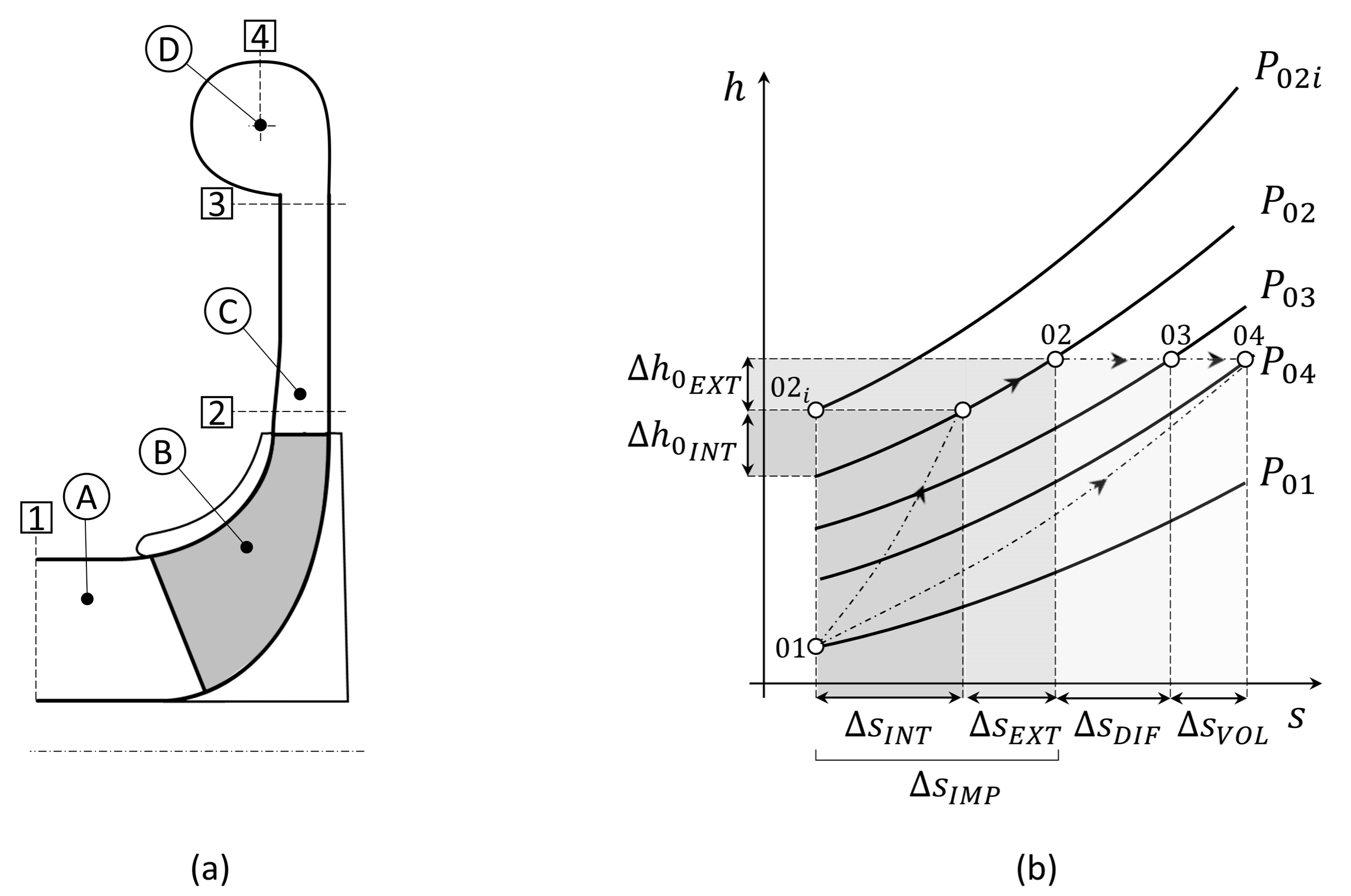
2.1. Step 1: 1D Single-Zone Model Implementation and Validation

Considering a single-stage centrifugal compressor composed of an impeller, a diffuser, and a volute (as shown in Figure 1a), a 1D single-zone model was developed based on Harley [51] and Amirante et al. [52]. In such a model, the flow properties were computed by solving energy and mass conservation, treating the operating fluid as a perfect gas. The impeller deviation angle was estimated using Qiu’s formulation [53], and the pressure drop across the inlet duct (Figure 1a, component A) was not taken into account, being negligible compared to the overall losses. Figure 1b depicts the thermodynamic compression through the stage and the effects on the enthalpy and entropy of the impeller, diffuser, and volute.
Concerning the impeller (Figure 1a, component B), internal and external losses were evaluated according to Oh [35] and Aungier [34]. Internal losses were divided into the incidence ( Δ h i n ), blade-loading ( Δ h b l d ), mixing ( Δ h m i x ), skin-friction ( Δ h s f ), choke ( Δ h c h ), and hub-to-shroud distortion ( Δ h h s ) losses. On the contrary, external losses were split into the recirculation ( Δ h r c ), disc-friction ( Δ h d f ), and leakage ( Δ h l k ) losses. Moreover, due to the main effect on impeller performance, incidence, blade-loading, mixing, and skin-friction losses were selected following Oh’s study [35]. Choke and hub-to-shroud distortion losses were added following Aungier’s study [34] to improve the accuracy near the choke condition. In the present work, clearance losses were not considered among the internal losses since the impeller was shrouded. However, these losses could be considered by adding the correlation proposed by Jansen [54]. As shown in Figure 1b, internal losses limited the total pressure ratio achievable by the impeller, while external ones caused an entropy increase with no effects on pressure.
Regarding the diffuser (Figure 1a, component C), in the present study, a vaneless configuration was investigated according to Amirante et al. [52]. Specifically, the methodology by Amirante et al. [52] and Stuart et al. [55] was used to investigate the pressure drop across the diffuser, while Staniz’s correlation [56] was leveraged to estimate the diffuser enthalpy loss. However, in case of a vaned diffuser, a similar approach can be applied, but using the enthalpy losses correlations indicated by Aungier [34]. Finally, concerning the volute (Figure 1a, component D), losses were divided into circumferential velocity, meridional velocity, skin-friction, and exit-cone losses according to Hazby et al. [57] and Weber and Koronowski [58]. For the sake of clarity, the loss correlations adopted for each component of the centrifugal compressor stage are summarized in Table 1. It is worth mentioning that these correlations have mainly been used with air as the working fluid. However, they have also been validated for other fluids, as reported by Ameli et al. [42] and Meroni et al. [59].
The developed 1D model was validated by comparing its predictions with CFD and experimental data of three different stages characterized by low, medium, and high flow rate, respectively. Comparisons were made in terms of total-to-total pressure ratio ( β t t ), polytropic efficiency ( η p ), work coefficient ( τ ), and polytropic head ( ψ ) defined as follows (Equations (1)–(4)).
β t t = p 02 p 01 ,
  η p = k 1 k ln p 02 p 01 ln T 02 T 01   ,
τ = c p T 02 T 01 U 2 2 ,
ψ = τ   η p = c p T 02 T 01 U 2 2 k 1 k ln p 02 p 01 ln T 02 T 01   ,
Moreover, the mass flow rate and the rotational speed of each machine were defined by means of the non-dimensional flow coefficient ( ϕ ) and peripheral Mach number ( M u ) as shown in Equations (5) and (6).
ϕ = 4 Q 01 π D 2 2 U 2 ,
M u = U 2 a 01 ,
The comparisons were conducted using measurements of the starting pre-engineered family available in the company. Such measurements included the geometric parameters of the family and their respective characteristic curves in terms of β t t ,   η p , τ , and ψ (Equations (1)–(4)), obtained at the impeller and diffuser outlet sections (Figure 1a, sections 2 and 3). For this reason, it was possible to validate the 1D model prediction of impeller and diffuser by comparing it to the results of CFD and empirical data. Conversely, the comparison between 1D model results and experimental measurements was not possible in the case of the volute (Figure 1a, section 4). Instead, another type of validation was performed by comparing 1D volute prediction with a simplified tool developed in-house by the company. Due to a non-disclosure agreement, the in-house tool and its results cannot be described; hence, the volute validation was not shown in the present work.
Concerning CFD analyses, RANS simulations were performed using the TRAF code [65], which is a 3D viscous solver based on the finite volume method for the resolution of Reynolds-Averaged Navier-Stokes equations on structured grids [66]. The discretization of convective fluxes was handled by a 2nd order TVD-MUSCL strategy build on the Roe’s upwind scheme, while a central difference scheme was used for the viscous fluxes. Wilcox’s k-ω model was employed for turbulence closure [67], and a high level of parallelization was ensured exploiting a hybrid OpenMP/MPI architecture [68]. The computational domain was discretized using H-type grids for the inlet duct, the rotor, and the diffuser (Figure 2). An overall grid of 3.5 million elements was selected after carrying out a sensitivity analysis, whose results are shown in Table 2. Indeed, increasing the number of elements beyond 3.5 million, the performance of the centrifugal compressor was no longer influenced by the adopted spatial discretization. Furthermore, to improve the predictive capability of the CFD analyses, the external losses shown in Table 1 were added to CFD results during the post-processing phase following the approach of Sundström et al. [40] and Harley et al. [69]. Table 3 summarizes the main assumptions of the numerical setup adopted for CFD analyses.
Experimental measurements were carried out with air at ambient conditions on a test rig available in the company. Pressure and temperature probes were positioned at the inlet and outlet sections of the impeller and diffuser, assessing their aerodynamic performance with an average error of less than 0.03%, 0.09%, and 0.79%, for temperature, pressure, and flow rate, respectively. As mentioned in Section 2.1, measurements were evaluated in the inlet section of the impeller, and in the outlet sections of both impeller and diffuser. Uncertainty propagation was then performed starting from the relative uncertainty of each sensor by means of in-house company -software. Systematic errors were assumed to be neglected since the pressure transducers are calibrated annually and the adopted thermocouples were provided with a calibration certificate.

2.2. Step 2: ANOVA

When looking for a suitable set of independent variables to adopt in a new family of centrifugal compressors, varying geometric parameters with negligible effects on performance could increase the time and the computational cost of the task without any benefit (also exacerbating the ANN training phase). On the contrary, adjusting only significant parameters could reduce the design efforts. In this perspective, four activities were carried out to highlight the significant independent parameters, while excluding from the study the non-significant ones. As a first activity, all the independent input variables used as design variables were identified based on Shouyi et al. [70] and on the company’s know-how. However, it is worth mentioning that, as suggested by Aungier [34], unlike Shouyi et al. [70], the impeller axial length was not considered as an independent variable, but computed following the equation in ref. [34]. The resulting independent variables are shown in the first column of Table 4. In the second activity, a range of three realistic values was associated to each independent variable. Specifically, the two range extremes (upper and lower bounds) were selected based on experts’ know-how in terms of expected aerodynamics effects and manufacturability issues. The third (intermediate) value was then calculated as arithmetic mean of the upper and lower extremes. In addition, a further comparison was made with the ranges provided by Shouyi et al. [70]. The second column of Table 4 shows the specific ranges considered in the present study to achieve the desired EC family. It is worth noting that, since our aim was to achieve a new family of centrifugal compressors with inlet hub diameter and outlet diameter, no range of variation was considered for such independent variables. Instead, constant values were imposed as reported in Table 4. Subsequently, in the third activity, combining the variable values of Table 4, a total of 6561 perturbed geometries were generated and submitted to the 1D model at stall, design, and choke conditions (where the design condition was the point with peak efficiency, the stall condition the point with horizontal tangent of the polytropic head, and the choke condition the point at which the stage polytropic efficiency was reduced by 10%). This was carried out for three different stages characterized by low, medium, and high flow rates. Finally, in the fourth activity, the results of the 1D model predictions were subjected to an ANOVA to assess the impact of each independent variable of Table 4 on the stage performance [71]. The ANOVA (with main effect plot) was performed with the Minitab software, allowing variables to assume three discrete values to obtain easily understandable graphs in which the impact could be immediately recognized. Based on the ANOVA results, the non-significant independent variables were excluded from the study (associating them with constant values), while considering in the next steps the remaining significant independent variables.

2.3. Step 3: Sobol Sequence

Having removed non-significant parameters, a new dataset was generated to feed and train an ANN as follows. A sample of feasible geometries was generated by associating realistic values with the remaining independent variables. To this aim, unlike the ANOVA (step 2), here variables were assigned by means of a Sobol quasi-random low discrepancy sequence [72], rather than adopting only three discrete values. In this perspective, the value of each independent variable was varied based on Equation (7), where J is the total number of realistic compressor geometries to be created, j is the specific geometry considered, I is the total number of remaining independent variables emerged in step 2, i is the specific independent variable to which we are assigning a value x i j , x l i and x u i are the variable upper and lower limits, and S i j depends on the Sobol sequence.
x i j = x l i + S i j · x u i x l i                     w i t h   i = 1 , , I   a n d   j = 1 , , J ,
Then, 2500 possible realistic geometries were achieved by combining the values of the independent variables. Next, each of these geometries was analyzed with the 1D model to predict total-to-total pressure ratio, polytropic efficiency, work coefficient, and polytropic head (Equations (1)–(4)) at section 4 (Figure 1a) for stall, design, and choke conditions. Subsequently, a dataset composed by the values of the significant independent variables and the respective performance predictions was collected and used to train and validate an ANN. The Sobol sequence was adopted to link variables with quasi-random values based on Burhenne et al. [73]. Indeed, as stated by the authors themselves, when a large number of independent input variables are affecting a problem, the Sobol sequence is more effective than other sequences such as Latin Hypercube or Monte Carlo sampling.

2.4. Step 4: Artificial Neural Network

The obtained Sobol-based dataset emerged in step 3 was used to train and validate an ANN, thus obtaining a response surface capable to reproduce the 1D model behavior. Specifically, a feed-forward ANN with two hidden layers was adopted and trained by means of a back propagation algorithm. By using 70% of the obtained Sobol-based dataset (the remaining 30% was used in equal parts for testing and validation), the training process was carried out in accordance with Riccetti et al. [74], aiming to minimize the difference between the ANN prediction and the 1D model results. To better understand this process, let us consider an input vector (from now on called x ) composed of the independent variables achieved in step 2, and an output vector (here referred to as y ) composed of the stage performance calculated through the 1D model (Equations (1)–(4)). Considering the 1D model as a function f , the y vector is obtained starting from x as follows (Equation (8)).
y = f x ,
Starting from the same x , the ANN prediction (here referred to as y ) can be defined based on Equation (9), where g represents the behavior that the ANN learned to forecast during the training process.
y = g x ,
The ANN response surface g being a surrogate model of the 1D model f , it might be possible that the ANN prediction y differs from the 1D model output y . For this reason, the training process was conducted by minimizing the prediction error ϵ defined as follows. Specifically, ϵ was minimized by recursively performing the training process and updating, for several times (epochs), the weights used to manage the passage of information through neurons.
ϵ = y y 2 ,
Once the ANN was trained, a k-fold cross-validation process was performed to understand the ANN reliability and avoid under-fitting and over-fitting issues. This activity completed the ANN construction phase.
Then, exploiting a random search algorithm [75], a new sample of possible geometries was built and given as input to the ANN. Therefore, from the ANN predictions, a Pareto front was found.

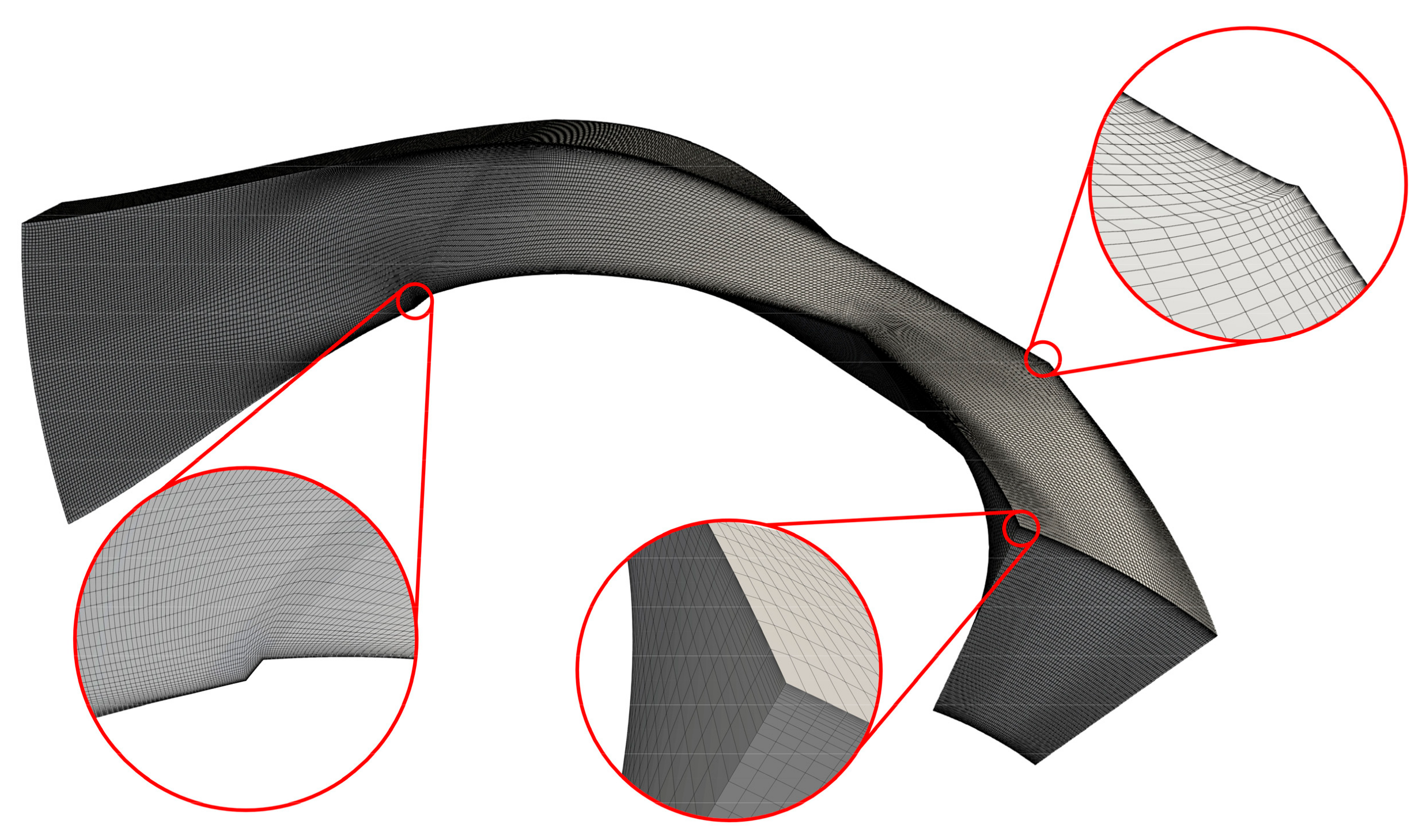
2.5. Step 5: Validation of Promising Solutions through CFD Analyses

Finally, a further validation of the obtained results was carried out as follows. Some promising solutions of the Pareto front were selected, each of the selected solutions was analyzed with CFD simulations, and the obtained results were compared with the ANN predictions (analyzing the values of total-to-total pressure ratio, polytropic efficiency, work coefficient, and polytropic head). Finally, once we validated the results of the ANN, one of the promising solutions was chosen and designated as a stage of the new centrifugal compressor family.

3. Results and Discussion

The methodology proposed in Section 2 was applied, as an example case study, to derive a new family of EC impellers from an existing family of LNG centrifugal compressors. For the sake of clarity, instead of showing the results obtained for each impeller of the family, the results are shown for three different stages characterized by low, medium, and high flow, respectively. Indeed, these stages are well representative for the whole family and the obtained considerations could be easily extended to intermediate stages. The following subsections describe and discuss the achieved results following the subdivision provided in Section 2.

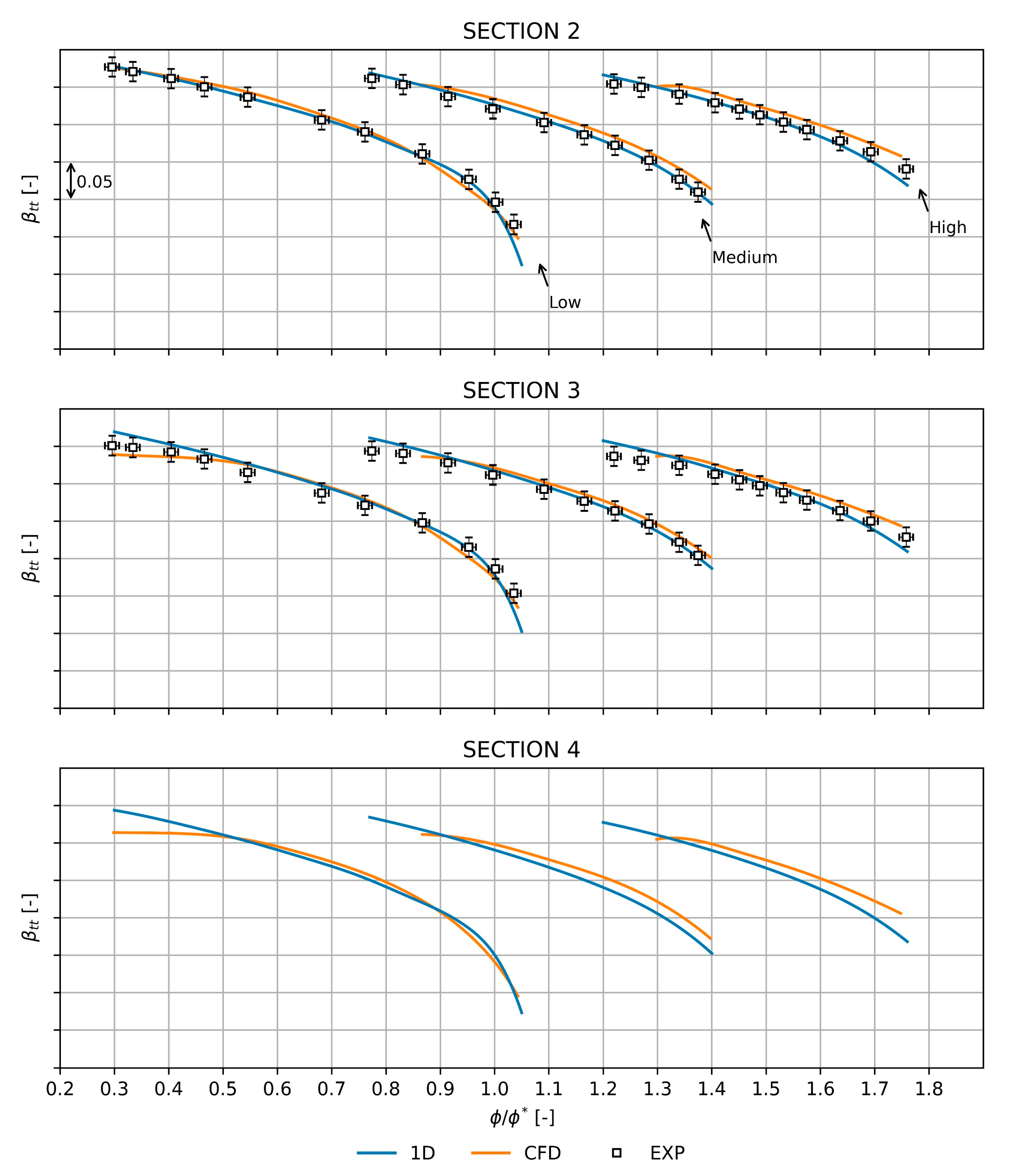
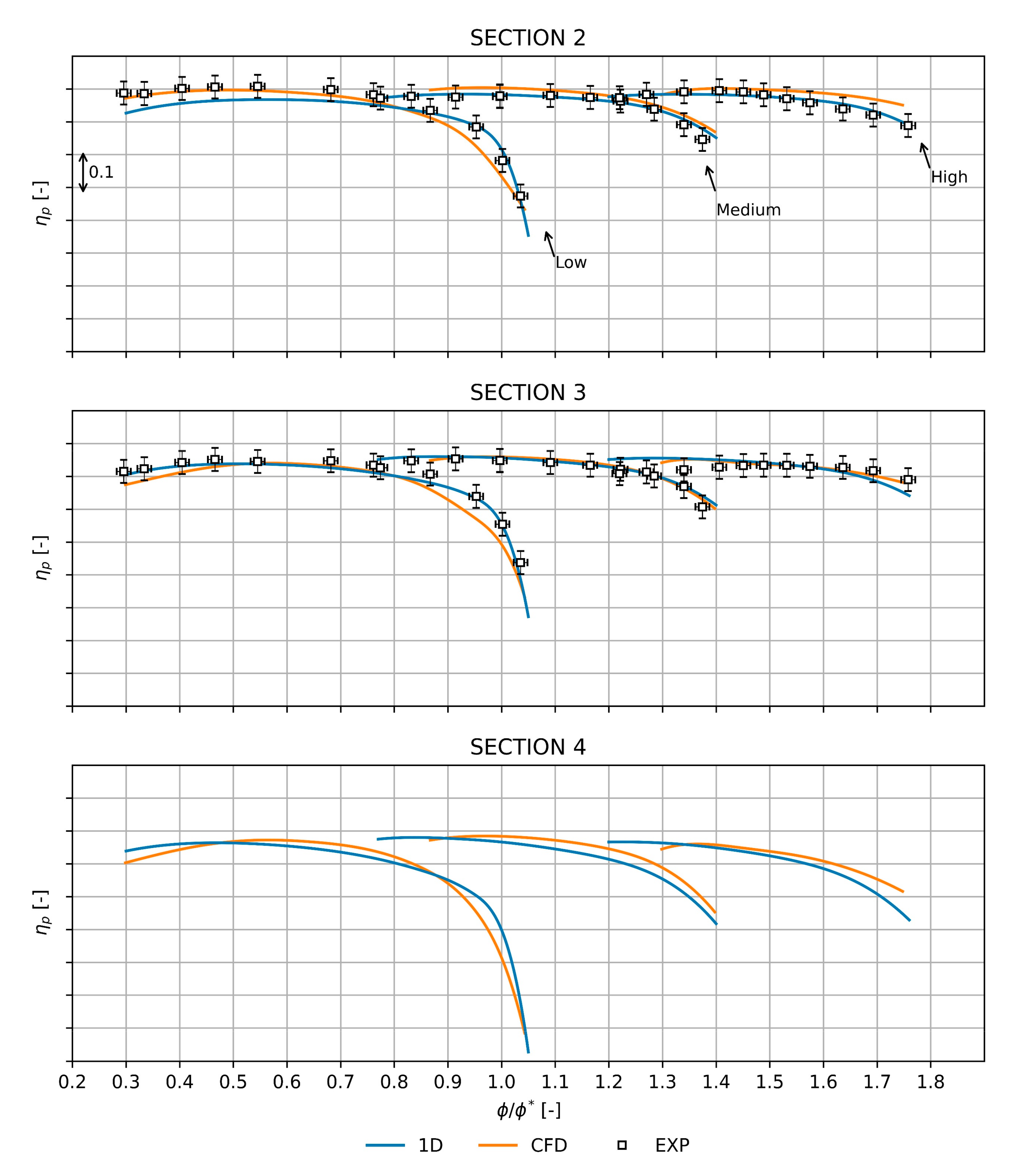
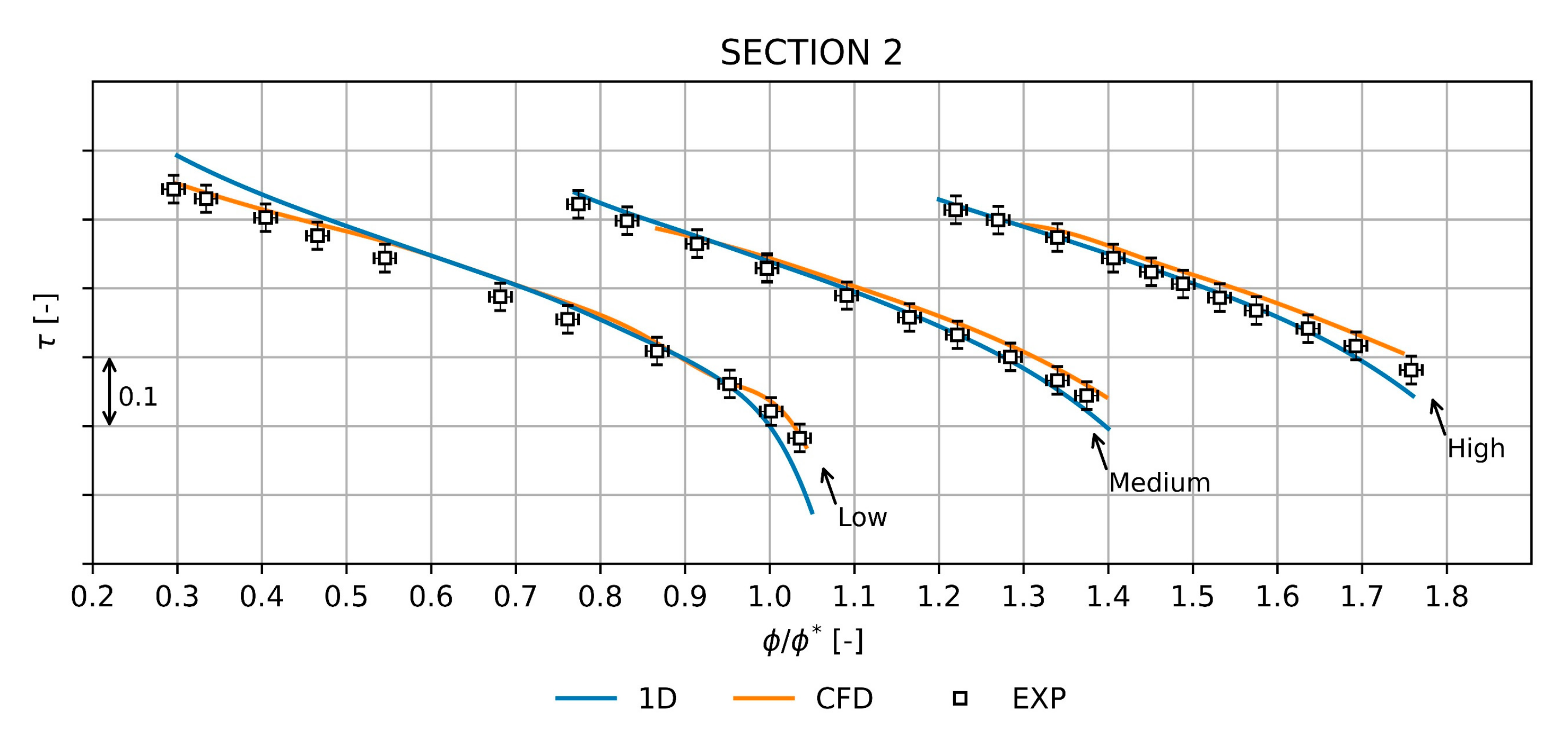
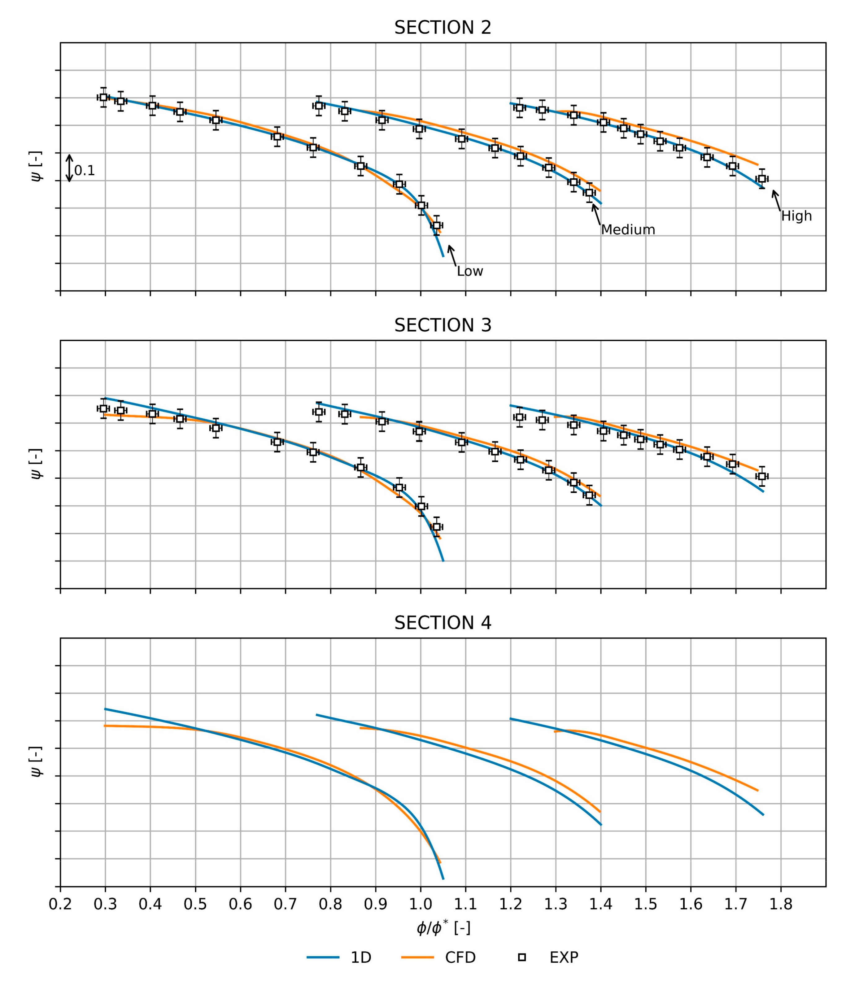
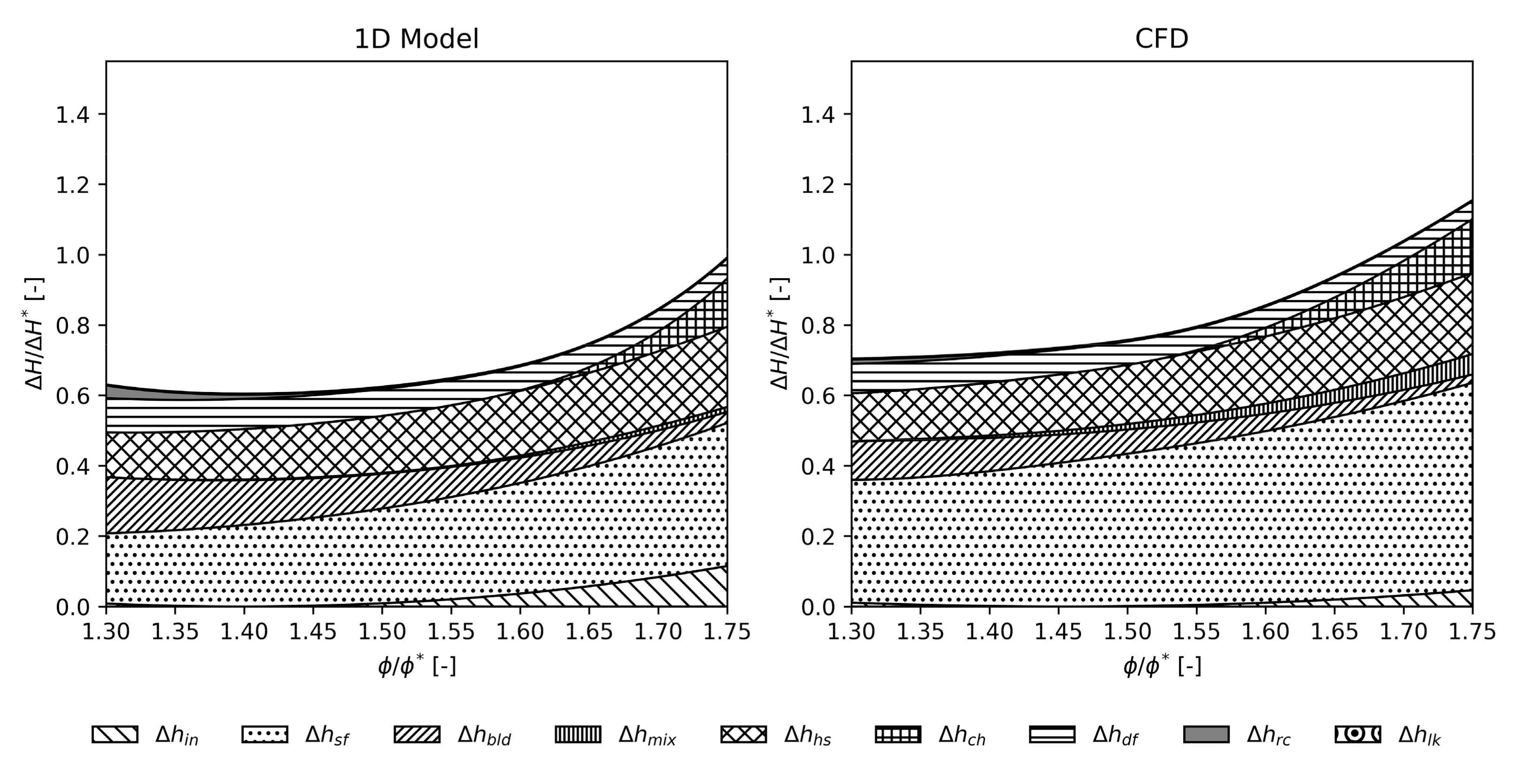
3.1. Step 1: Validation of 1D Single-Zone Model

The implemented 1D single-zone model was validated by comparing its predictions with CFD and experimental data in terms of β t t ,   η p , τ , and ψ (Equations (1)–(4)) at sections 2 and 3 of Figure 1a. While in section 4 (volute outlet), due to the absence of available experimental data, the validation was performed by comparing the 1D volute prediction with the company CFD-based in-house tool. It is worth mentioning that for this case study a vaneless diffuser was adopted, but the developed 1D model could also be applied with vaned configurations. Figure 3 shows the β t t trend for the three stages designed for low (left-hand curves), medium (middle curves), and high flow rate (right-hand curves), respectively. At impeller outlet (section 2), a good agreement between the 1D model (blue lines) and the experimental data (white squares) was observed for each machine. The CFD analyses (orange lines) instead showed a slight over-estimation of the total-to-total pressure ratio. A similar behavior was recorded at the diffuser outlet (section 3). The 1D model seemed to follow the trend of the experimental data, except near the stall where the slope variation of the curve was not correctly replicated. However, in the worst case (low flow stage, left-hand curves) the percentage deviation was less than 1.94%. Moreover, it can be observed that the 1D model allowed reaching the stall condition, while the performed RANS simulations were not able to analyze it, especially in the medium and high flow stages. Focusing on the volute output (section 4), the 1D model showed an underestimation of β t t compared with the CFD-based in-house tool. This discrepancy is more relevant when increasing the flow coefficient at which the stage is designed.
In Figure 4, the comparison between the 1D model, the CFD, and the experimental data is conducted in terms of η p . In this case, a good agreement was reached at the diffuser outlet (section 3), while the same discrepancies were present at sections 2 and 4. Specifically, the worst percentage deviation of the 1D model was about 4.98% in comparison with experimental data at section 2, and near 3.55% compared with the CFD-based in-house tool at section 4. However, such differences can be considered acceptable, since the 1D model intrinsically simplifies the highly three-dimensional flow field of the centrifugal compressor.
Regarding the work coefficient τ (Figure 5), the medium and high flow coefficient stages showed a 1D prediction close to the CFD and experimental data. Indeed, the average percentage error in these cases was about 1.15%, while for the low flow stage it rose to 2.88%. In Figure 5 only section 2 is shown, since the diffuser and volute, being static components, do not increase the total enthalpy rise of the stage.
The comparison shown in Figure 6 highlights how the 1D model can replicate the experimental data in terms of ψ . Compared with the CFD results, the 1D predictions appear closer to the experimental measurements, as evidenced by an average percentage error of 2.10% instead of 3.25% for the CFD analysis. This trend remained unaltered at the exit of the volute (section 4).
Figure 7, Figure 8 and Figure 9 show the comparison between the 1D model and CFD analyses related to the impeller loss sources for the three stages. As it can be noticed, the loss trends resulting from the 1D model were consistent with those computed with the CFD simulations. Although the skin friction losses ( Δ h s f ) were underestimated in the 1D model, the overestimation of the incidence losses ( Δ h i n ) appeared to compensate for this underestimation, providing a correct overall assessment. On the other hand, the other sources of losses were comparable between the 1D and CFD models in terms of values and shapes. Furthermore, from Figure 7, Figure 8 and Figure 9 it is possible to appreciate the relative impact of each loss source, in accordance with the Oh’s findings [35]. As a unique difference with Oh’s study, the 3D geometry of the realized impellers made the adoption of choke and hub-to-shroud distortion losses proposed by Aungier [34] unavoidable.

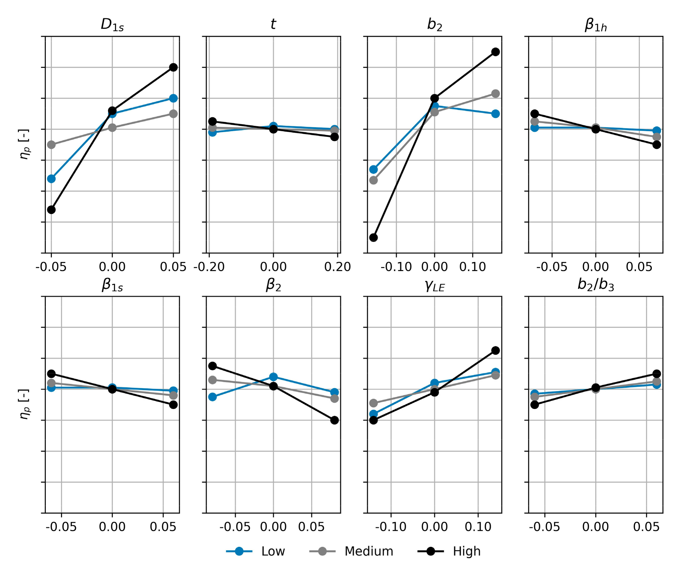
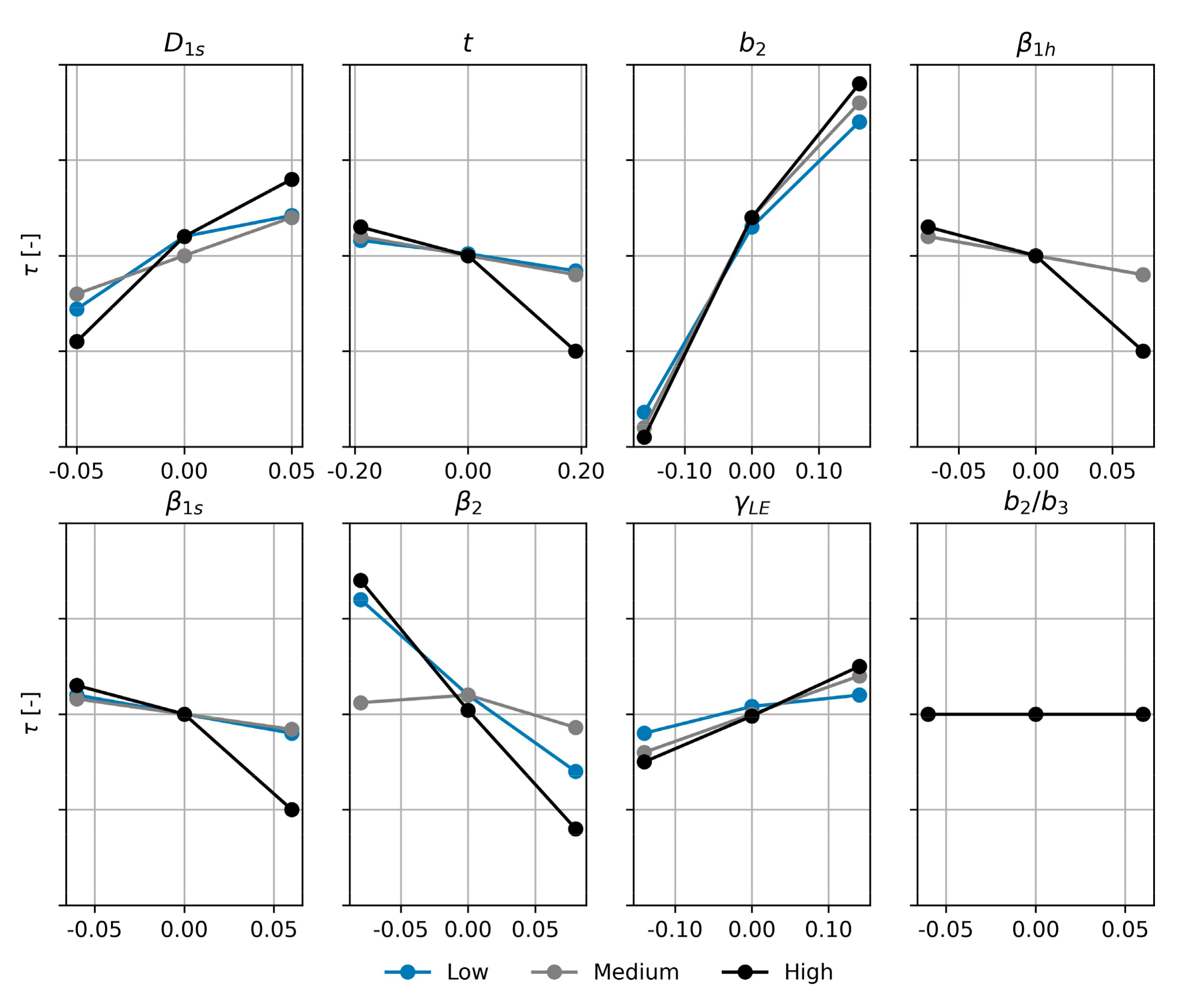
3.2. Step 2: ANOVA Results

The ANOVA was performed to assess the impact on stage performance of each independent variable of Table 4, thus excluding non-significant ones from the study. To conduct the ANOVA, the values of the independent variables were varied by creating a set of 6561 possible geometries, where D 1 h , D 2 , and the number of blades were fixed to meet the new family requirements. Figure 10 and Figure 11 depict the ANOVA outcomes (in terms of main effect plot) related to η p   and τ , for the low (blue), the medium (gray), and the high flow coefficient stage (black), respectively. Similar results were achieved for β t t   and ψ but were not reported here for the sake of brevity. Figure 10 and Figure 11 prove that none of the independent variables of Table 4 had a negligible impact on the stage performance. Hence, all independent variables were considered in the next steps of the present study to feed and train the ANNs and derive the new centrifugal compressor family.

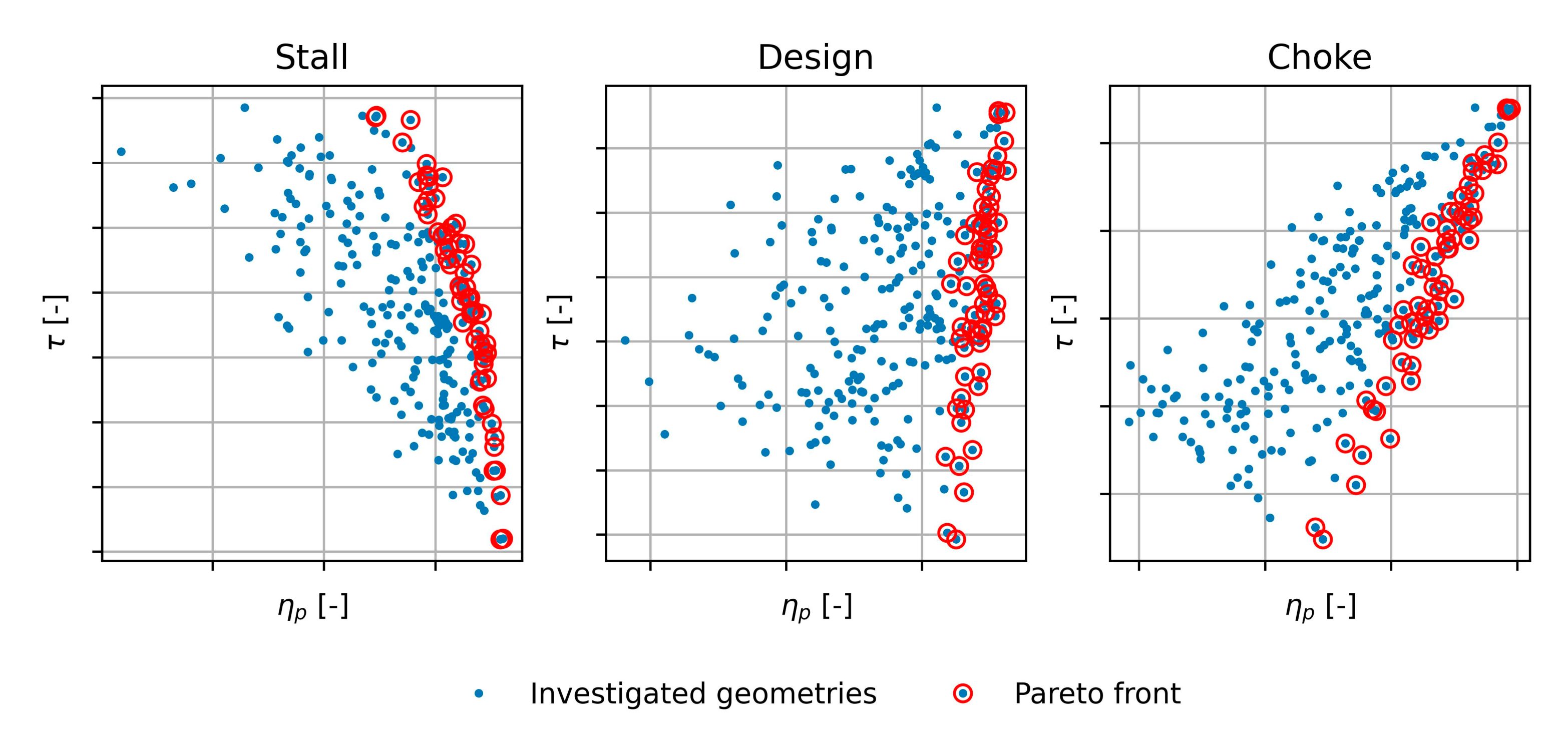
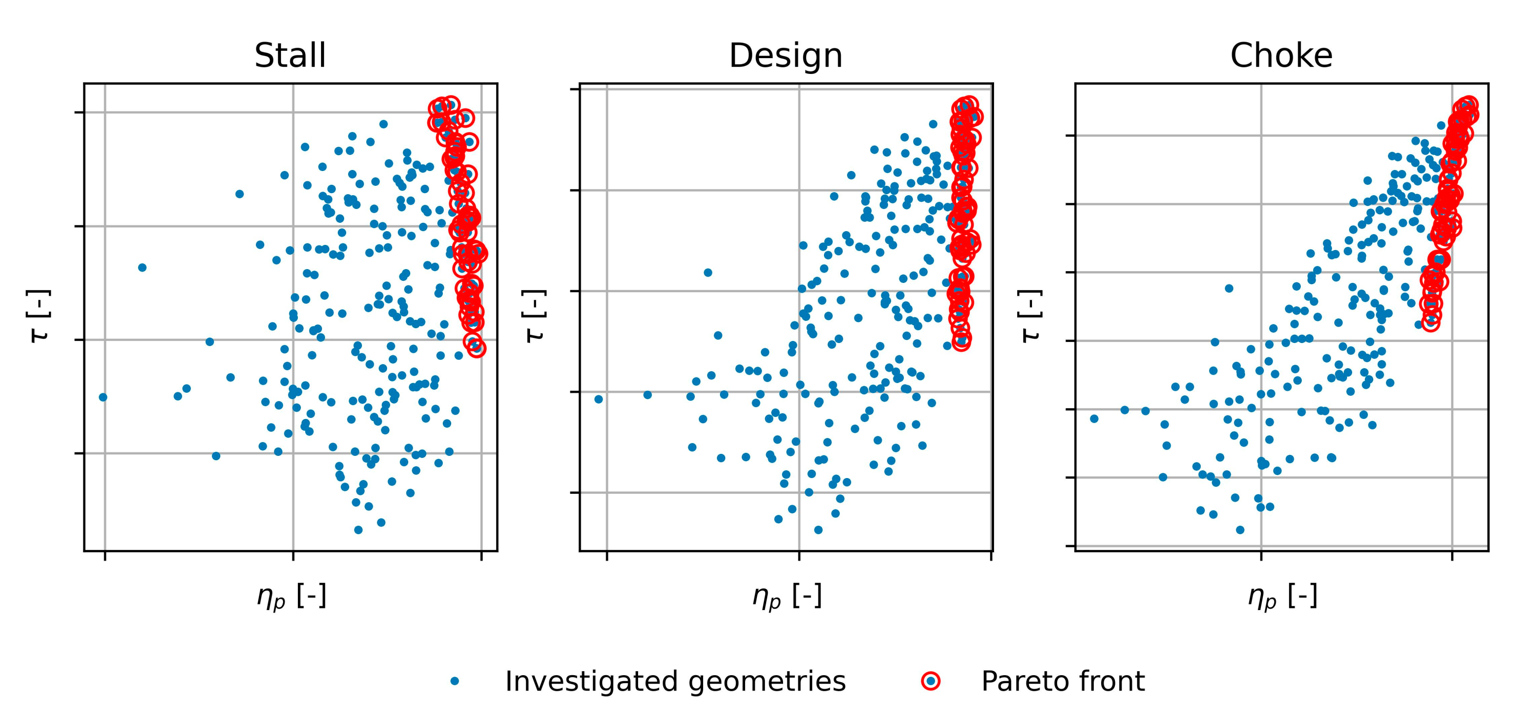
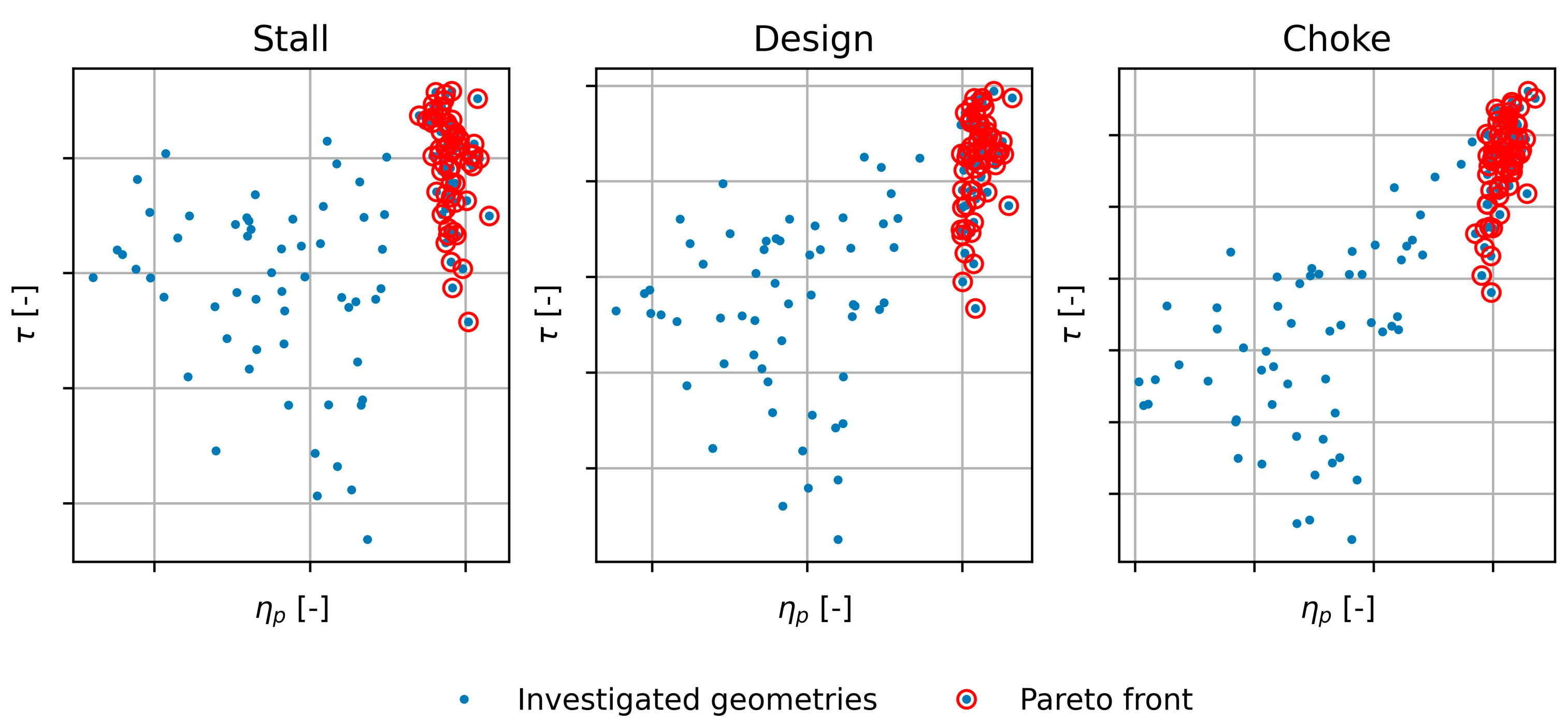
3.3. Step 3: Sobol Sequence

Exploiting a Sobol sequence (Equation (7)), a range of realistic values was associated with each non-negligible independent parameter emerging from step 2 (Section 2.2 and Section 3.2). As a result, a dataset of 2500 possible geometries was achieved for each stage of the family. Then, the 1D model was applied to each geometry belonging to the dataset, thus predicting the stage performance, and conducting three parametric analyses (one for each analyzed stage).

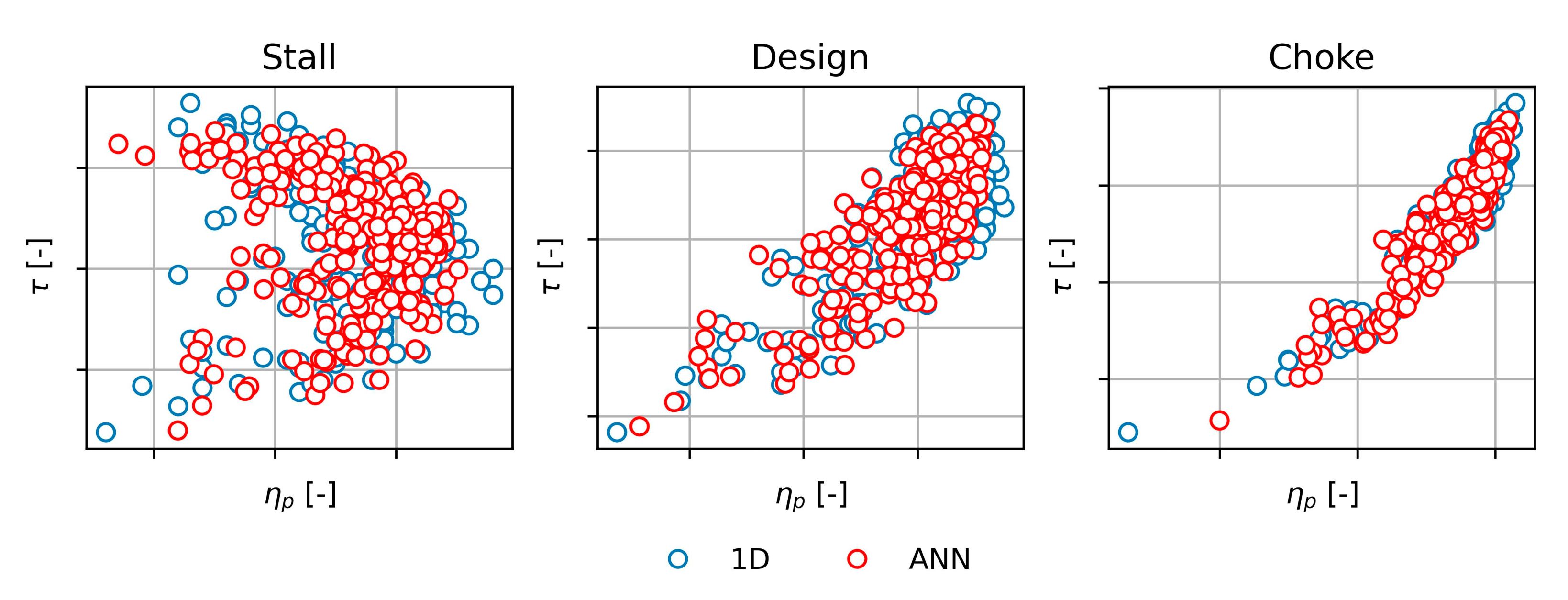
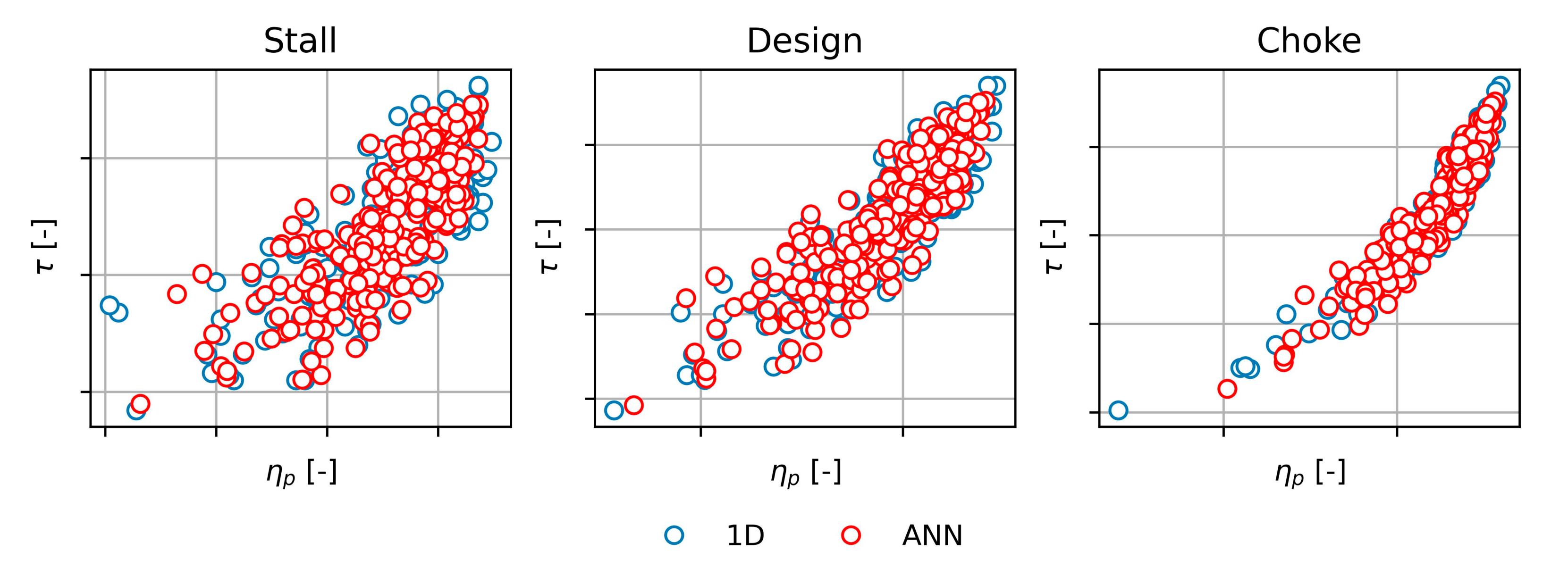
3.4. Step 4: Artificial Neural Network

The results of each parametric analysis were used to feed and train a related ANN. Consequently, three ANNs were obtained, one for each stage of the family. Figure 12, Figure 13 and Figure 14 show the results of the ANN training process, comparing the 1D model prediction (blue dots) associated to each test geometry and the respective ANN forecast (red dots), in terms of η p   and τ . Like in step 3, similar results were achieved for β t t   and ψ but were not reported for the sake of brevity. ANNs showed a good predictive capacity, as evidenced by the forecast absolute errors ( ϵ η p and ϵ τ ) presented in Table 5 and calculated as the average of differences between each ANN forecast and its related 1D model prediction (expressed as a percentage). It is worth mentioning that the time required on a personal computer (Intel Core i7, 8 cores at 4.80 GHz and 32 GB DDR4 memory at 3200 MHz) to produce the database for the ANN training and the subsequent training phase was less than 6 h. This time was mainly due to the recursive use of the 1D model, which accounted for about 70% of the total time. However, once the ANN was trained, the resulting meta-model predicted the performance of one stage in less than 0.2 s, while the 1D model took two orders of magnitude longer. By using the proposed approach, the initial design time of the three stages was reduced by 75% compared with the procedure currently used in the company. Moreover, if the dataset is large enough, the same ANN could be used to design more than a single stage, further reducing design time.
ϵ η p ϵ τ ϵ η p ϵ τ ϵ η p ϵ τ Once the ANNs were trained and validated, such meta-models were used in conjunction with a random search algorithm [75] to predict, for each of the three stages, the performance of a new sample of possible geometries. Based on the achieved predictions, three Pareto fronts were built, one for each stage.
Figure 15, Figure 16 and Figure 17 depict all the investigated geometries (blue dots), also highlighting the optimal solutions composing the Pareto front (red circles).

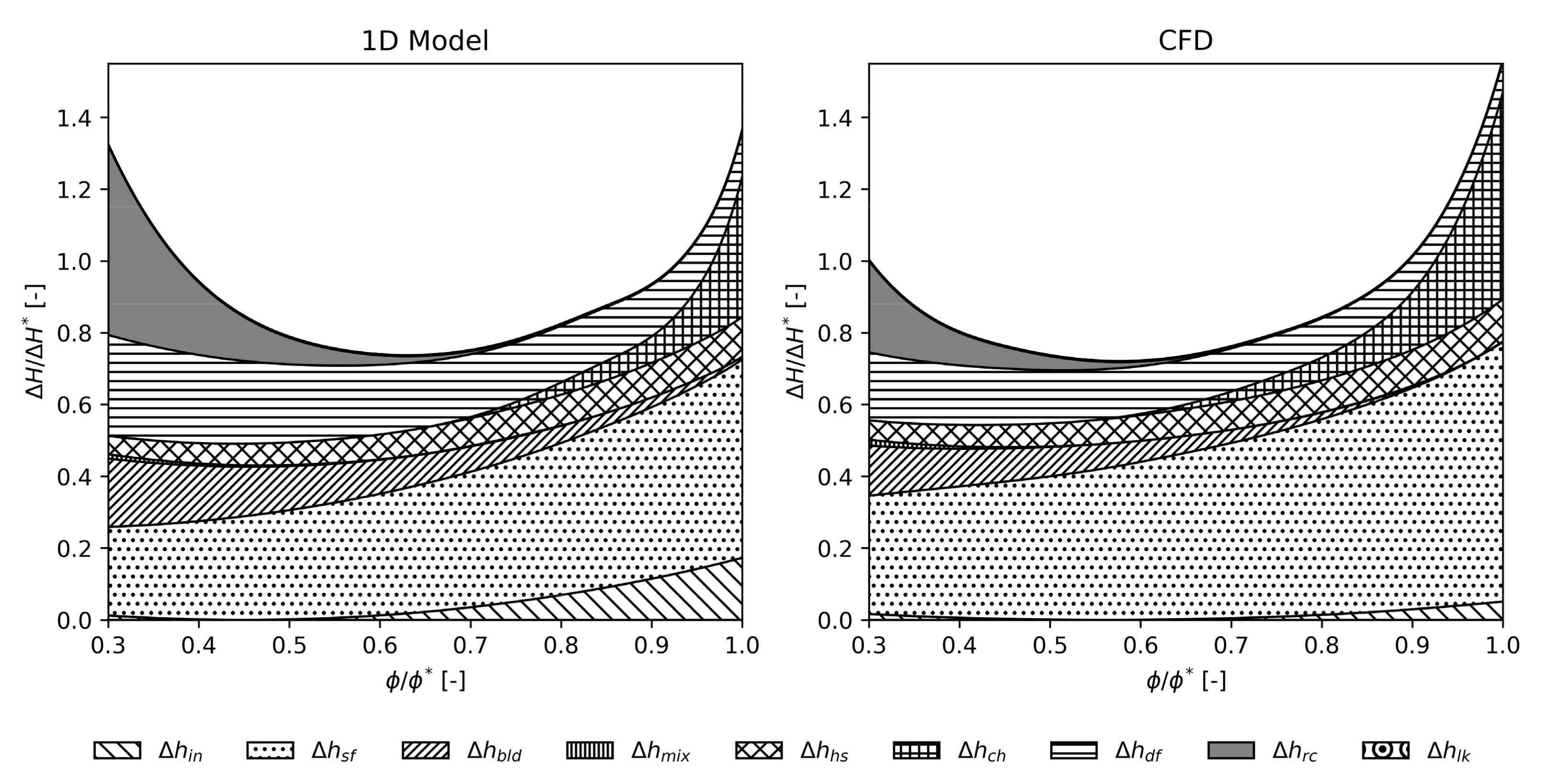
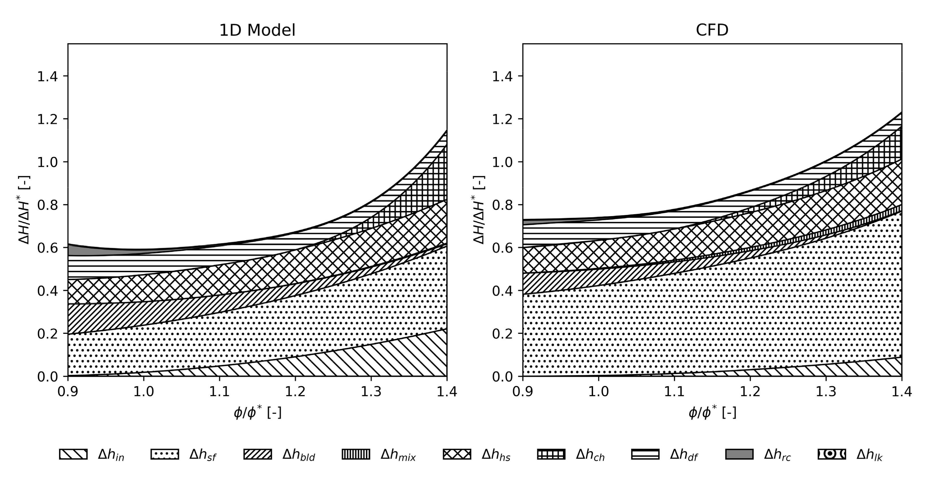
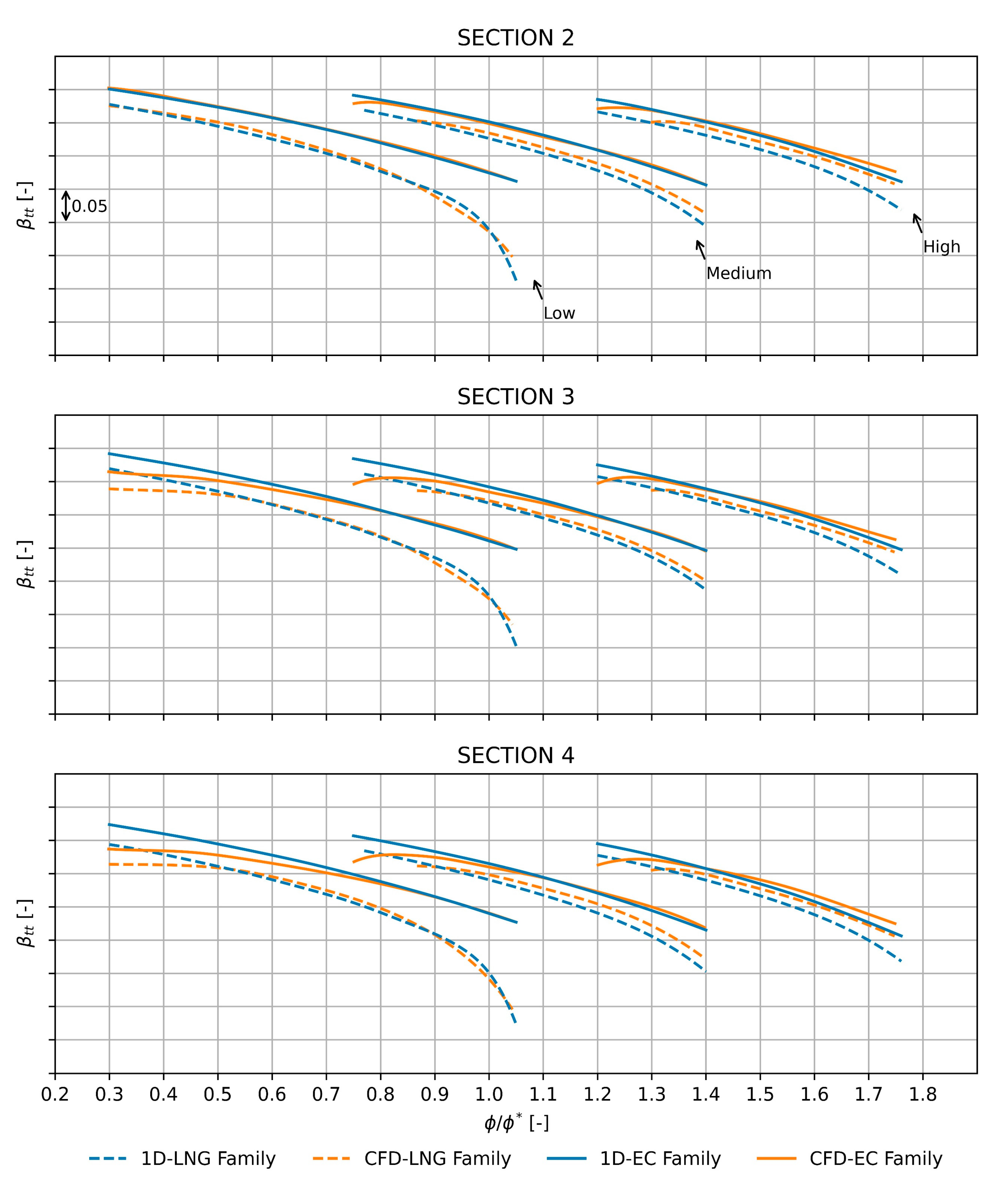
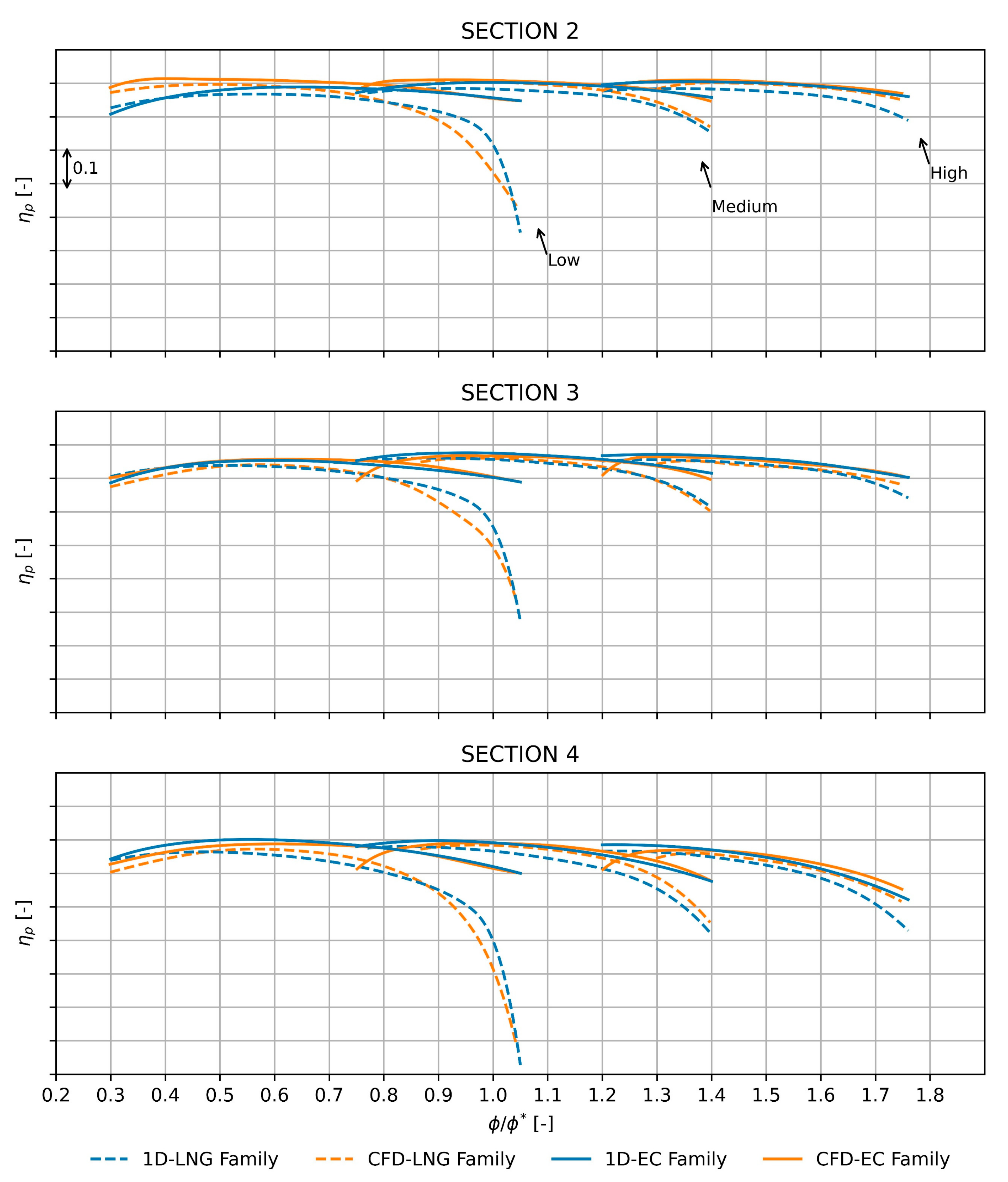
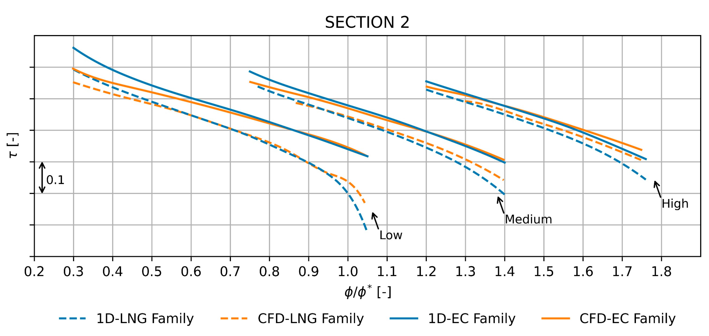
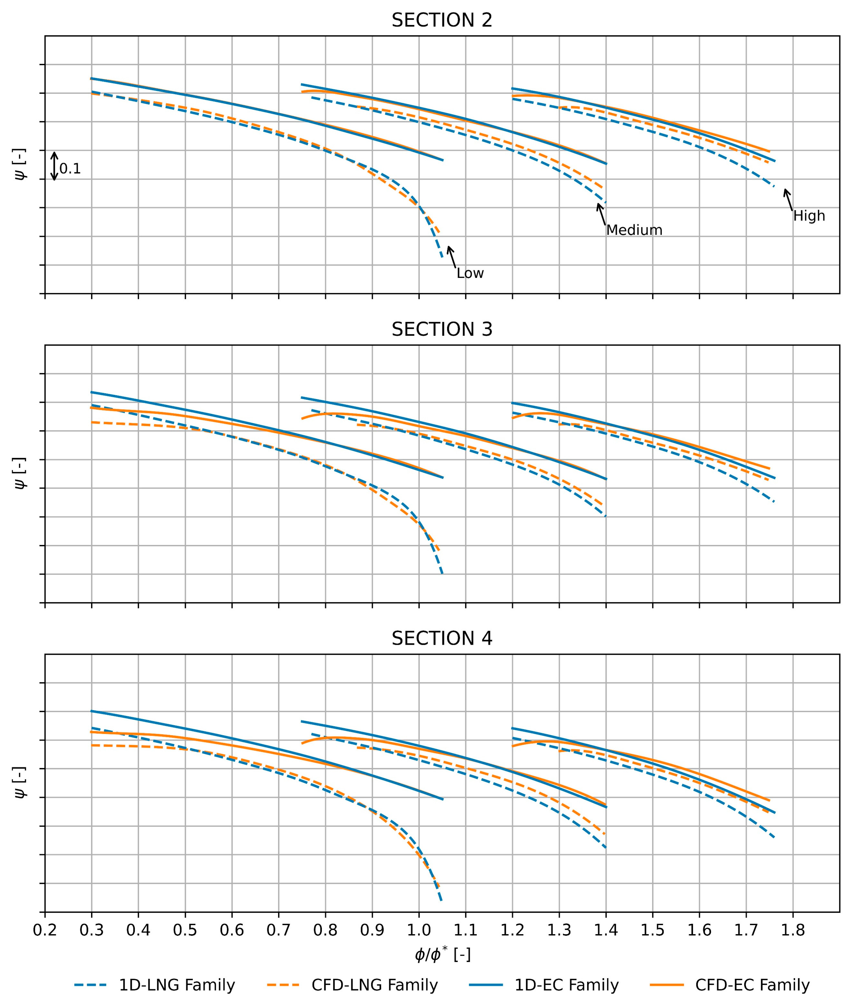
3.5. Step 5: Validation of Promising Solutions through CFD Analyses

Among the optimal geometries of each Pareto front, five were selected as being the most promising (for a total of fifteen geometries). These machines were, then, validated through CFD analyses. Finally, the three geometries considered by company experts to represent the optimal trade-off between performance and geometric characteristics (e.g., size, manufacturability, mechanical strength, and so on) were selected. These geometries laid the foundation of the new family of centrifugal compressors for EC applications. Figure 18, Figure 19, Figure 20 and Figure 21 show the comparison between the stage performance of the existing LNG family and the ones of the derived EC family in terms of β t t ,   η p , τ , and ψ . Each derived machine provides better performance than the original family. In addition, the stall and choke margins were extended, thus increasing the operating range of each machine. Finally, the comparisons showed, once again, a good agreement between the 1D model and CFD.

4. Conclusions

The current efforts related to energy transition, the reduction of greenhouse gas emissions, and other sustainability issues are expected to induce, in the future, lumpy and unpredictable changes in the demand of centrifugal compressors. For this reason, a valuable way to quickly react to demand fluctuations is highly claimed by compressor manufacturers. In this context, the combined use of a 1D single-zone model and ANNs has been identified as a sound way to exploit the know-how of existing impeller families, highlight relationships between geometrical parameters and performance of existing machines, and shorten and streamlining the new product aerodynamic design process by modifying the characteristics of existing compressors to generate new optimized machines. However, the literature lacks studies on the joint use of a 1D single-zone model with an ANN for designing new centrifugal compressor families starting from pre-engineered ones.
To fill this gap, the present paper proposed a new model (testing it on the case study of a new expander-compressor impeller family derived from existing natural gas liquefaction machines), which involved performing five main steps: (i) a 1D single-zone model was built to predict the performance of the impeller, diffuser, and volute of centrifugal compressors, which was validated through a comparison with experimental data and CFD analyses; (ii) the most relevant independent input variables required to apply the 1D model were identified (leading to eight independent variables). Then, an ANOVA was conducted, proving that all these variables had a consistent (non-negligible) impact on the results of the 1D model predictions; (iii) an extensive parametric analysis was performed for each compressor stage analyzed, investigating three main compressor stages (designed for low, medium, and high flow rate). Then, assigning Sobol quasi-random values to the relevant independent input variables, a total of 2500 geometries were defined for each compressor stage. Next, each geometry was submitted to the 1D single-zone model, defining for each geometry its performance in terms of total-to-total pressure ratio, polytropic efficiency, work coefficient, and polytropic head; (iv) the results of the parametric analyses were used to feed and train an ANN for each compressor stage analyzed. Then, the ANNs forecasts were used to build a Pareto front for each compressor stage analyzed, thus identifying fifteen promising compressor solutions, in agreement with company experts; (v) finally, the performance of these fifteen solutions forecasted by the ANN were validated through a comparison with CFD analyses, also identifying the three geometries (one per each compressor stage analyzed) that represented the optimal trade-off between aerodynamic performance and geometric characteristics.
The results of the present paper showed that the proposed model enables developing a new family of centrifugal compressors starting from an existing one, improving the initial performance while containing design time and computational efforts in favor of further 3D optimizations. Moreover, results proved that the combined use of a 1D single-zone model and an ANN leads to reliable predictions, determining low absolute errors (always below 1.0%) in the forecast of compressor performance (compared to only 1D prediction). Finally, the results of this study showed that exploiting the know-how of existing machines to design new compressor families significantly shortened the new product aerodynamic design process. In fact, applying the new model to the case study here proposed allowed the design of three different compressor stages in less than one week (against one month usually required by the staff of the company investigated to obtain similar results).
Overall, the main contribution of this study is represented by the five-step model based on the combined use of a 1D single-zone model and an ANN. Indeed, to the best of the authors’ knowledge, nothing similar has been provided by the literature so far to design new centrifugal compressor families starting from pre-engineered ones, thus shortening the new product aerodynamic design process.
It is worth mentioning that the proposed model can be applied to any kind of centrifugal compressor, although the present study showed an application to the specific case of overhang centrifugal compressors for EC application. However, it is worth noting that the results of the proposed model are based on the following simplifying assumptions: the flow through the compressor stage is one-dimensional, the flow properties are assumed uniform at each stage section, and the loss correlations are assumed to correctly predict the real losses through the compressor stage.
Future developments of this research could be twofold. First, to study the impact that technical specifications (e.g., the skin friction coefficient or the factor for incidence loss), imposed as design input choices, have on the model predictions, especially focusing on the influence of these factors on the 1D single-zone model forecasts. More in detail, we could define if the new proposed model is robust, or it changes its performance accuracy when varying the imposed input parameters. Secondly, to include in the new proposed model the analysis of manufacturing non-conformities, studying from the company databases the non-conformities that occur more frequently, then exploiting artificial intelligence to obtain, among all the possible compressor geometries, the ones whose performance are more robust and reliable against manufacturing uncertainties and variability in geometrical properties.
Authors should discuss the results and how they can be interpreted from the perspective of previous studies and of the working hypotheses. The findings and their implications should be discussed in the broadest context possible. Future research directions may also be highlighted.

Author Contributions

Conceptualization, M.B., D.B. and M.M.; methodology, M.B.; software, M.B.; validation, M.B., M.M. and D.B.; formal analysis, M.B.; investigation, M.B. and D.B.; resources, F.C. and A.A.; data curation, M.B., L.T. and M.M.; writing—original draft preparation, M.B.; writing—review and editing, M.B., D.B., M.M., L.T. and F.C.; visualization, M.M. and L.T.; supervision, M.M., D.B., A.A. and F.C.; project administration, A.A. and F.C.; funding acquisition, A.A. and F.C. All authors have read and agreed to the published version of the manuscript.

Funding

This research received no external funding.

Institutional Review Board Statement

Not applicable.

Data Availability Statement

Not applicable.

Acknowledgments

The authors thankfully acknowledge Baker Hughes and the centrifugal compressor aerodynamic team of Nuovo Pignone-Baker Hughes for the technical support received during the project.

Conflicts of Interest

The authors declare no conflict of interest.

Nomenclature

A Area
a Velocity of sound
b Blade height
c Absolute velocity
c f Friction coefficient
C p Specific heat ratio
D Diameter
D f Diffusion factor
f i n c Incidence factor
H Entalpy
h Specific entalpy
k Specific heat ratio
L Blade length
m ˙ Mass flow rate
M u Peripheral Mach number
P Pressure
Q Volume flow rate
r Radius
s Specific entropy
T Temperature
t Thickness
U Peripheral velocity
w Relative velocity
Z Effective number of blades
Δ Variation
α Absolute angle
β Relative angle/pressure ratio
γ Blade slope angle
ε Wake fraction of blade-to-blade space
η Polytropic efficiency
τ Work coefficient
ϕ Flow coefficient
ψ Polytropic head
Subscripts
0Total quantity
1Impeller inlet
2Impeller outlet
3Diffuser outlet
4Volute outlet
blBlade
bldBlade loading
chChoke
clClearance
dfDisc friction
eExit cone
hhub
hsHub-to-shroud distortion
hydHydraulic
inincidence
LELeading edge
lkleakage
mMeridional component
mixmixing
pPolytropic
rcRecirculation
sShroud
sfSkin friction
splSplitter
TETrailing edg
thThroat
ttTotal to total
uCircumferential component
vcvVolute circumferential velocity
vldVaneless diffuser
vmvVolute meridional velocity
vsfVolute skin friction
Superscripts
*Sonic condition/scaling factor
-Average

References

  1. National Oceanic and Atmospheric Administration. Available online: http://www.noaa.gov/ (accessed on 28 October 2021).
  2. Climate Change: Vital Signs of the Planet. Available online: https://climate.nasa.gov/ (accessed on 28 October 2021).
  3. Climatic Research Unit-Groups and Centres-UEA. Available online: https://www.uea.ac.uk/groups-and-centres/climatic-research-unit (accessed on 28 October 2021).
  4. IPCC. Climate Change Widespread, Rapid, and Intensifying, IPCC. Available online: https://www.ipcc.ch/2021/08/09/ar6-wg1-20210809-pr/ (accessed on 28 October 2021).
  5. UNFCCC. The Paris Agreement. Available online: https://unfccc.int/process-and-meetings/the-paris-agreement/the-paris-agreement (accessed on 21 September 2021).
  6. Rockström, J.; Gaffney, O.; Rogelj, J.; Meinshausen, M.; Nakicenovic, N.; Schellnhuber, H.J. A Roadmap for Rapid Decarbonization. Science 2017, 355, 1269–1271. [Google Scholar] [CrossRef]
  7. De La Peña, L.; Guo, R.; Cao, X.; Ni, X.; Zhang, W. Accelerating the Energy Transition to Achieve Carbon Neutrality. Resour. Conserv. Recycl. 2022, 177, 105957. [Google Scholar] [CrossRef]
  8. Ram, M.; Osorio-Aravena, J.C.; Aghahosseini, A.; Bogdanov, D.; Breyer, C. Job Creation during a Climate Compliant Global Energy Transition across the Power, Heat, Transport, and Desalination Sectors by 2050. Energy 2022, 238, 121690. [Google Scholar] [CrossRef]
  9. Giovannelli, A. Development of Turbomachines for Renewable Energy Systems and Energy-Saving Applications. Energy Procedia 2018, 153, 10–15. [Google Scholar] [CrossRef]
  10. Fattouh, B.; Poudineh, R.; West, R. The Rise of Renewables and Energy Transition: What Adaptation Strategy Exists for Oil Companies and Oil-Exporting Countries? Energy Transit. 2019, 3, 45–58. [Google Scholar] [CrossRef]
  11. Mahmoud-Jouini, S.B.; Midler, C.; Garel, G. Time-to-Market vs. Time-to-Delivery: Managing Speed in Engineering, Procurement and Construction Projects. Int. J. Proj. Manag. 2004, 22, 359–367. [Google Scholar] [CrossRef]
  12. Came, P.M.; Robinson, C.J. Centrifugal Compressor Design. Proc. Inst. Mech. Eng. Part C J. Mech. Eng. Sci. 1998, 213, 139–155. [Google Scholar] [CrossRef]
  13. Krain, H. Review of Centrifugal Compressor’s Application and Development. J. Turbomach. 2005, 127, 25–34. [Google Scholar] [CrossRef]
  14. Violette, M.; Cyril, P.; Jürg, S. Data-Driven Predesign Tool for Small-Scale Centrifugal Compressor in Refrigeration. J. Eng. Gas Turbines Power 2018, 140, 121011. [Google Scholar] [CrossRef]
  15. Casey, M.; Robinson, C. A Method to Estimate the Performance Map of a Centrifugal Compressor Stage. J. Turbomach. 2013, 135, 021034. [Google Scholar] [CrossRef]
  16. Al-Busaidi, W.; Pilidis, P. A New Method for Reliable Performance Prediction of Multi-Stage Industrial Centrifugal Compressors Based on Stage Stacking Technique: Part I–Existing Models Evaluation. Appl. Therm. Eng. 2016, 98, 10–28. [Google Scholar] [CrossRef]
  17. Japikse, D.; Baines, N.C. Introduction to Turbomachinery; Concepts Eti Norwich: Norwich, VT, USA, 1994. [Google Scholar]
  18. Dean, R.C., Jr.; Senoo, Y. Rotating Wakes in Vaneless Diffusers. J. Basic Eng. 1960, 82, 563–570. [Google Scholar] [CrossRef]
  19. Japikse, D. Assessment of Single-and Two-Zone Modeling of Centrifugal Compressors, Studies in Component Performance: Part 3. In Proceedings of the Turbo Expo: Power for Land, Sea and Air, Houston, TX, USA, 18–21 March 1985; Volume 79382, p. 001. [Google Scholar]
  20. Harley, P.; Spence, S.; Filsinger, D.; Dietrich, M.; Early, J. An Evaluation of 1D Design Methods for the Off-Design Performance Prediction of Automotive Turbocharger Compressors. In Proceedings of the Turbo Expo 2012, Copenhagen, Denmark, 11–15 June 2012; American Society of Mechanical Engineers. Volume 44748, pp. 915–925. [Google Scholar]
  21. Casey, M.; Robinson, C. A New Streamline Curvature Throughflow Method for Radial Turbomachinery. J. Turbomach. 2010, 132, 031021. [Google Scholar] [CrossRef]
  22. Eckardt, D. Detailed Flow Investigations within a High-Speed Centrifugal Compressor Impeller. J. Fluids Eng. 1976, 98, 390–399. [Google Scholar] [CrossRef]
  23. Cravero, C.; Leutcha, P.J.; Marsano, D. Simulation and Modeling of Ported Shroud Effects on Radial Compressor Stage Stability Limits. Energies 2022, 15, 2571. [Google Scholar] [CrossRef]
  24. Lüdtke, K.H. Process Centrifugal Compressors: Basics, Function, Operation, Design, Application; Springer Science & Business Media: Berlin/Heidelberg, Germany, 2004. [Google Scholar]
  25. Vidil, R.; Marvillet, C. The Innovation Process in the Energy Field. Energy 2005, 30, 1233–1246. [Google Scholar] [CrossRef]
  26. Hazby, H.; Casey, M.; Březina, L. Effect of Leakage Flows on the Performance of a Family of Inline Centrifugal Compressors. J. Turbomach. 2019, 141, 091006. [Google Scholar] [CrossRef]
  27. Edwards-Schachter, M. The Nature and Variety of Innovation. Int. J. Innov. Stud. 2018, 2, 65–79. [Google Scholar] [CrossRef]
  28. Hazby, H.; Casey, M.; Robinson, C.; Spataro, R.; Lunacek, O. The Design of a Family of Process Compressor Stages. In Proceedings of the 12th European Conference on Turbomachinery Fluid dynamics & Thermodynamics, Stockholm, Sweden, 3–7 April 2017. [Google Scholar]
  29. Bygrave, J.; Villanueva, A.; Enos, R.; Saladino, A.; Serrino, D.; Prosser, W. Upgrading the Performance of a Centrifugal Barrel Compressor Family. In Proceedings of the Turbo Expo: Power for Land, Sea and Air, Glasgow, UK, 14–18 June 2010; Volume 44007, pp. 789–802. [Google Scholar]
  30. Casey, M.; Gersbach, F.; Robinson, C. An Optimization Technique for Radial Compressor Impellers. In Proceedings of the Turbo Expo: Power for Land, Sea and Air, Berlin, Germany, 9–13 June 2008; Volume 43161, pp. 2401–2411. [Google Scholar]
  31. Li, P.-Y.; Gu, C.-W.; Song, Y. A New Optimization Method for Centrifugal Compressors Based on 1D Calculations and Analyses. Energies 2015, 8, 4317–4334. [Google Scholar] [CrossRef]
  32. Khan, Z.H.; Alin, T.S.; Hussain, M.A. Price Prediction of Share Market Using Artificial Neural Network (ANN). Int. J. Comput. Appl. 2011, 22, 42–47. [Google Scholar]
  33. Checcucci, M.; Sazzini, F.; Marconcini, M.; Arnone, A.; Coneri, M.; De Franco, L.; Toselli, M. Assessment of a Neural-Network-Based Optimization Tool: A Low Specific-Speed Impeller Application. Int. J. Rotating Mach. 2011, 2011, 817547. [Google Scholar] [CrossRef]
  34. Ronald, H. Centrifugal Compressors: A Strategy for Aerodynamic Design and Analysis; American Society of Mechanical Engineers Press: New York, NY, USA, 2000. [Google Scholar]
  35. Oh, H.W.; Yoon, E.S.; Chung, M.K. An Optimum Set of Loss Models for Performance Prediction of Centrifugal Compressors. Proc. Inst. Mech. Eng. Part A J. Power Energy 1997, 211, 331–338. [Google Scholar] [CrossRef]
  36. Galvas, M.R. Fortran Program for Predicting Off-Design Performance of Centrifugal Compressors; National Aeronautics and Space Administration: Washington, DC, USA, 1973; Volume 7487. [Google Scholar]
  37. Khoshkalam, N.; Mojaddam, M.; Pullen, K.R. Characterization of the Performance of a Turbocharger Centrifugal Compressor by Component Loss Contributions. Energies 2019, 12, 2711. [Google Scholar] [CrossRef]
  38. Velásquez, E.I.G. Determination of a Suitable Set of Loss Models for Centrifugal Compressor Performance Prediction. Chin. J. Aeronaut. 2017, 30, 1644–1650. [Google Scholar] [CrossRef]
  39. Zhang, C.; Dong, X.; Liu, X.; Sun, Z.; Wu, S.; Gao, Q.; Tan, C. A Method to Select Loss Correlations for Centrifugal Compressor Performance Prediction. Aerosp. Sci. Technol. 2019, 93, 105335. [Google Scholar] [CrossRef]
  40. Sundström, E.; Kerres, B.; Sanz, S.; Mihăescu, M. On the Assessment of Centrifugal Compressor Performance Parameters by Theoretical and Computational Models. In Proceedings of the Turbo Expo: Power for Land, Sea and Air, Charlotte, NC, USA; American Society of Mechanical Engineers: Charlotte, NC, USA, 2017; Volume 50800, p. 02. [Google Scholar]
  41. Kus, B.; Nekså, P. Development of One-Dimensional Model for Initial Design and Evaluation of Oil-Free Co2 Turbo-Compressor. Int. J. Refrig. 2013, 36, 2079–2090. [Google Scholar] [CrossRef]
  42. Ameli, A.; Afzalifar, A.; Turunen-Saaresti, T.; Backman, J. Centrifugal Compressor Design for Near-Critical Point Applications. J. Eng. Gas Turbines Power 2019, 141, 031016. [Google Scholar] [CrossRef]
  43. Romei, A.; Gaetani, P.; Giostri, A.; Persico, G. The Role of Turbomachinery Performance in the Optimization of Supercritical Carbon Dioxide Power Systems. J. Turbomach.-Trans. ASME 2020, 142, 071001. [Google Scholar] [CrossRef]
  44. Mei, Z.; Cao, T.; Hwang, Y. 1D Design and Optimization of a Micro-Centrifugal Compressor for an Air Conditioner Using R600a. In Proceedings of the 25th International Compressor Engineering Conference, Purdue, IN, USA, 24–28 May 2021. [Google Scholar]
  45. Xia, W.; Zhang, Y.; Yu, H.; Han, Z.; Dai, Y. Aerodynamic Design and Multi-Dimensional Performance Optimization of Supercritical CO2 Centrifugal Compressor. Energy Convers. Manag. 2021, 248, 114810. [Google Scholar] [CrossRef]
  46. Wang, J.; Guo, Y.; Zhou, K.; Xia, J.; Li, Y.; Zhao, P.; Dai, Y. Design and Performance Analysis of Compressor and Turbine in Supercritical CO2 Power Cycle Based on System-Component Coupled Optimization. Energy Convers. Manag. 2020, 221, 113179. [Google Scholar] [CrossRef]
  47. Bourabia, L.; Abed, C.B.; Cerdoun, M.; Khalfallah, S.; Deligant, M.; Khelladi, S.; Chettibi, T. Aerodynamic Preliminary Design Optimization of a Centrifugal Compressor Turbocharger Based on One-Dimensional Mean-Line Model. Eng. Comput. 2021, 38, 3438–3469. [Google Scholar] [CrossRef]
  48. Du, Y.; Yang, C.; Wang, H.; Hu, C. One-Dimensional Optimisation Design and off-Design Operation Strategy of Centrifugal Compressor for Supercritical Carbon Dioxide Brayton Cycle. Appl. Therm. Eng. 2021, 196, 117318. [Google Scholar] [CrossRef]
  49. Massoudi, S.; Picard, C.; Schiffmann, J. Robust Design Using Multiobjective Optimisation and Artificial Neural Networks with Application to a Heat Pump Radial Compressor. Des. Sci. 2022, 8, E1. [Google Scholar] [CrossRef]
  50. Konstantinov, S.V.; Diveev, A.I.; Balandina, G.I.; Baryshnikov, A.A. Comparative Research of Random Search Algorithms and Evolutionary Algorithms for the Optimal Control Problem of the Mobile Robot. Procedia Comput. Sci. 2019, 150, 462–470. [Google Scholar] [CrossRef]
  51. Harley, P.X.L. Improved Meanline Modelling of Centrifugal Compressors for Automotive Turbochargers. Ph.D. Thesis, Queen’s University Belfast, Belfast, UK, 2014. [Google Scholar]
  52. Amirante, R.; De Bellis, F.; Distaso, E.; Tamburrano, P. An Explicit, Non-Iterative, Single Equation Formulation for an Accurate One Dimensional Estimation of Vaneless Radial Diffusers in Turbomachines. J. Mech. 2015, 31, 113–122. [Google Scholar] [CrossRef]
  53. Qiu, X.; Japikse, D.; Zhao, J.; Anderson, M.R. Analysis and Validation of a Unified Slip Factor Model for Impellers at Design and Off-Design Conditions. J. Turbomach. 2011, 133, 041018. [Google Scholar] [CrossRef]
  54. Jansen, W. A Method for Calculating the Flow in a Centrifugal Impeller When Entropy Gradient Are Present. Inst. Mech. Eng. Intern. Aerodyn. 1970, 133–146. [Google Scholar]
  55. Stuart, C.; Spence, S.; Kim, S.I.; Filsinger, D.; Starke, A. A 1-D Vaneless Diffuser Model Accounting for the Effects of Spanwise Flow Stratification. In Proceedings of the International Gas Turbine Congress (IGTC), Tokyo, Japan, 15–20 November 2015; pp. 15–20. [Google Scholar]
  56. Stanitz, J.D. One-Dimensional Compressible Flow in Vaneless Diffusers of Radial-and Mixed-Flow Centrifugal Compressors, Including Effects of Friction, Heat Transfer and Area Change; University of North Texas Libraries: Denton, TX, USA, 1952. [Google Scholar]
  57. Hazby, H.R.; O’Donoghue, R.; Robinson, C.J. Design and Modelling of Circular Volutes for Centrifugal Compressors. In Proceedings of the 14th International Conference on Turbochargers and Turbocharging, London, UK, 11–12 May 2021; pp. 289–301. [Google Scholar]
  58. Weber, C.R.; Koronowski, M.E. Meanline Performance Prediction of Volutes in Centrifugal Compressors. In Proceedings of the Turbo Expo: Power for Land Sea, and Air; American Society of Mechanical Engineers, Dusseldorf, Germany, 8–12 June 1986; Volume 79283, p. 001. [Google Scholar]
  59. Meroni, A.; Zühlsdorf, B.; Elmegaard, B.; Haglind, F. Design of Centrifugal Compressors for Heat Pump Systems. Appl. Energy 2018, 232, 139–156. [Google Scholar] [CrossRef]
  60. Conrad, O.; Raif, K.; Wessels, M. The Calculation of Performance Maps for Centrifugal Compressors with Vane-Island Diffusers. Perform. Predict. Centrif. Pumps Compress. 1979, 135–147. [Google Scholar]
  61. Coppage, J.E.; Dallenbach, F. Study of Supersonic Radial Compressors for Refrigeration and Pressurization Systems; Garrett Corp: Los Angeles, CA, USA, 1956. [Google Scholar]
  62. Johnston, J.P.; Dean, R.C., Jr. Losses in Vaneless Diffusers of Centrifugal Compressors and Pumps: Analysis, Experiment, and Design. ASME J. Eng. Power 1966, 88, 49–60. [Google Scholar] [CrossRef]
  63. Oh, H.W.; Yoon, E.S.; Chung, M.K. Systematic Two-Zone Modelling for Performance Prediction of Centrifugal Compressors. Proc. Inst. Mech. Eng. Part A J. Power Energy 2002, 216, 75–87. [Google Scholar] [CrossRef]
  64. Daily, J.W.; Nece, R.E. Chamber Dimension Effects on Induced Flow and Frictional Resistance of Enclosed Rotating Disks. J. Basic Eng. 1960, 82, 217–230. [Google Scholar] [CrossRef]
  65. Arnone, A. Viscous Analysis of Three-Dimensional Rotor Flow Using a Multigrid Method. J. Turbomach. 1994, 116, 435–445. [Google Scholar] [CrossRef]
  66. Bicchi, M.; Pinelli, L.; Marconcini, M.; Gaetani, P.; Persico, G. Numerical Study of a High-Pressure Turbine Stage with Inlet Distortions. In Proceedings of the AIP Conference Proceedings, Modena, Italy, 11–13 September 2019; Volume 2191, p. 020020. [Google Scholar]
  67. Wilcox, D.C. Turbulence Modeling for CFD; DCW Industries: La Canada, CA, USA, 1998; Volume 2. [Google Scholar]
  68. Giovannini, M.; Marconcini, M.; Arnone, A.; Dominguez, A. A Hybrid Parallelization Strategy of a Cfd Code for Turbomachinery Applications. In Proceedings of the 11th European Conference on Turbomachinery Fluid Dynamics & Thermodynamics; European Turbomachinery Society, Madrid, Spain; 2015. [Google Scholar]
  69. Harley, P.; Spence, S.; Filsinger, D.; Dietrich, M.; Early, J. Assessing 1D Loss Models for the Off-Design Performance Prediction of Automotive Turbocharger Compressors. In Proceedings of the Turbo Expo: Power for Land, Sea and Air; American Society of Mechanical Engineers, San Antonio, TX, USA, 3–7 June 2013; Volume 55249, p. 06. [Google Scholar]
  70. Shouyi, S.; Zhufeng, Y.; Lei, L.; Mengchuang, Z.; Weizhu, Y. Preliminary Design of Centrifugal Compressor Using Multidisciplinary Optimization Method. Mech. Ind. 2019, 20, 628. [Google Scholar] [CrossRef]
  71. Cantini, A.; Peron, M.; De Carlo, F.; Sgarbossa, F. A Decision Support System for Configuring Spare Parts Supply Chains Considering Different Manufacturing Technologies. Int. J. Prod. Res. 2022, 1–21. [Google Scholar] [CrossRef]
  72. Sobol’, I.M.; Asotsky, D.; Kreinin, A.; Kucherenko, S. Construction and Comparison of High-Dimensional Sobol’generators. Wilmott 2011, 2011, 64–79. [Google Scholar] [CrossRef]
  73. Burhenne, S.; Jacob, D.; Henze, G.P. Sampling Based on Sobol’sequences for Monte Carlo Techniques Applied to Building Simulations. Proc. Int. Conf. Build. Simulat. 2011, 1816–1823. [Google Scholar]
  74. Riccietti, E.; Bellucci, J.; Checcucci, M.; Marconcini, M.; Arnone, A. Support Vector Machine Classification Applied to the Parametric Design of Centrifugal Pumps. Eng. Optim. 2018, 50, 1304–1324. [Google Scholar] [CrossRef]
  75. Zabinsky, Z.B. Random Search Algorithms; Department of Industrial and Systems Engineering, University of Washington: Washington, MA, USA, 2009. [Google Scholar]
Figure 1. Centrifugal compressor stage (a) and its thermodynamic transformation on the h-s plane (b).
Machines 10 00458 g001
Figure 2. Example of the selected H-type grid for CFD simulations.
Machines 10 00458 g002
Figure 3. Comparison between 1D model predictions, CFD, and experimental data (with error bars) in terms of β t t at the impeller (section 2), diffuser (section 3), and volute (section 4) outlet.
Machines 10 00458 g003
Figure 4. Comparison between 1D model predictions, CFD, and experimental data (with error bars) in terms of η p at the impeller (section 2), diffuser (section 3), and volute (section 4) outlet.
Machines 10 00458 g004
Figure 5. Comparison between 1D model predictions, CFD, and experimental data (with error bars) in terms of τ at the impeller outlet (section 2).
Machines 10 00458 g005
Figure 6. Comparison between 1D model predictions, CFD, and experimental data (with error bars) in terms of ψ at the impeller (section 2), diffuser (section 3), and volute (section 4) outlet.
Machines 10 00458 g006
Figure 7. Loss source breakdown evaluated with the 1D model (left) and CFD (right) for the low flow stage.
Machines 10 00458 g007
Figure 8. Loss source breakdown evaluated with the 1D model (left) and CFD (right) for the medium flow stage.
Machines 10 00458 g008
Figure 9. Loss source breakdown evaluated with the 1D model (left) and CFD (right) for the high flow stage.
Machines 10 00458 g009
Figure 10. ANOVA main effect plot of η p   for low (blue), medium (gray), and high (black) flow stage.
Machines 10 00458 g010
Figure 11. ANOVA main effect plot of τ for low (blue), medium (gray), and high (black) flow stage.
Machines 10 00458 g011
Figure 12. Comparison of 1D prediction (blue dots) and ANN forecast (red dots) under stall, design, and choke conditions for the low flow designed impeller.
Machines 10 00458 g012
Figure 13. Comparison of 1D prediction (blue dots) and ANN forecast (red dots) under stall, design, and choke conditions for the medium flow designed impeller.
Machines 10 00458 g013
Figure 14. Comparison of 1D prediction (blue dots) and ANN forecast (red dots) under stall, design, and choke conditions for the high flow designed impeller.
Machines 10 00458 g014
Figure 15. New geometries investigated with ANN (blue dots) in stall, design, and choke conditions and Pareto front (red circles) for the low flow designed impeller.
Machines 10 00458 g015
Figure 16. New geometries investigated with ANN (blue dots) in stall, design, and choke conditions and Pareto front (red circles) for the medium flow designed impeller.
Machines 10 00458 g016
Figure 17. New geometries investigated with ANN (blue dots) in stall, design, and choke conditions and Pareto front (red circles) for the high flow designed impeller.
Machines 10 00458 g017
Figure 18. Comparison between old LNG and new EC geometries evaluated with the 1D model and CFD in terms of β t t at the impeller (section 2), diffuser (section 3), and volute (section 4) outlet.
Machines 10 00458 g018
Figure 19. Comparison between old LNG and new EC geometries evaluated with the 1D model and CFD in terms of η p at the impeller (section 2), diffuser (section 3), and volute (section 4) outlet.
Machines 10 00458 g019
Figure 20. Comparison between old LNG and new EC geometries evaluated with the 1D model and CFD in terms of τ at the impeller (section 2) outlet.
Machines 10 00458 g020
Figure 21. Comparison between old LNG and new EC geometries evaluated with the 1D model and CFD in terms of ψ at the impeller (section 2), diffuser (section 3), and volute (section 4) outlet.
Machines 10 00458 g021
Table 1. Loss correlations for impeller, diffuser, and volute performance prediction.
ComponentLoss SourceLoss Correlation *Refs.
Impeller
(Internal losses)
Incidence Δ h i n = f i n c w 1 2 sin 2 β 1 β 1 , b l = f i n c w u 1 2 2
with   f i n c = 0.5 ÷ 0.7
[60]
Blade-loading Δ h b l d = 0.05 D f 2 U 2 2 with
D f = 1 w 2 w s 1 + 0.75 U 2 c u 2 U 1 c 1 / U 2 2 w s 1 w 2 Z π 1 D s 1 D 2 + 2 D s 1 D 2
[61]
Mixing Δ h m i x = 0.5 c 2 2 cos 2 α 2 1 ε b 3 b 2 1 ε 2 [62,63]
Skin-friction Δ h s f = 2 c f L b l D h w ¯ 2   with   w ¯ = 2 w 2 + w s 1 + w h 1 4 [54]
Choke Δ h c h = 0.5 0.05 X + X 7 w 1 2   with   X = 11 10 c r A t h / A * Z [34]
Hub-to-shroud
distortion
Δ h h s = 1 12 γ T E γ L E L 2 w 1 r m s + w 2 2 2 b 1 + b 2 2 2 [34]
Impeller
(External losses)
Disc-friction Δ h d f = f d f ρ ¯ r 2 2 U 2 3 4 m ˙   with   f d f = f U 2 r 2 v 2 [64]
Leakage Δ h l k = m ˙ c l U c l U 2 2 m ˙ [34]
Recirculation Δ h r c = 8 · 10 5 sinh 3.5 α 2 3 D f 2 U 2 2 [35]
DiffuserVaneless
diffuser
Δ h v l d = C p T 02 P 3 / P 03 γ 1 γ P 3 / P 02 γ 1 γ [56]
VoluteCircumferential
velocity
Δ h v c v = 0.25   c u 3 2 c 4 2 if   c u 3 r 3 / c 4 r 4 1
else   Δ h v c v = 0.5   c u 3 c 4 2
[57,58]
Meridional velocity Δ h v m v = 0.5   c m 3 2 [57,58]
Skin-friction Δ h v s f = 0.5   c f L c u ¯ 2 / D h y d [57,58]
Exit-cone Δ h e = k e c 4 c 5 2 / 2 g [57,58]
* Note: according to Romei et al. [43] the effective number of blades was evaluated as Z = Z b l + 0.75 Z s p l , where Z b l _ is the number of main blades and Z s p l is the number of splitter blades.
Table 2. Sensitivity analysis of the spatial discretization impact on performance.
GridNo. of ElementsPolytropic EfficiencyWork Coefficient
ValueError with G5 (%)ValueError with G5 (%)
G12.0 million0.989−1.11.0080.8
G22.5 million0.994−0.61.0050.5
G33.0 million0.997−0.31.0020.2
G43.5 million1.0000.01.0000.0
G54.0 million1.000-1.000-
Table 3. Main assumptions, characteristics, and peculiarities of the adopted numerical setup.
Numerical Setup
Type of analysisRANS with adiabatic walls
Type of gridH-type
No. of Elements3.5 million
Discretization of convective fluxes2nd order TVD-MUSCL with Roe’s upwind scheme
Discretization of viscous fluxesCentral difference scheme
Turbulence closureWilcox’s k-ω model
ParallelizationHybrid OpenMP/MPI architecture
Wall treatmentWall resolution without wall functions
Near wall grid refinementFirst element of 2.8 × 10⁻⁵ mm (y+ ≤ 1)
Table 4. Geometric parameters adopted as independent variables in the ANOVA and their range of variation.
ParameterRange of Variation
(%)
ANOVA Admissible Value (%)
Impeller   inlet   hub   diameter   D 1 h Constant-
Impeller   inlet   shroud   diameter   D 1 s (−5.0; 5.0)−5.0; 0.0; 5.0
Blade   thickness   t (−19.0; 19.0)−19.0; 0.0; 19.0
Outlet   impeller   diameter   D 2 Constant-
Outlet   impeller   width   b 2 (−16.0; 16.0)−16.0; 0.0; 16.0
Hub   inlet   blade   angle   β 1 h (−7.0; 7.0)−7.0; 0.0; 7.0
Shroud   inlet   blade   angle   β 1 s (−6.0; 6.0)−6.0; 0.0; 6.0
Outlet   blade   angle   β 2 (−8.0; 8.0)−8.0; 0.0; 8.0
LE   slope   γ L E (−14.0; 14.0)−14.0; 0.0; 14.0
Diffuser   pinch   b 3 / b 2 (−6.0; 6.0)−6.0; 0.0; 6.0
Table 5. ANN absolute error in prediction of polytropic efficiency ϵ η p and work coefficient ϵ τ .
StallDesignChoke
ϵ η p ϵ τ ϵ η p ϵ τ ϵ η p ϵ τ
Low flow stage0.1%0.2%0.2%0.2%0.8%0.3%
Medium flow stage0.2%0.1%0.2%0.1%0.5%0.3%
High flow stage0.2%0.1%0.2%0.2%1.0%0.3%
Publisher’s Note: MDPI stays neutral with regard to jurisdictional claims in published maps and institutional affiliations.

