
General Procedure for Servo-Axis Design in Multi-Degree-of-Freedom Machinery Subject to Mixed Loads


Abstract
:1. Introduction
2. Methods
2.1. Theoretical Approach
- The supply voltage required by the motor;
- The rotational inertia of the motor shaft;
- Its maximum velocity ;
- Its maximum torque ;
- Its rated torque .
- Its type;
- The reduction ratio ;
- The moment of inertia (expressed as commonly done in datasheets at the input shaft);
- The forward and reverse efficiencies and .
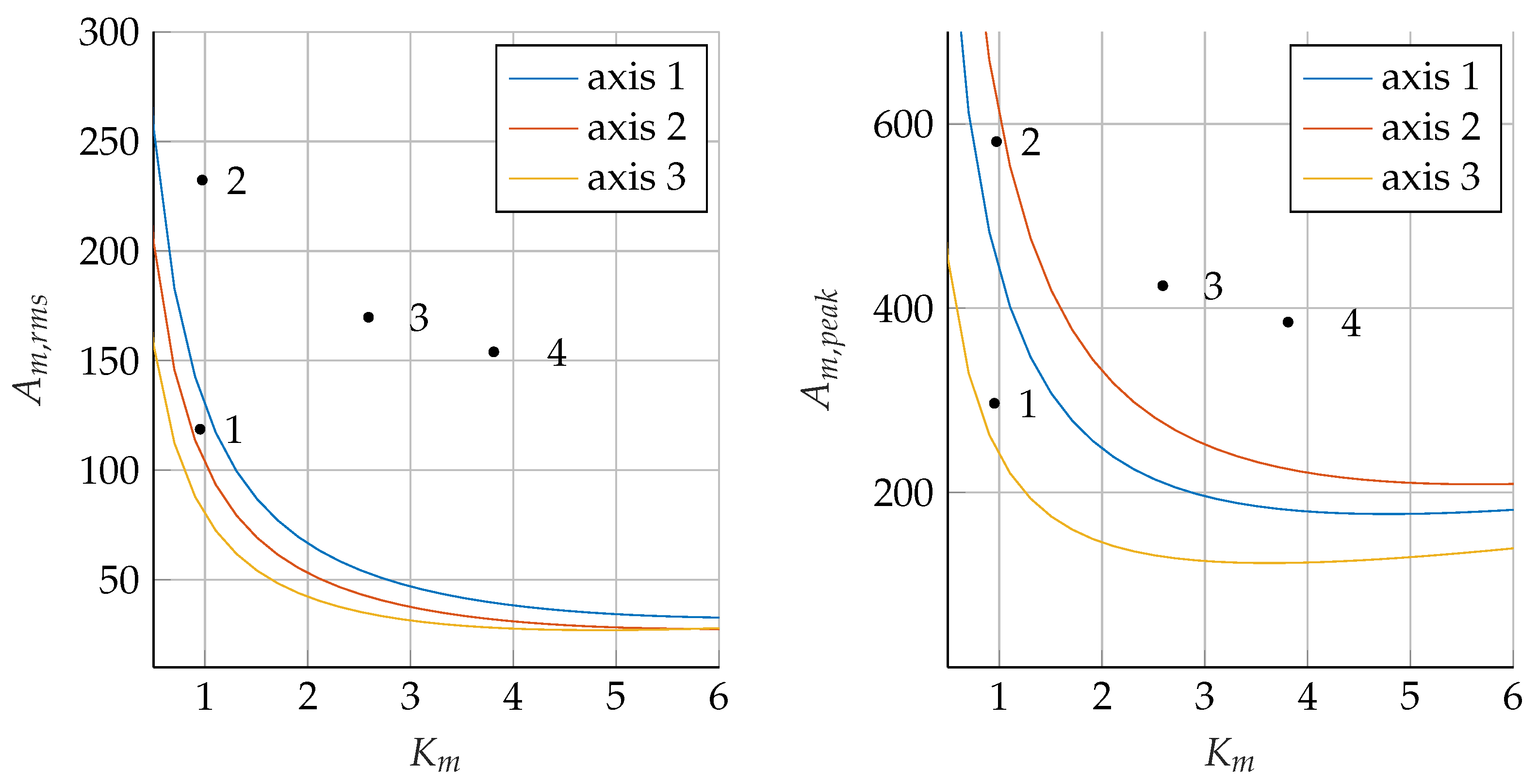
- The minimum point and the minimum value of ;
- The minimum point and the minimum value of ;
- The feasibility interval for a given drive system.
2.2. Sizing Procedure
- The load angular velocity at the output shaft ;
- The load angular acceleration at the output shaft ;
- The load torque at the output shaft ;
- One or more motors expressed as a pair of points ;
- For each motor, a list of practically matchable transmissions.
3. Case-Study Description
- Multiple degrees of freedom;
- Configuration-dependent and coupled inertial parameters;
- Mixed loads in which neither the dynamic actions nor the static contributions can be neglected.
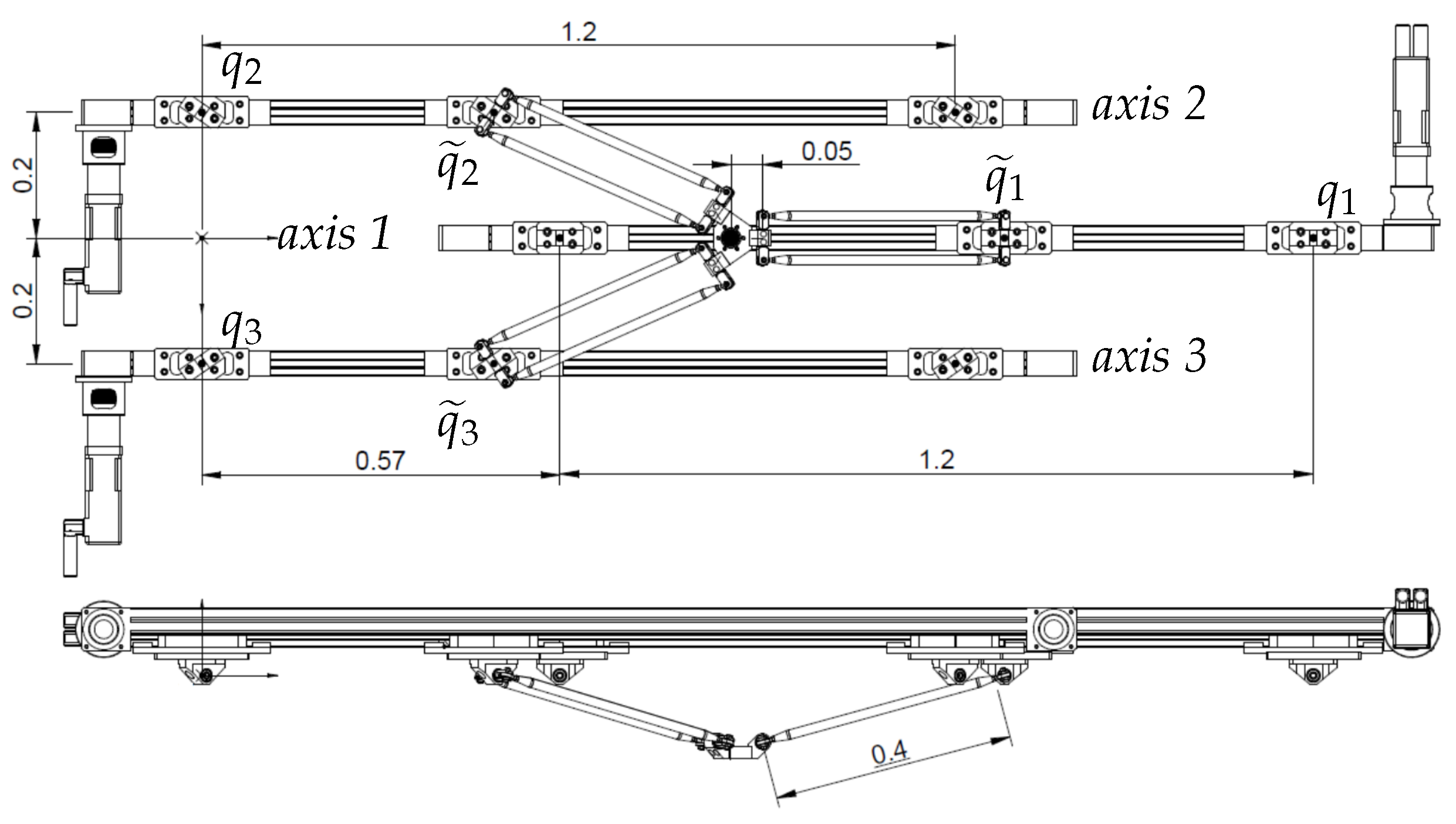
3.1. Mechanical Analysis
- The three linear axes are parallel to each other.
- Each linear axis is composed of a linear belt transmission, which is assumed to be stiff; the elements of vector represent the rotations of the actuated pulleys, which have radius ; is introduced to represent the translation of the carts.
- The motors will be connected to the actuated pulley of the linear belt transmission by means of a planetary transmission.
- The maximum axis stroke is 1.2 m.
- The distance between two consecutive axes is 200 mm.
- The length of the links connecting the carriages to the end effector is 400 mm.
- ,
- ,
- .
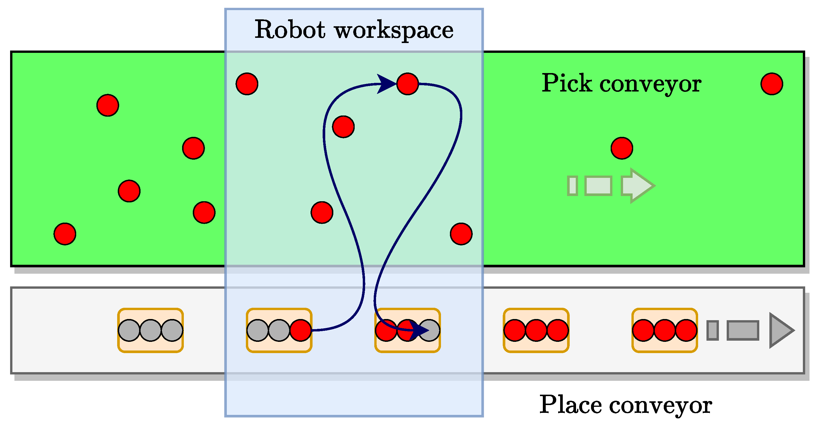
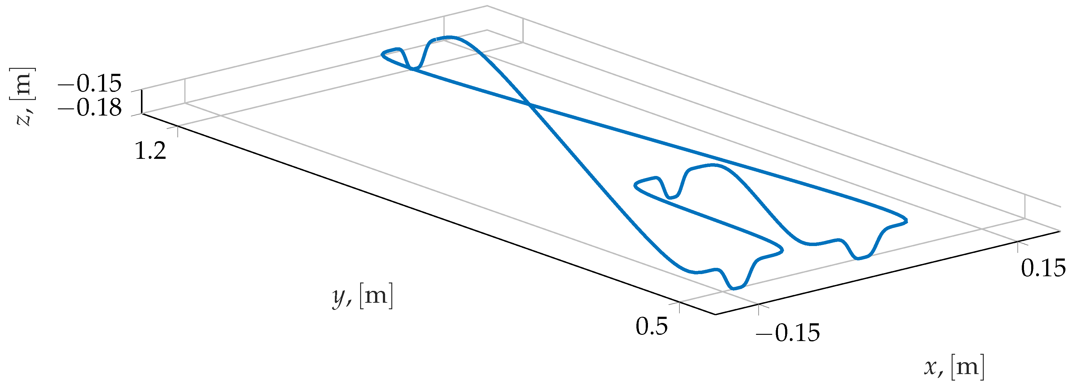
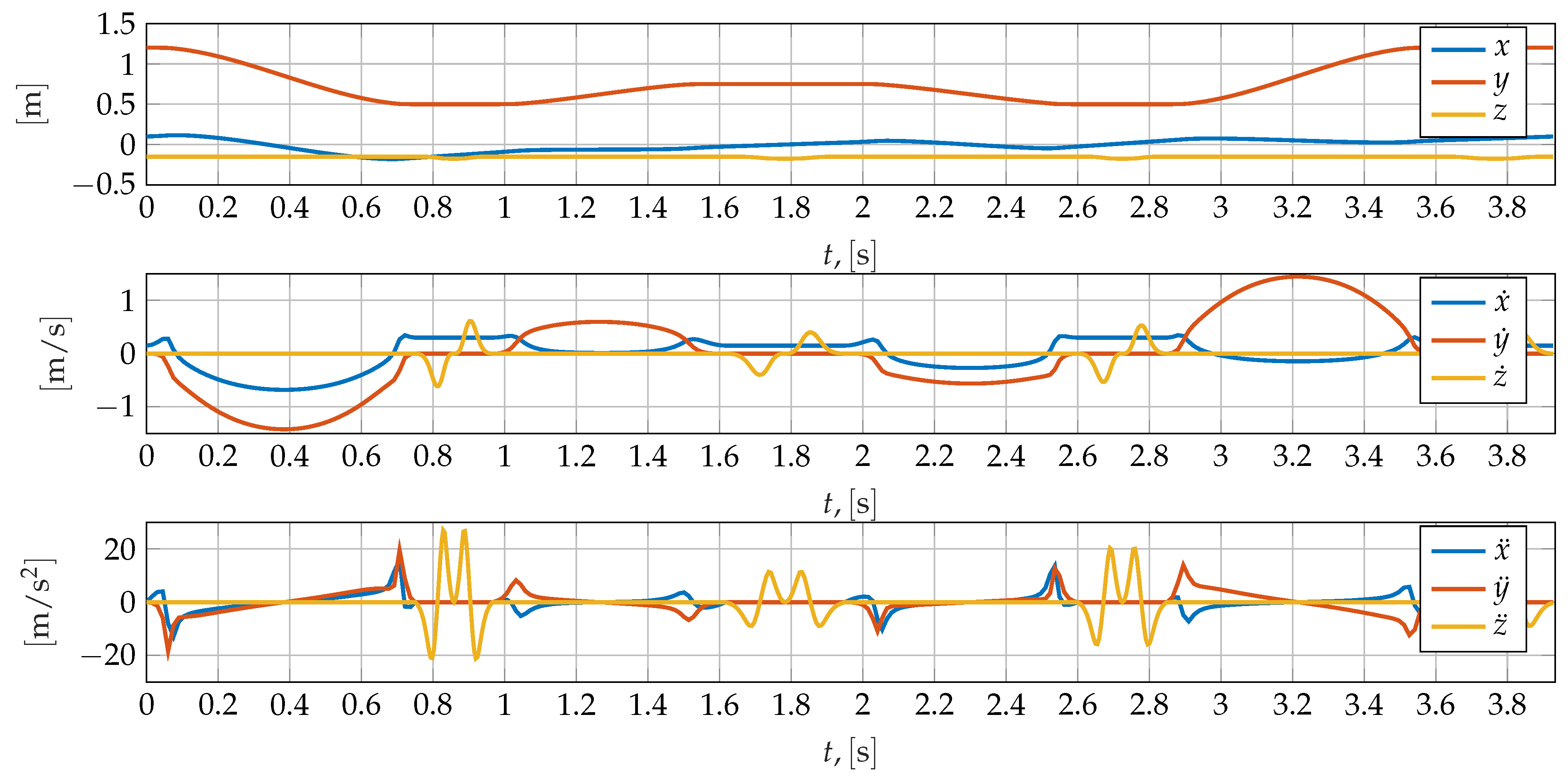
3.2. Work-Cycle Definition
4. Results and Discussion
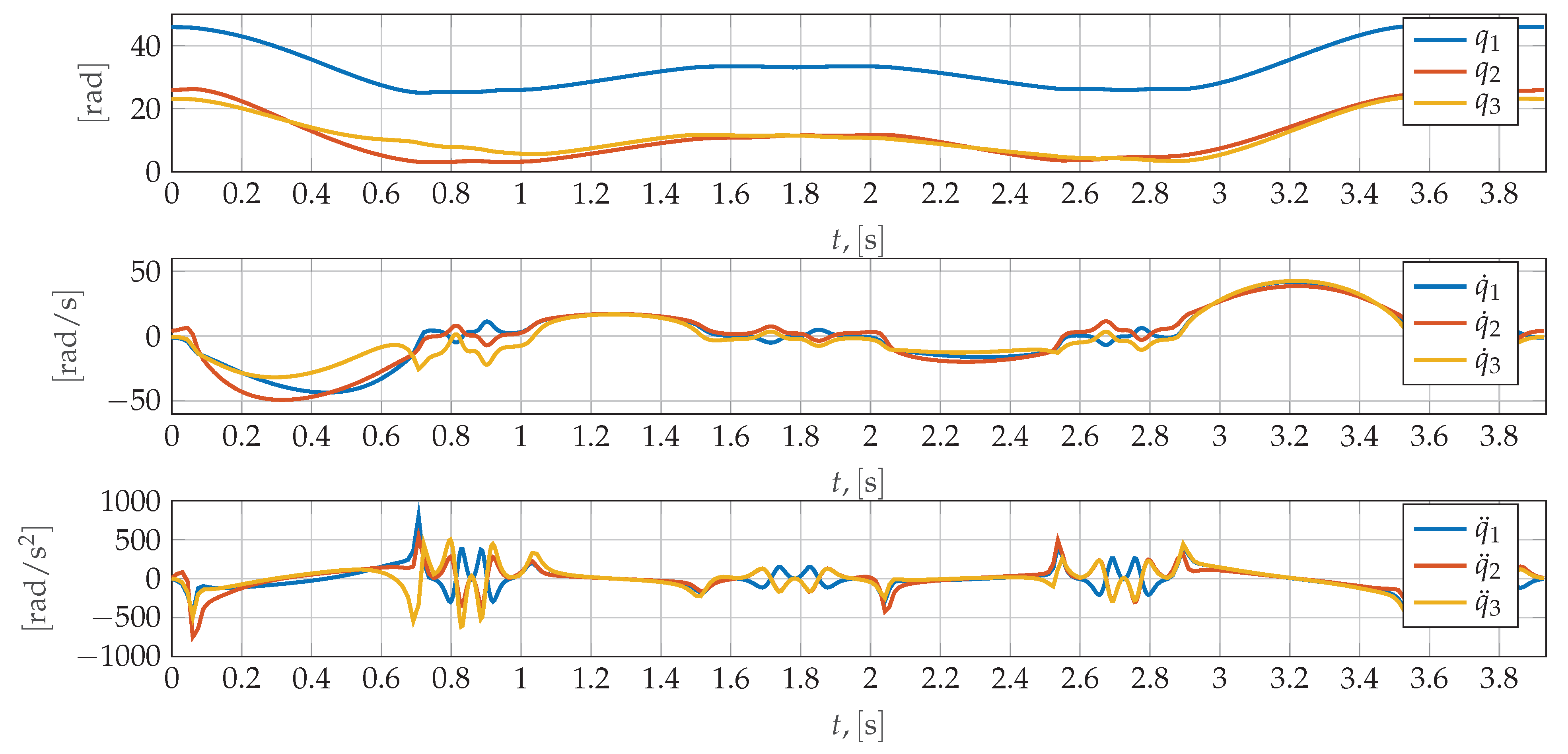
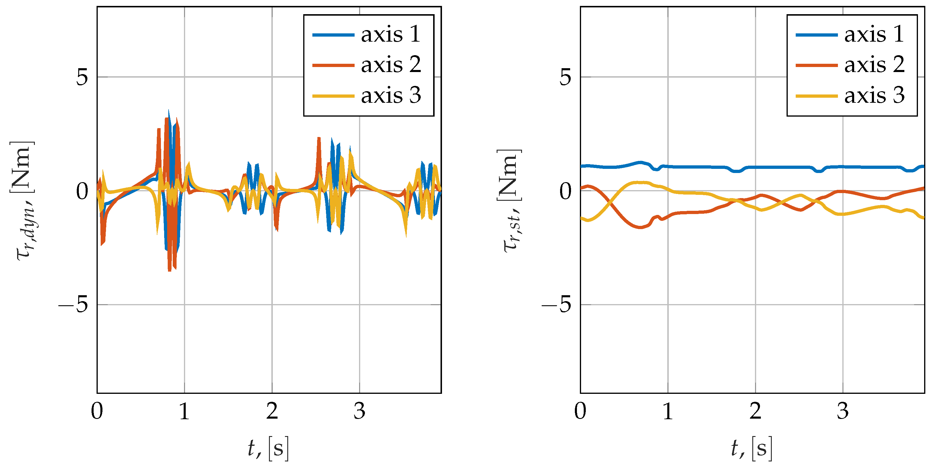
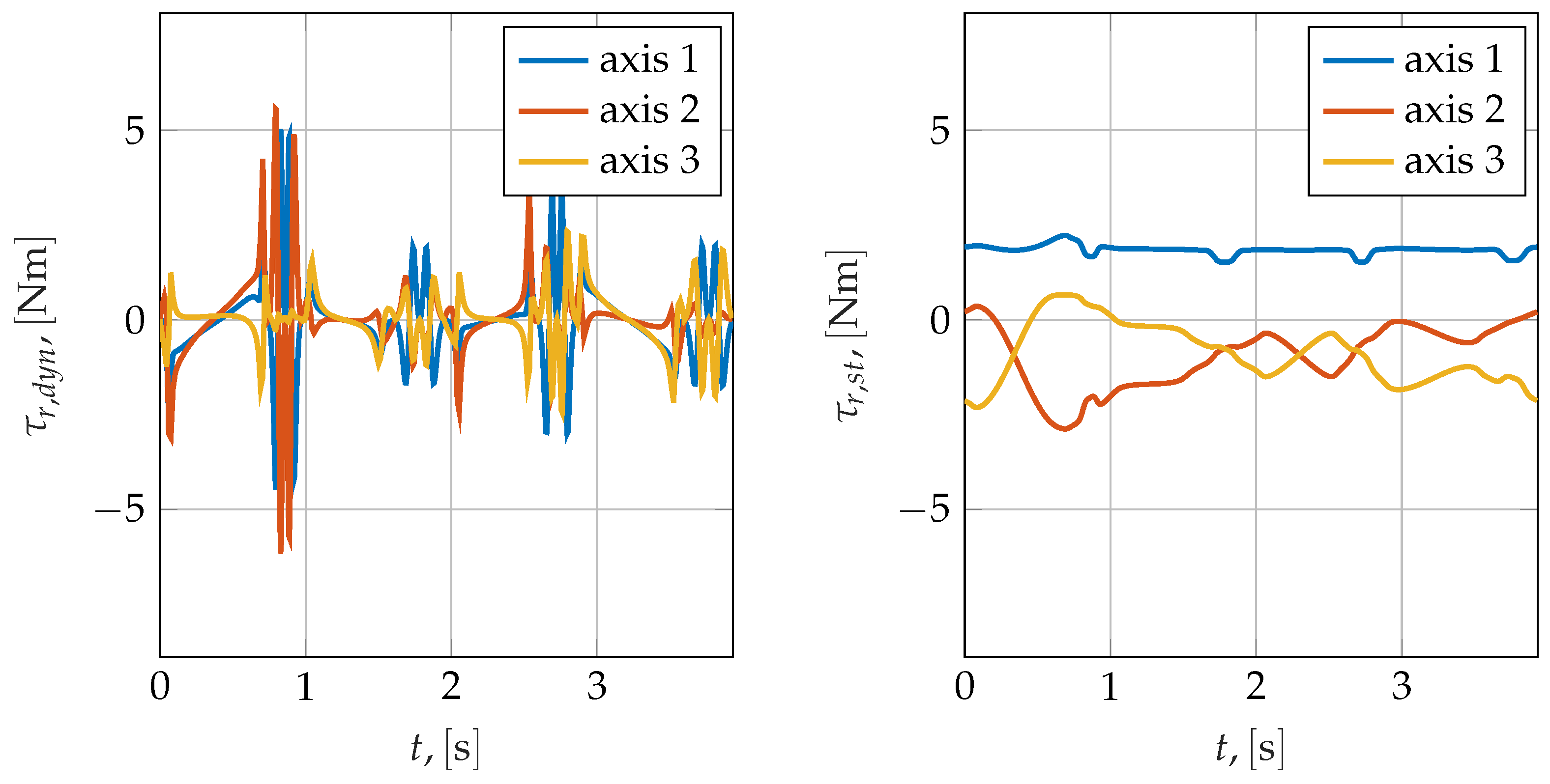
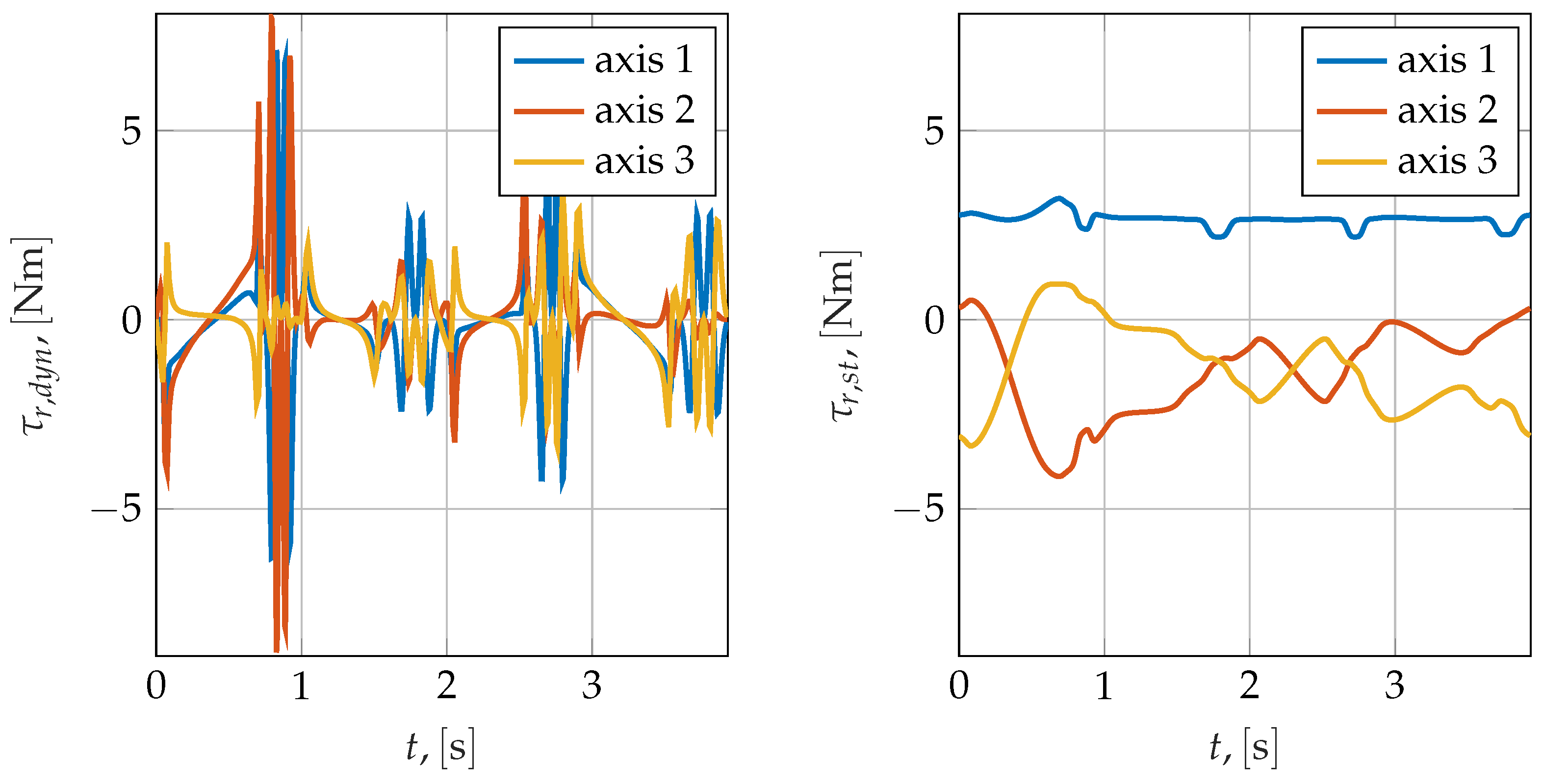
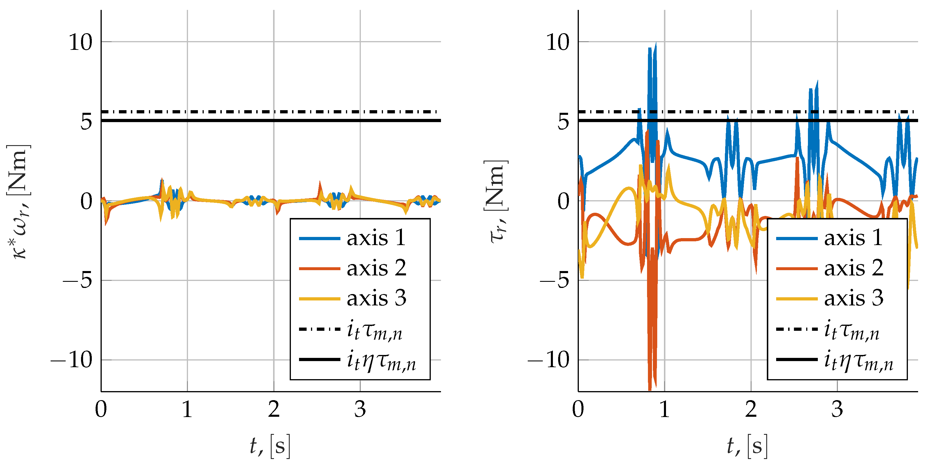
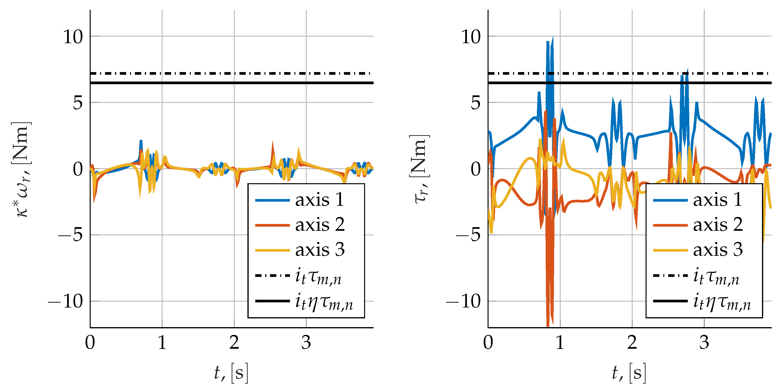
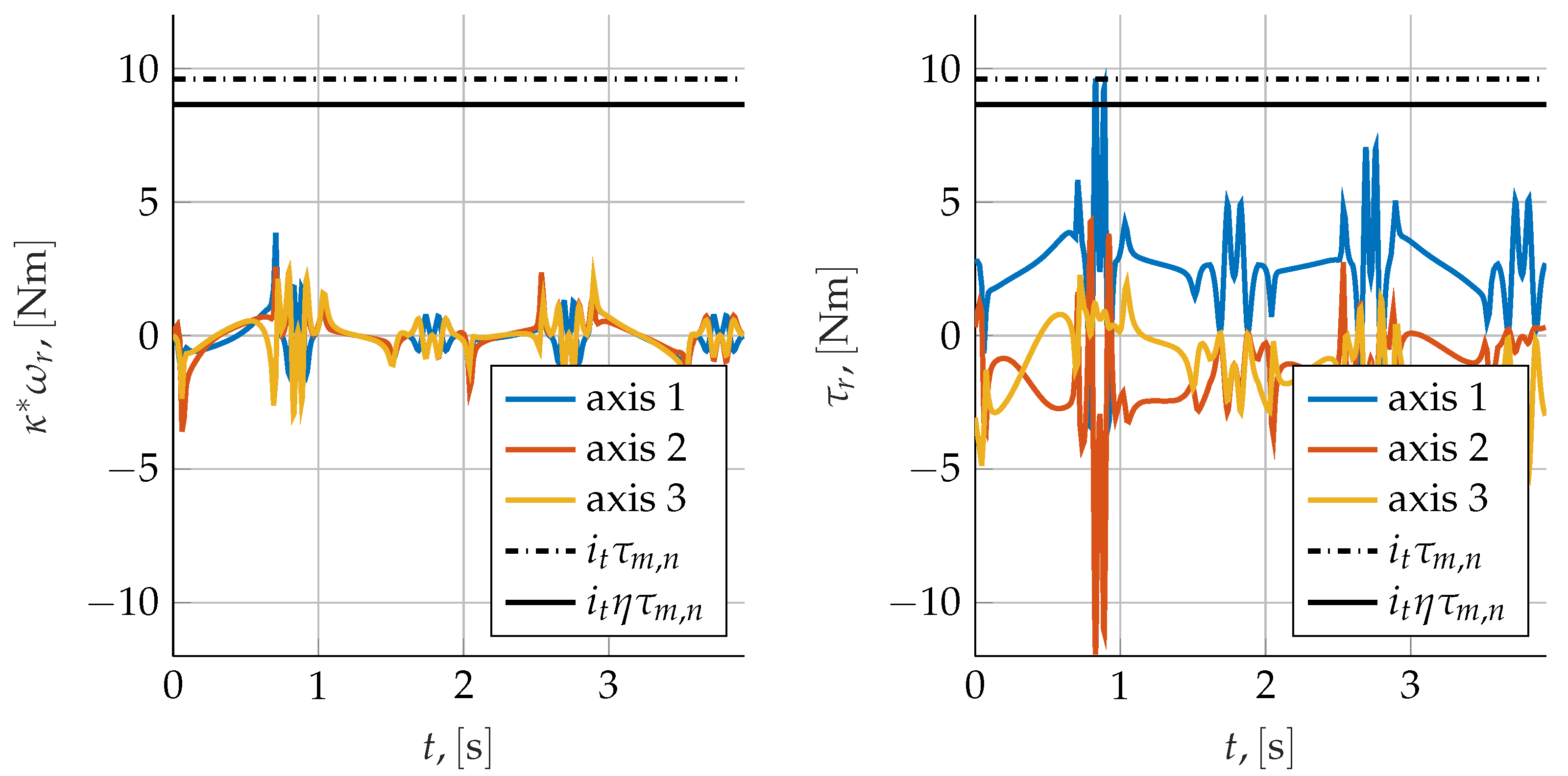
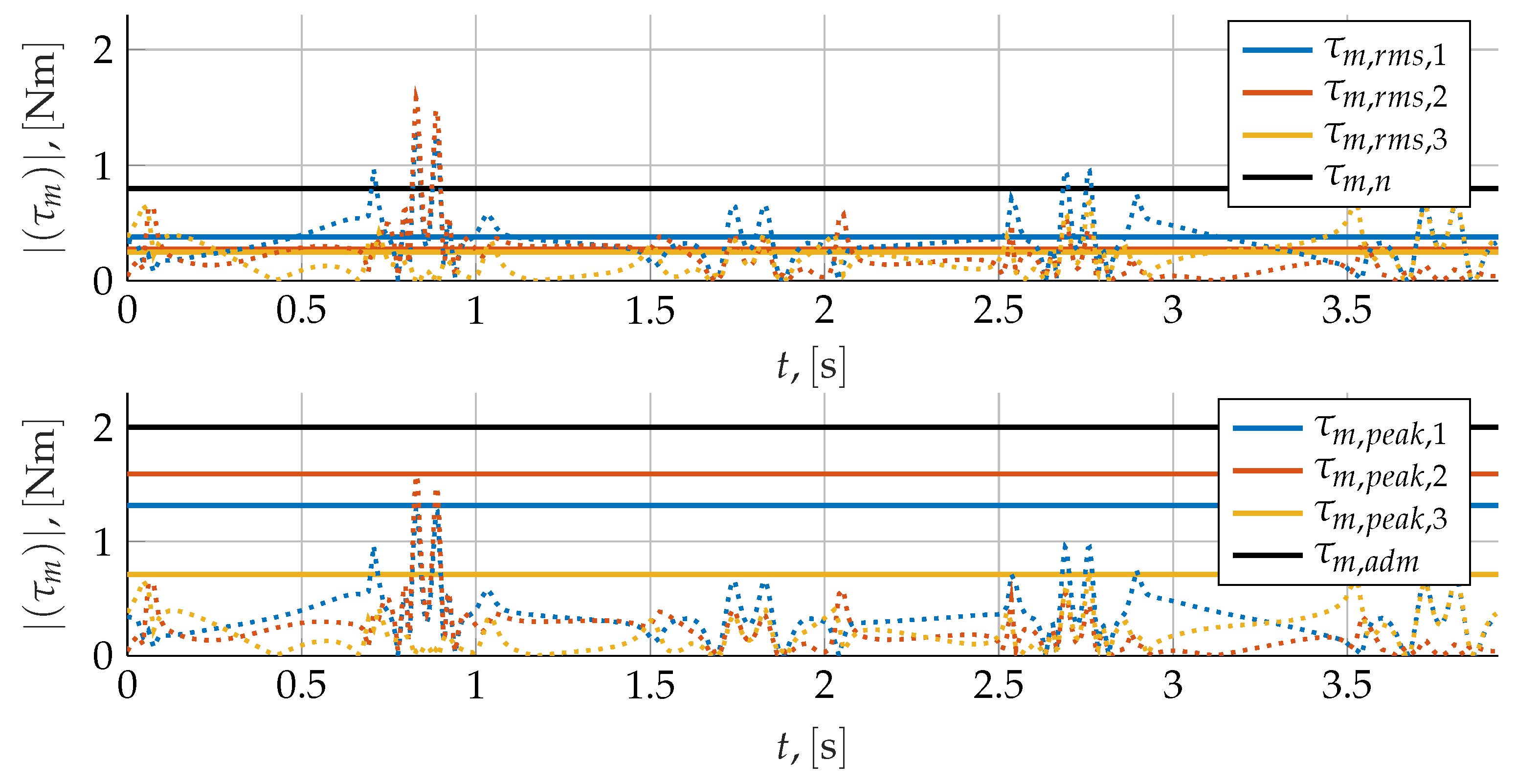
4.1. Time Domain Validation
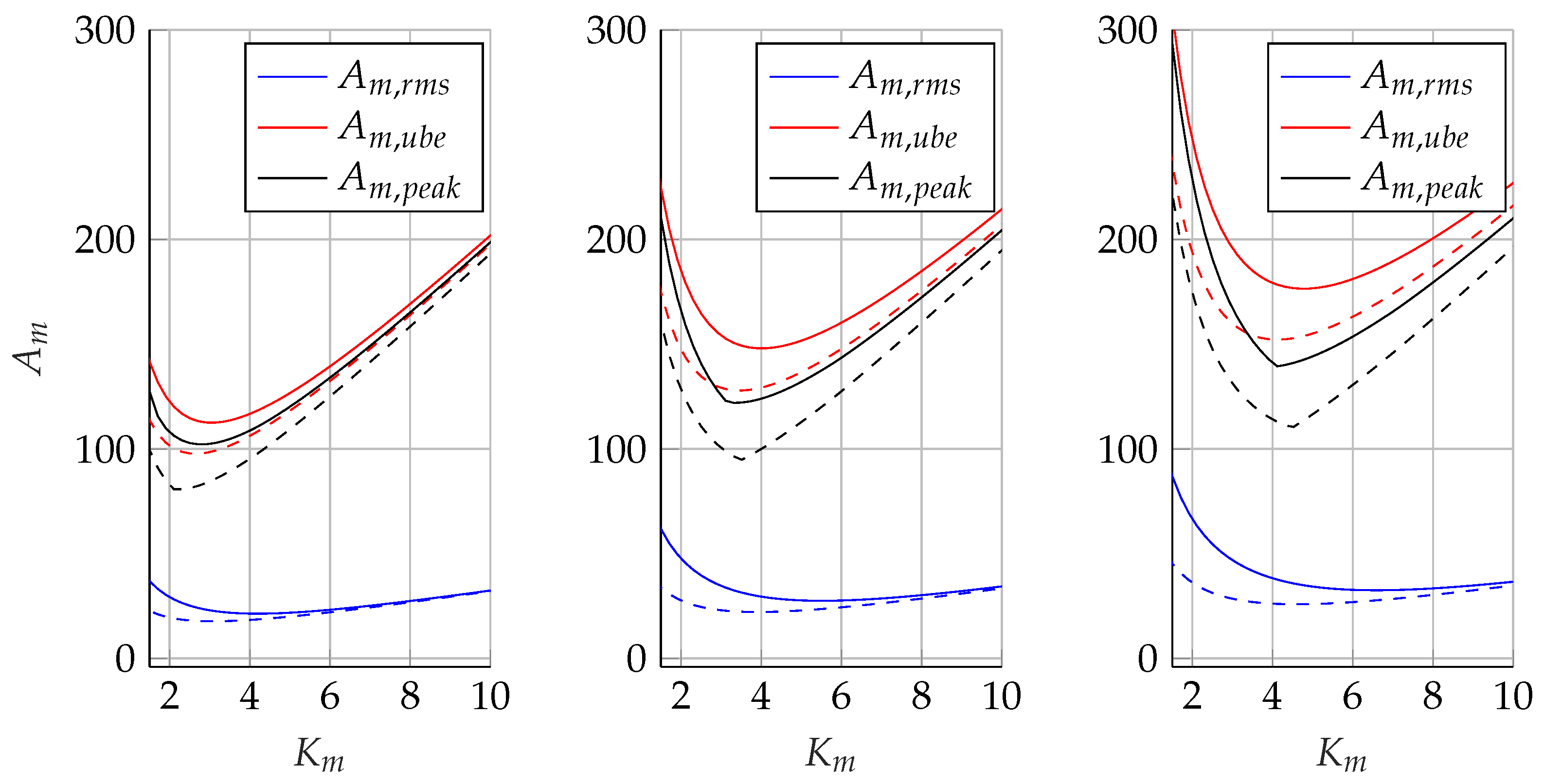
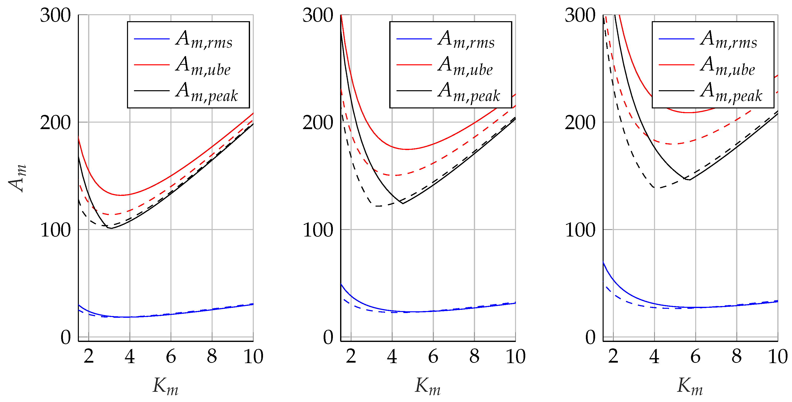
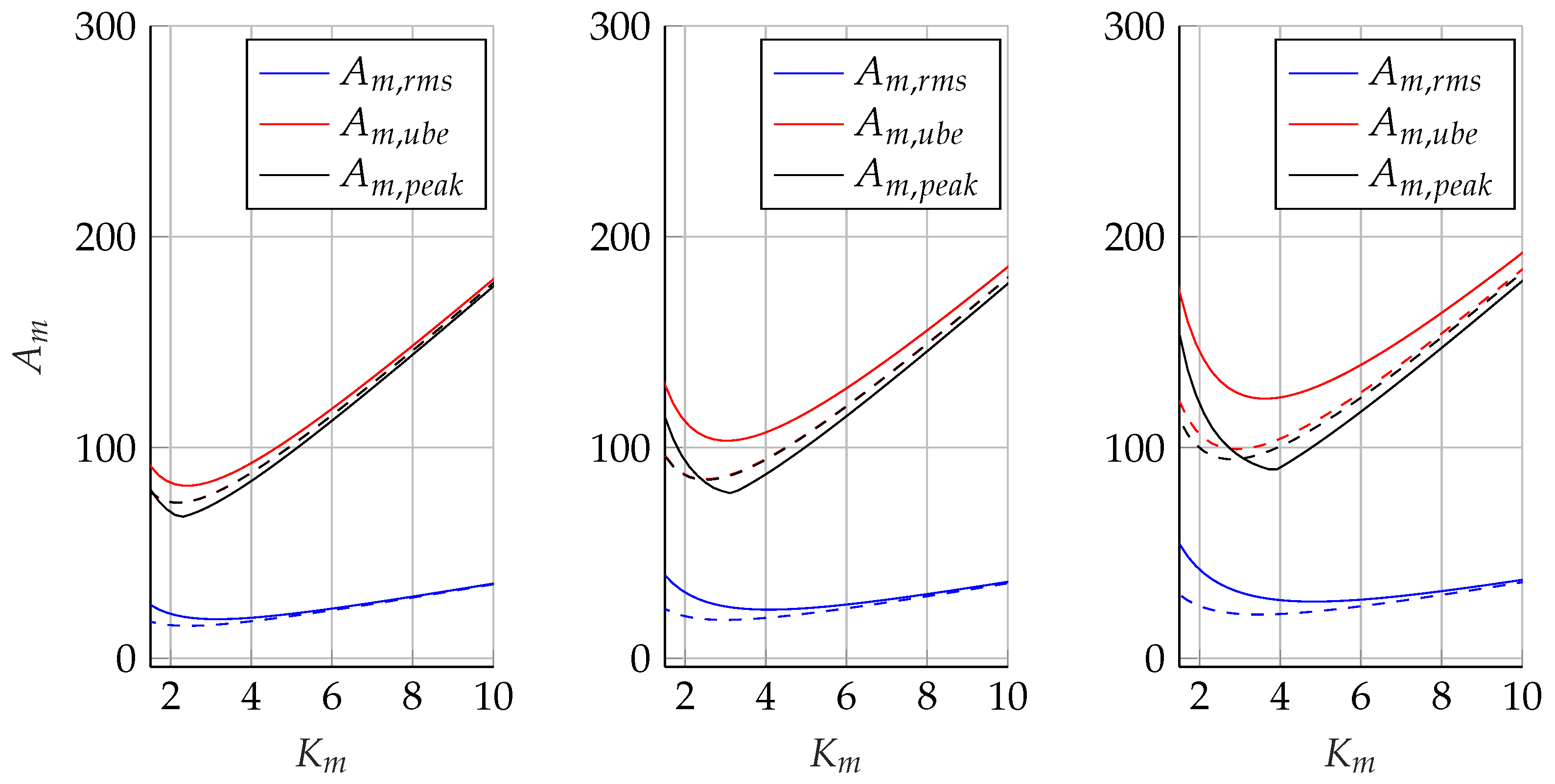
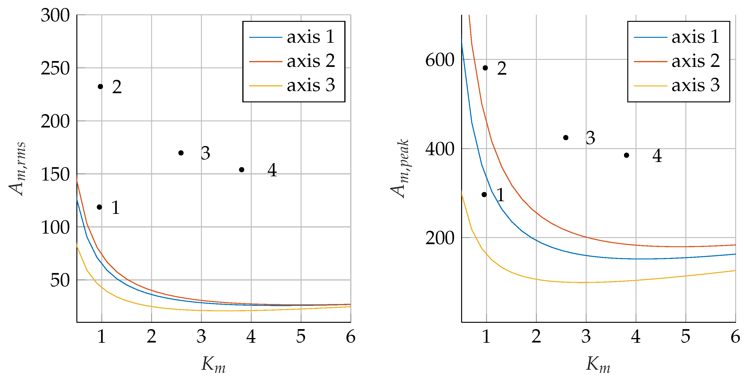
4.2. Purely Inertial Loading Conditions
5. Conclusions
Author Contributions
Funding
Institutional Review Board Statement
Informed Consent Statement
Data Availability Statement
Conflicts of Interest
Nomenclature
| Quantities related to the sizing procedure | |
| Accelerating factor at the motor shaft. | |
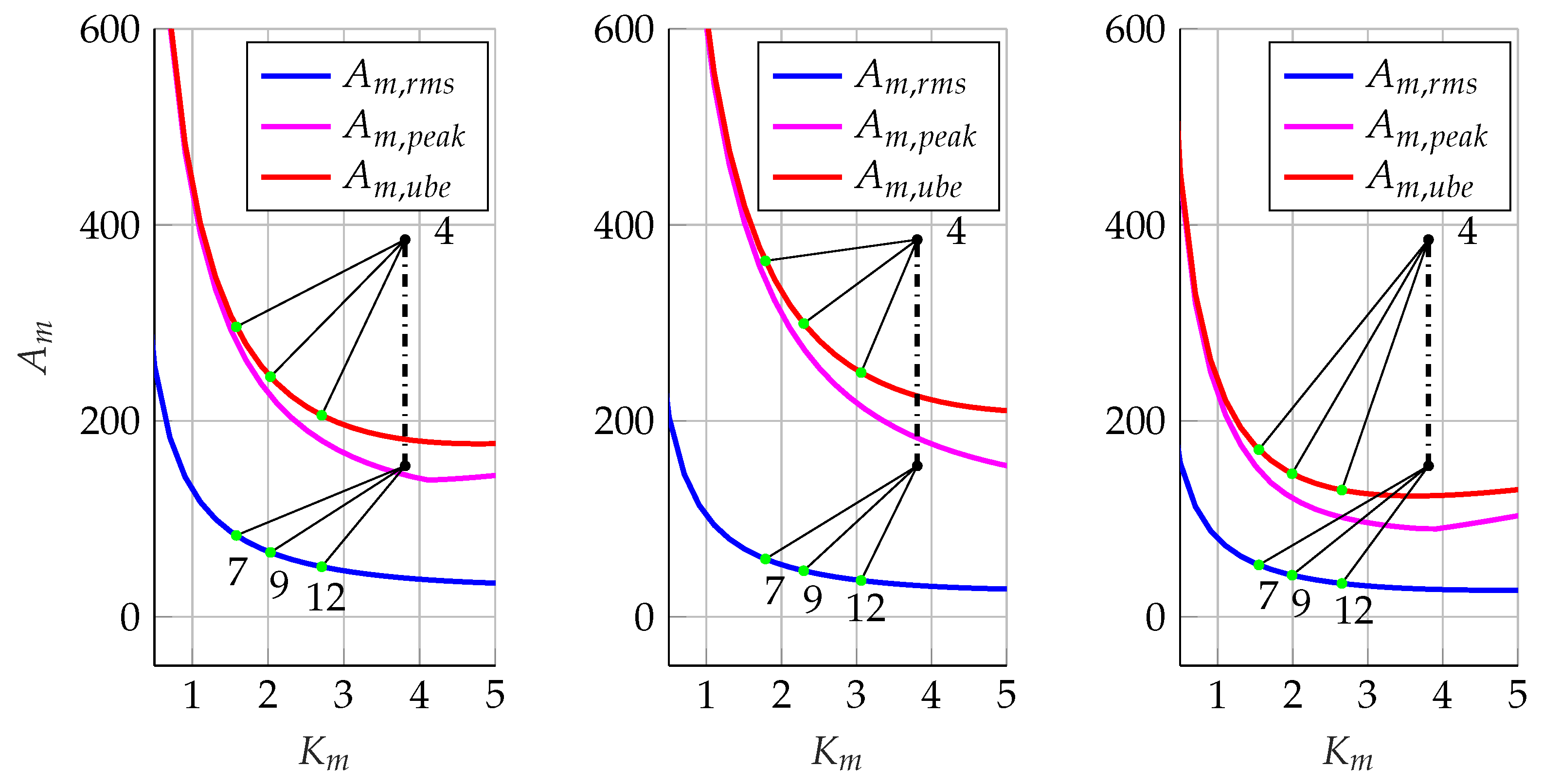
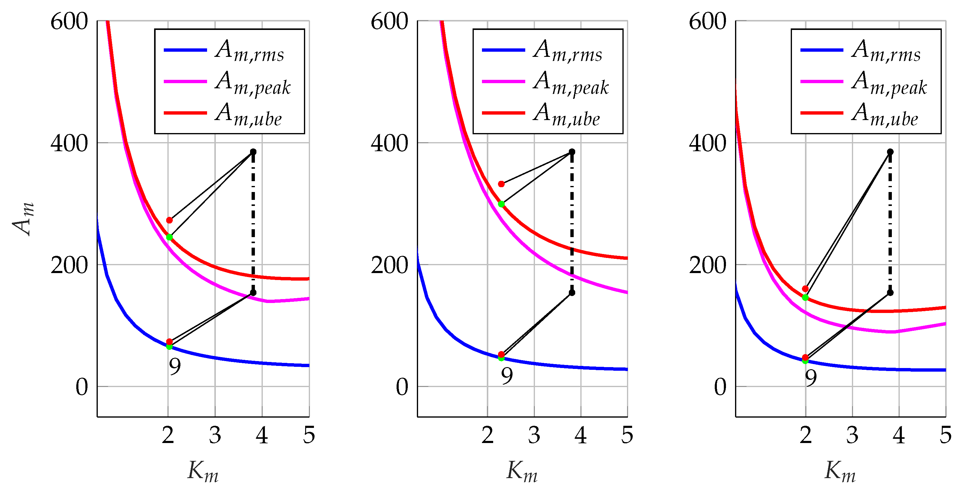
| Peak accelerating factor actually reached at the input shaft of the transmission. | |
| RMS accelerating factor reached at the input shaft of the transmission. | |
| Upper bound estimate of the peak accelerating factor reached at the input shaft of the transmission. | |
| Maximum admissible accelerating factor characterizing the power drive system. | |
| Rated accelerating factor of the power drive system. | |
| Efficiency of the transmission. | |
| Reduction ratio of the transmission. | |
| Inertia of the motor. | |
| Inertia of the transmission expressed at the input shaft. | |
| Kinetic factor at the motor shaft. | |
| Maximum admissible for a given PDS—load pair | |
| Minimum admissible for a given PDS—load pair | |
| Optimum kinetic factor minimizing the function. | |
| Optimum kinetic factor minimizing the function. | |
| Maximum admissible kinetic factor characterizing the power drive system. | |
| Integral average of the product . | |
| Peak torque safety margin. | |
| Rated torque safety margin. | |
| Safety margin related to the peak torque upper bound estimate. | |
| Peak velocity safety margin. | |
| Point in the plane characterizing the actual working conditions. | |
| Point in the plane characterizing the actual working conditions. | |
| Maximum admissible point in the plane characterizing the power drive system. | |
| Rated point in the plane characterizing the power drive system. | |
| Array collecting the positional coordinates of the mechanism’s actuated joints. | |
| Torque at the output shaft of the transmission. | |
| Peak torque actually reached at the output shaft of the transmission. | |
| RMS torque at the output shaft of the transmission. | |
| Torque at the input shaft of the transmission. | |
| Peak torque actually reached at the input shaft of the transmission. | |
| RMS torque at the input shaft of the transmission. | |
| Upper bound estimate of the torque required at the motor shaft. | |
| Maximum admissible torque characterizing the power drive system. | |
| Rated torque characterizing the power drive system. | |
| Execution time of the work cycle. | |
| Augmented load torque at the output shaft of the transmission. | |
| Angular velocity at the output shaft of the transmission. | |
| Angular acceleration at the output shaft of the transmission. | |
| RMS angular acceleration at the output shaft of the transmission. | |
| Peak angular velocity actually reached at the output shaft of the transmission. | |
| Peak angular acceleration actually reached at the output shaft of the transmission. | |
| Angular velocity at the input shaft of the transmission. | |
| Acceleration at the input shaft of the transmission. | |
| Peak angular velocity reached at the input shaft of the transmission. | |
| Maximum admissible angular velocity characterizing the power drive system. | |
| General Dynamic quantities | |
| Matrix of the Coriolis and centrifugal terms. | |
| Matrix of the viscous friction coefficients. | |
| g | Gravitational constant. |
| Mass matrix of the mechanical system. | |
| Array of the external generalized actions. | |
| Generalized external actions on the actuated joints. | |
| Gravitational potential energy. | |
| Gravitational potential. | |
| Quantities related to the applicative example | |
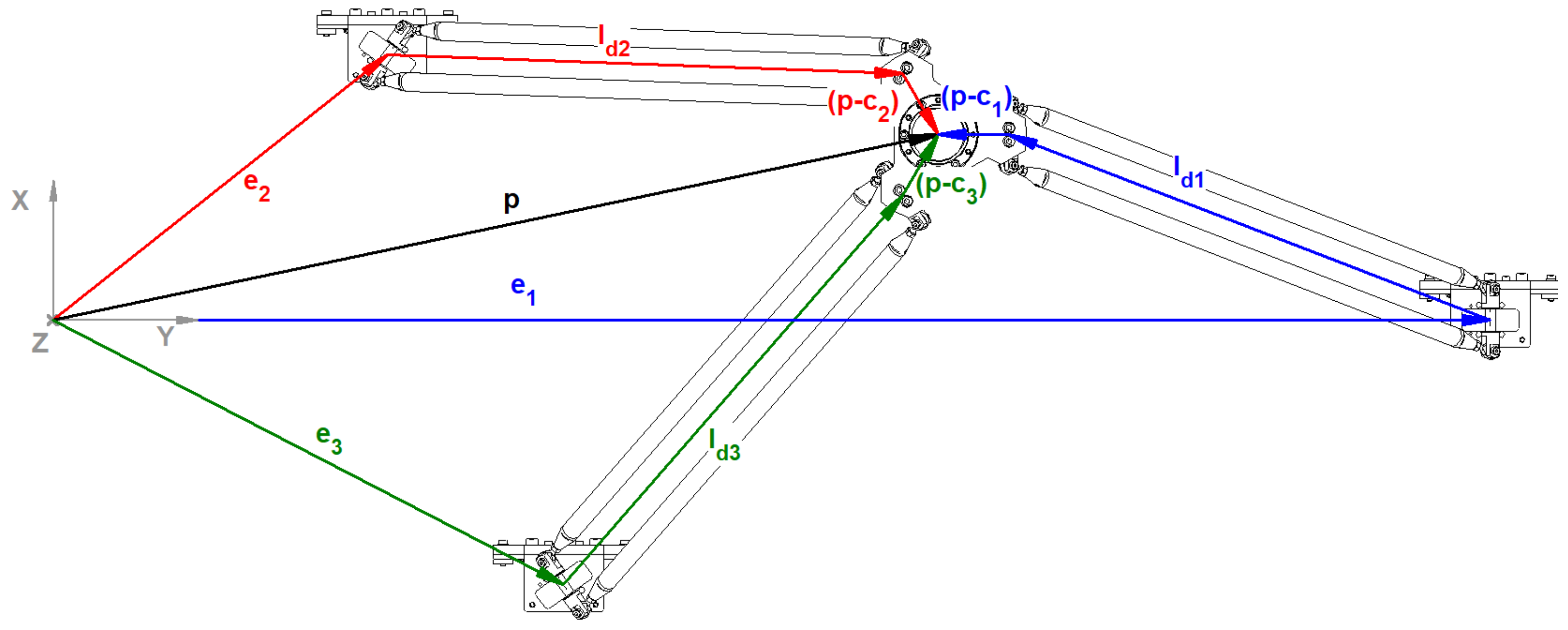
| Position of the constraint acting between the jthdistal linkage and the end-effector. | |
| Center of mass of the jthdistal link. | |
| Jacobian matrix associated to . | |
| Jacobian matrix associated to the jthtruck. | |
| Jacobian matrix associated to . | |
| Jacobian matrix associated to . | |
| Position of the jthtruck. | |
| Inertia tensor of the jthdistal link. | |
| Inertia tensor of the jthdistal link expressed in the principal barycentric frame. | |
| Length of the distal link. | |
| Vector pointing from the jthtruck to the jthplatform constraint. | |
| Distance between two consecutive linear guides of the linear delta robot. | |
| Mass of each distal link. | |
| Mass of the moving end-effector platform. | |
| Mass of each truck. | |
| Position of the end-effector platform. | |
| Coordinate describing the longitudinal position of the jthtruck. | |
| Array of the coordinates describing the longitudinal position of the three trucks. | |
| Array of the coordinates describing the longitudinal velocity of the three trucks. | |
| Array of the coordinates describing the longitudinal acceleration of the three trucks. | |
| Radius of the actuated and free pulleys. | |
| T | Kinetic energy of the mechanism. |
| Angular velocity of the jthdistal link. | |
References
- IEC 61800: 2021; Adjustable Speed Electrical Power Drive Systems. IEC: London, UK, 2021.
- Van De Straete, H.; Degezelle, P.; De Schutter, J.; Belmans, R. Servo motor selection criterion for mechatronic applications. IEEE/ASME Trans. Mechatron. 1998, 3, 43–50. [Google Scholar] [CrossRef]
- Van De Straete, H.; De Schutter, J.; Belmans, R. An efficient procedure for checking performance limits in servo drive selection and optimization. IEEE/ASME Trans. Mechatron. 1999, 4, 378–386. [Google Scholar] [CrossRef]
- Pasch, K.; Seering, W. On the drive systems for high—Performance machines. J. Mech. Des. Trans. ASME 1984, 106, 102–108. [Google Scholar] [CrossRef]
- Cusimano, G. A procedure for a suitable selection of laws of motion and electric drive systems under inertial loads. Mech. Mach. Theory 2003, 38, 519–533. [Google Scholar] [CrossRef]
- Cusimano, G. Generalization of a method for the selection of drive systems and transmissions under dynamic loads. Mech. Mach. Theory 2005, 40, 530–558. [Google Scholar] [CrossRef]
- Cusimano, G. Optimization of the choice of the system electric drive-device-transmission for mechatronic applications. Mech. Mach. Theory 2007, 42, 48–65. [Google Scholar] [CrossRef]
- Roos, F.; Johansson, H.; Wikander, J. Optimal selection of motor and gearhead in mechatronic applications. Mechatronics 2006, 16, 63–72. [Google Scholar] [CrossRef]
- Giberti, H.; Cinquemani, S.; Legnani, G. Effects of transmission mechanical characteristics on the choice of a motor-reducer. Mechatronics 2010, 20, 604–610. [Google Scholar] [CrossRef]
- Giberti, H.; Cinquemani, S.; Legnani, G. A practical approach to the selection of the motor-reducer unit in electric drive systems. Mech. Based Des. Struct. Mach. 2011, 39, 303–319. [Google Scholar] [CrossRef]
- Cusimano, G. Influence of the reducer efficiencies on the choice of motor and transmission: Torque peak of the motor. Mech. Mach. Theory 2013, 67, 122–151. [Google Scholar] [CrossRef]
- Cusimano, G. Choice of electrical motor and transmission in mechatronic applications: The torque peak. Mech. Mach. Theory 2011, 46, 1207–1235. [Google Scholar] [CrossRef]
- Cusimano, G. Choice of motor and transmission in mechatronic applications: Non-rectangular dynamic range of the drive system. Mech. Mach. Theory 2015, 85, 35–52. [Google Scholar] [CrossRef]
- Cusimano, G.; Casolo, F. An almost comprehensive approach for the choice of motor and transmission in mechatronics applications: Motor thermal problem. Mechatronics 2016, 40, 96–105. [Google Scholar] [CrossRef]
- Cusimano, G.; Casolo, F. An almost comprehensive approach for the choice of motor and transmission in mechatronic applications: Torque peak of the motor. Machines 2021, 9, 159. [Google Scholar] [CrossRef]
- Cusimano, G. Non-rectangular dynamic range of the drive system: A new approach for the choice of motor and transmission. Machines 2019, 7, 54. [Google Scholar] [CrossRef] [Green Version]
- Bartlett, H.; Lawson, B.; Goldfarb, M. Optimal transmission ratio selection for electric motor driven actuators with known output torque and motion trajectories. J. Dyn. Syst. Meas. Control Trans. ASME 2017, 139, 101013. [Google Scholar] [CrossRef]
- Meoni, F.; Carricato, M. Optimal selection of the motor-reducer unit in servo-controlled machinery: A continuous approach. Mechatronics 2018, 56, 132–145. [Google Scholar] [CrossRef]
- Aftab, Z.; Shafi, F.; Shad, R.; Inzimam-Ul-Haq, R.; Saeed, K. Systematic method for selection of motor-reducer units to power a lower-body robotic exoskeleton. J. Appl. Sci. Eng. (Taiwan) 2021, 24, 457–465. [Google Scholar] [CrossRef]
- Campolo, D. Motor selection via impedance-matching for driving nonlinearly damped, resonant loads. Mechatronics 2010, 20, 566–573. [Google Scholar] [CrossRef]
- Giberti, H.; Cinquemani, S.; Ambrosetti, S. 5R 2dof parallel kinematic manipulator—A multidisciplinary test case in mechatronics. Mechatronics 2013, 23, 949–959. [Google Scholar] [CrossRef]
- Han, G.; Xie, F.; Liu, X.J. Optimal selection of servo motor and reduction ratio for high-speed parallel robots. In Lecture Notes in Computer Science (Including Subseries Lecture Notes in Artificial Intelligence and Lecture Notes in Bioinformatics); Springer: Cham, Switzerland, 2015; Volume 9245, pp. 109–120. [Google Scholar] [CrossRef]
- Ge, L.; Chen, J.; Li, R.; Liang, P. Optimization design of drive system for industrial robots based on dynamic performance. Ind. Robot. 2017, 44, 765–775. [Google Scholar] [CrossRef]
- Padilla-Garcia, E.; Cruz-Villar, C.; Rodriguez-Angeles, A.; Moreno-Armendáriz, M. Concurrent optimization on the powertrain of robot manipulators for optimal motor selection and control in a point-to-point trajectory planning. Adv. Mech. Eng. 2017, 9, 1687814017747368. [Google Scholar] [CrossRef] [Green Version]
- Xie, Z.; Xie, F.; Liu, X.J.; Wang, J.; Shen, X. Parameter optimization for the driving system of a 5 degrees-of-freedom parallel machining robot with planar kinematic chains. J. Mech. Robot. 2019, 11, 041003. [Google Scholar] [CrossRef]
- Barjuei, E.; Ardakani, M.; Caldwell, D.; Sanguineti, M.; Ortiz, J. Optimal Selection of Motors and Transmissions in Back-Support Exoskeleton Applications. IEEE Trans. Med. Robot. Bion. 2020, 2, 320–330. [Google Scholar] [CrossRef]
- Huang, T.; Mei, J.; Li, Z.; Zhao, X.; Chetwynd, D. A method for estimating servomotor parameters of a parallel robot for rapid pick-and-place operations. J. Mech. Des. Trans. ASME 2005, 127, 596–601. [Google Scholar] [CrossRef]
- Shao, Z.; Tang, X.; Chen, X.; Wang, L. Inertia match of a 3-RRR reconfigurable planar parallel manipulator. Chin. J. Mech. Eng. (Engl. Ed.) 2009, 22, 791–799. [Google Scholar] [CrossRef]
- Liu, Z.; Tang, X.; Shao, Z.; Wang, L. Dimensional optimization of the Stewart platform based on inertia decoupling characteristic. Robotica 2016, 34, 1151–1167. [Google Scholar] [CrossRef]
- Kong, Y.; Cheng, G.; Guo, F.; Gu, W.; Zhang, L. Inertia matching analysis of a 5-DOF hybrid optical machining manipulator. J. Mech. Sci. Technol. 2019, 33, 4991–5002. [Google Scholar] [CrossRef]
- Righettini, P.; Strada, R.; Remuzzi, A. A mechatronic apparatus for shear stress application on endothelial cells: Design, development and experimental tests. In Proceedings of the 2021 IEEE International Conference on Mechatronics, Kashiwa, Japan, 7–9 March 2021. [Google Scholar] [CrossRef]
- Righettini, P.; Strada, R.; Zappa, B.; Lorenzi, V. Experimental set-up for the investigation of transmissions effects on the dynamic performances of a linear PKM. Mech. Mach. Sci. 2019, 73, 2511–2520. [Google Scholar] [CrossRef]
- Righettini, P.; Strada, R.; Cortinovis, F. Modal kinematic analysis of a parallel kinematic robot with low-stiffness transmissions. Robotics 2021, 10, 132. [Google Scholar] [CrossRef]
- Clavel, R. Delta, a fast robot with parallel geometry. In Proceedings of the 1988 IEEE International Symposium on Industrial Robot, Philadelphia, PA, USA, 28–29 April 1988. [Google Scholar]
- Voglewede, P.; Ebert-Uphoff, I. Overarching framework for measuring closeness to singularities of parallel manipulators. IEEE Trans. Robot. 2005, 21, 1037–1045. [Google Scholar] [CrossRef]
- Laryushkin, P.; Glazunov, V.; Erastova, K. On the Maximization of Joint Velocities and Generalized Reactions in the Workspace and Singularity Analysis of Parallel Mechanisms. Robotica 2019, 37, 675–690. [Google Scholar] [CrossRef]


| Type | Ta, [s] | P0, [m] | Pf, [m] |
|---|---|---|---|
| Place | 0.97 | ( 0.100; 1.200; −0.150) | (−0.100; 0.500; −0.150) |
| Pick | 0.98 | (−0.100; 0.500; −0.150) | ( 0.025; 0.750; −0.150) |
| Place | 0.90 | ( 0.025; 0.750; −0.150) | ( 0.050; 0.500; −0.150) |
| Pick | 1.08 | ( 0.050; 0.500; −0.150) | ( 0.100; 1.200; −0.150) |
| ID | , [kg m2] | , [V] | , [rad/s] | , [N m] | , [N m] | |||
|---|---|---|---|---|---|---|---|---|
| 1 | 2.30 | 220 | 628.3 | 0.18 | 0.45 | 0.95 | 118.7 | 296.7 |
| 2 | 2.40 | 220 | 628.3 | 0.36 | 0.90 | 0.97 | 232.4 | 580.9 |
| 3 | 1.70 | 220 | 628.3 | 0.70 | 1.75 | 2.59 | 169.8 | 424.4 |
| 4 | 2.70 | 220 | 733.0 | 0.80 | 2.00 | 3.81 | 154.0 | 384.9 |
| 5 | 5.10 | 220 | 628.3 | 1.90 | 4.75 | 4.49 | 266.1 | 665.1 |
| B | ||||||||
|---|---|---|---|---|---|---|---|---|
| Axis 1 | 1.88 | 1.88 | 2.35 | 2.10 | 1.71 | 1.52 | 1.57 | 1.41 |
| Axis 2 | 1.66 | 1.66 | 3.28 | 2.93 | 1.41 | 1.26 | 1.29 | 1.16 |
| Axis 3 | 1.91 | 1.91 | 3.63 | 3.24 | 3.17 | 2.81 | 2.64 | 2.40 |
Publisher’s Note: MDPI stays neutral with regard to jurisdictional claims in published maps and institutional affiliations. |
© 2022 by the authors. Licensee MDPI, Basel, Switzerland. This article is an open access article distributed under the terms and conditions of the Creative Commons Attribution (CC BY) license (https://creativecommons.org/licenses/by/4.0/).
Share and Cite
Righettini, P.; Strada, R.; Cortinovis, F. General Procedure for Servo-Axis Design in Multi-Degree-of-Freedom Machinery Subject to Mixed Loads. Machines 2022, 10, 454. https://doi.org/10.3390/machines10060454
Righettini P, Strada R, Cortinovis F. General Procedure for Servo-Axis Design in Multi-Degree-of-Freedom Machinery Subject to Mixed Loads. Machines. 2022; 10(6):454. https://doi.org/10.3390/machines10060454
Chicago/Turabian StyleRighettini, Paolo, Roberto Strada, and Filippo Cortinovis. 2022. "General Procedure for Servo-Axis Design in Multi-Degree-of-Freedom Machinery Subject to Mixed Loads" Machines 10, no. 6: 454. https://doi.org/10.3390/machines10060454