Kinematic and Dynamic Modeling and Workspace Analysis of a Suspended Cable-Driven Parallel Robot for Schönflies Motions

Abstract

In recent years, cable-driven parallel robots (CDPRs) have drawn more and more attention due to the properties of large workspace, large payload capacity, and ease of reconfiguration. In this paper, we present a kinematic and dynamic modeling and workspace analysis for a novel suspended CDPR which generates Schönflies motions. Firstly, the architecture of the robot is introduced, and the inverse and forward kinematic problems of the robot are solved through a geometrical approach. Then, the dynamic equation of the robot is derived by separately considering the moving platform and the drive trains. Based on the dynamic equation, the dynamic feasible workspace of the robot is determined under different values of accelerations. Finally, experiments are performed on a prototype of the robot to demonstrate the correctness of the derived models and workspace.

1. Introduction

Cable-driven parallel robots (CDPRs) are particular types of parallel robots in which the rigid kinematic chains are replaced by flexible cables [1]. In recent years, CDPRs have drawn more and more attention due to the properties of large workspace, large payload capacity, and ease of reconfiguration [2,3]. CDPRs are divided into the suspended type and the fully constrained type according to the tensioning methods. For the suspended CDPRs, the cables are all located over the moving platform, and the gravity of the moving platform is essential to keep the cables in tension. Since the space below the moving platform is free of cables, the suspended CDPRs are generally used to obtain a large workspace. The suspended CDPRs usually work under static conditions because of the limited gravity [4]. For the fully constrained CDPRs, the cables are located on both sides of the moving platform and pull against each other to ensure positive cable tensions. The fully constrained CDPRs are suitable to generate high-speed motions with large accelerations [5].

The existence of the flexible cables greatly complicates the modeling and analysis of CDPRs. On the one hand, the elasticity of the cables leads to low stiffness and deteriorates the positioning accuracy of CDPRs. On the other hand, resulting from the unilateral property, the cables can only apply pull forces and cannot provide push forces. Thus, a greater number of cables than the degrees of freedom (DOFs) are generally required to fully control CDPRs [6]. Many recent works have contributed to the modeling and analysis of CDPRs. In [7], the authors present the kinetostatic model of a 3-DOF CDPR involving pulley kinematics and cable elasticity. Meanwhile, a novel pulley structure is proposed to improve the positioning accuracy of CDPRs. The kinematic model of CDPRs considering pulley mechanisms is presented in [8]. Based on the kinematic model, a kinematic calibration method is further developed for CDPRs. In [9], the forward kinetostatic problem of a 6-DOF underactuated CDPR is solved using an unsupervised neural network approach. This novel approach is computationally efficient and has an accuracy similar to that of other optimization methods. In [10], the authors provide a kinematic and dynamic analysis of a CDPR composed of multiple cranes by considering the hydraulic actuation system. A 3-DOF CDPR driven by five-bar winding mechanisms for workspace expansion is presented in [11]. The kinematic and dynamic analysis of the CDPR is performed based on the finite element method and the Lagrange formulation. In [12], the dynamic model of CDPRs is derived by combining the finite element model of the cables with the rigid-body dynamics of the moving platform.

Another important issue is determining the workspace of CDPRs, as the workspace is one of the decisive properties for the potential applications of CDPRs. The workspace of CDPRs is strongly coupled to the cable tensions because of the unilateral property of the cables [13]. A generalized ray-based method is proposed in [14] to solve the wrench-closure workspace of CDPRs. The authors further introduce a graph representation to visualize the high-dimensional workspace. In [15], the wrench-feasible workspace of CDPRs is computed through interval analysis, in which the sets fully inside or outside the workspace can be efficiently determined. The dynamic feasible workspace of a 6-DOF CDPR is solved by investigating the dynamic equilibrium of the moving platform in [16]. The authors in [17,18] use a geometric method to calculate the cylindrical operation workspace of a 3-DOF CDPR tensioned by passive springs. The relation between the number of springs and the shape of the workspace is investigated. In [19], a geometric approach based on convex analysis is proposed to compute the workspace of CDPRs subject to the constraints of the cable tensions. In [20], the author proposes the differential workspace hull method to calculate the workspace of CDPRs. This method adopts a triangulation representation to approximate the boundary of the workspace and can handle various criteria for the workspace.

Although much effort has been devoted to the modeling and analysis of CDPRs, the existing works mainly focus on the purely translational 3-DOF CDPRs [7,11,17,18] and the spatial 6-DOF CDPRs [9,12,16,20]. The CDPRs with other types of motions have seldom been reported, and there is no systematic approach for the modeling and analysis of such kinds of CDPRs. In many working scenarios, not all directions of motions are essential for the application requirements, and the redundant DOFs may increase the cost and complicate the robot systems [21]. Therefore, there is an urgent need to investigate the lower-mobility CDPRs with sub-spatial motions. Among the lower-mobility motion types, Schönflies motion, which contains three-dimensional translation and one-dimensional rotation about the vertical axis, is the most widely used kind of sub-spatial motion in robotics [22]. Aiming to narrow the research gap and complement the field of lower-mobility CDPRs, in this paper, we present a kinematic and dynamic modeling and workspace analysis for a novel suspended CDPR which generates Schönflies motions. In comparison with the existing works, the main contributions of this paper are summarized as follows:

• The structure of the novel CDPR which generates Schönflies motions is introduced to complement the field of lower-mobility CDPRs.
• The closed-form solutions for the inverse and forward kinematics of the robot are derived based on a geometrical approach.
• The dynamic model of the robot is formulated based on the virtual power principle, which lays the foundation for the workspace determination and the model-based control of the robot.
• The dynamic feasible workspace of the robot is determined under different values of accelerations, which facilitates the motion planning and control of the robot.

The remaining parts of this paper are arranged as follows. The architecture of the novel CDPR is introduced in Section 2. Then, the inverse and forward kinematic problems of the robot are solved in Section 3. Section 4 presents the dynamic modeling of the robot by separately considering the moving platform and the drive trains. Section 5 determines the dynamic feasible workspace of the robot under different values of accelerations. The prototype and experiments of the robot are presented in Section 6. Finally, Section 7 concludes this paper and discusses suggestions for future work.

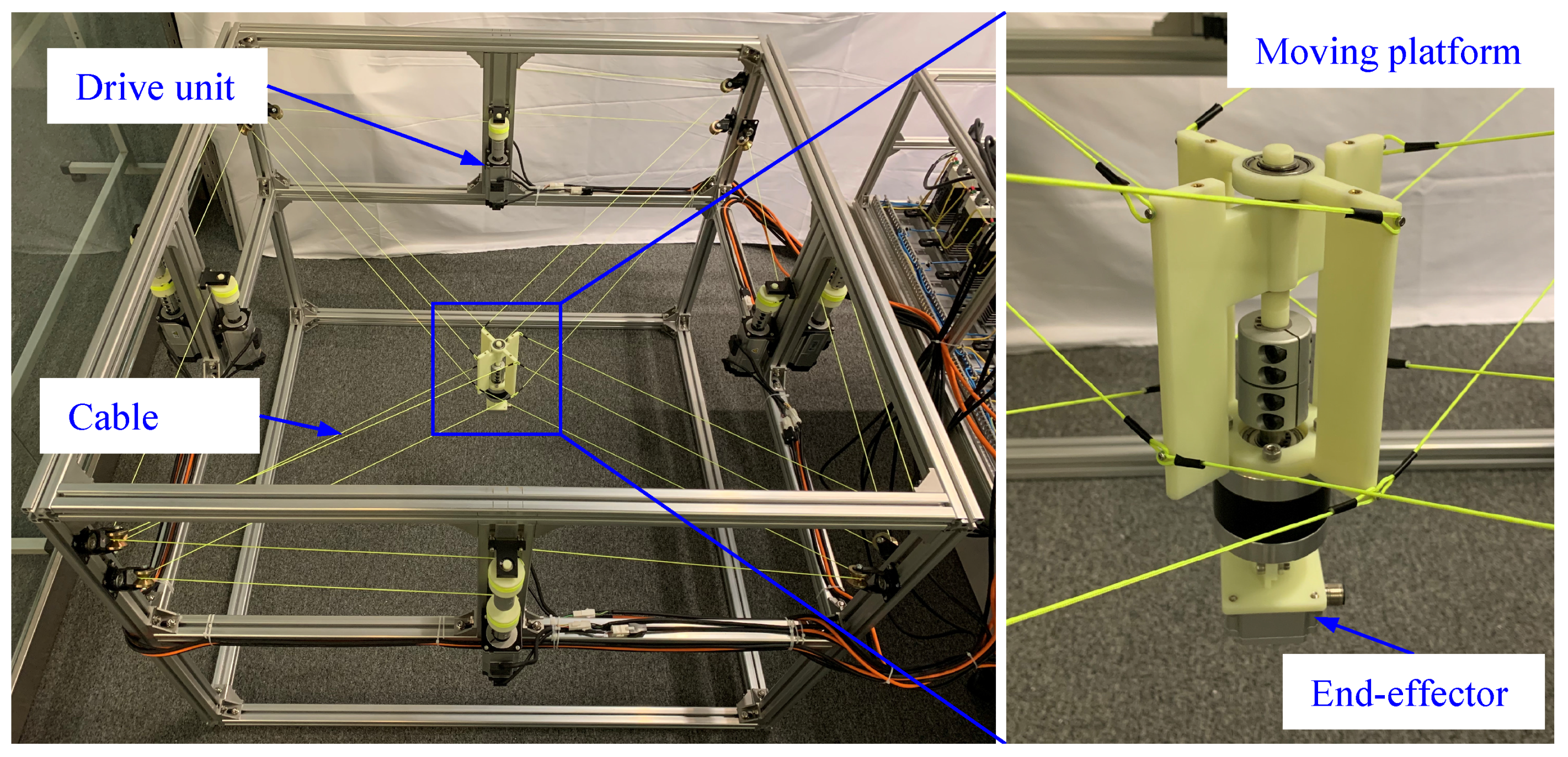
2. Architecture Description

The robot studied in this paper is a novel suspended CDPR which generates Schönflies motions. A prototype of the robot is shown in Figure 1. In this section, we briefly introduce the architecture of the robot and define some notations used in later sections.

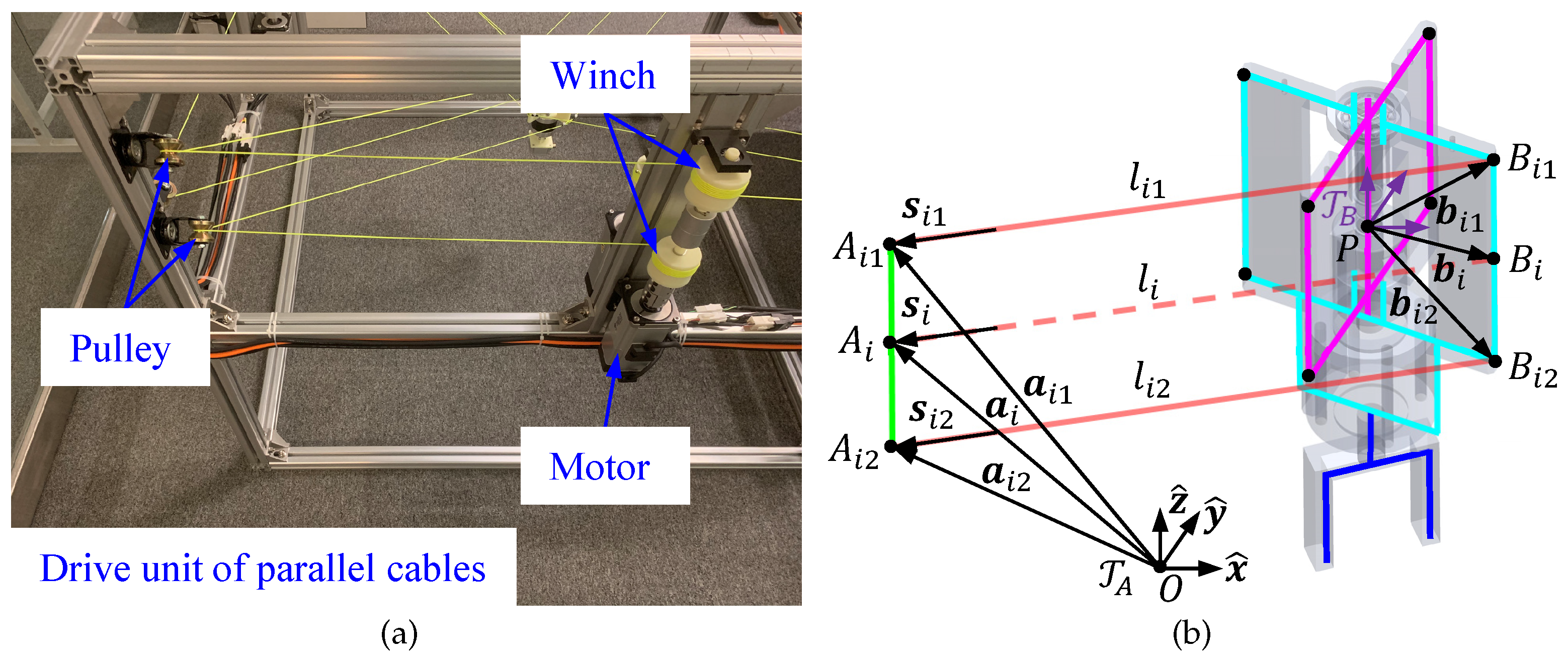
2.1. Cable Arrangement

Figure 2 shows the kinematic diagram of the novel CDPR studied in this paper. The robot has twelve driving cables linking the base and the moving platform. The cable attachment points of the robot are uniformly arranged at the vertices of the base and the moving platform. The base of the robot is cuboid-shaped, and its size is determined by three parameters: $L_{A1}$, $L_{A2}$, and $L_{A3}$. Let ${\mathcal{T}}_A$ be the inertial frame located at the geometric center point O of the base. The cable attachment points on the base are named $A_{ij}$, where $i\in \{1,2,3,4\}$ and $j\in \{1,2,3\}$. The locations from point O to points $A_{ij}$ are represented by vectors ${\mathit{a}}_{ij}$. The moving platform of the robot is composed of three parts which are articulated together. The size of the moving platform is depicted by three parameters: $L_{B1}$, $L_{B2}$, and $\Delta L_B$. Let ${\mathcal{T}}_B$ be the moving frame attached at the geometric center point P of the moving platform. The vector linking point O and point P are denoted as $\mathit{p}={\left(xyz\right)}^T$. The cable attachment points on the moving platform are named $B_{ij}$. The locations from point P to points $B_{ij}$ are represented by vectors ${\mathit{b}}_{ij}$. The cables linking points $A_{ij}$ and points $B_{ij}$ have the lengths $l_{ij}$, and their directions are represented by unit length vectors ${\mathit{s}}_{ij}$. Based on the above defined parameters, the positions of the cable attachment points of the robot are given as

$$\begin{array}{cccc}\hfill & {\mathit{a}}_{11}={\left(\begin{array}{ccc}-\frac{1}{2}{L}_{A1}& -\frac{1}{2}{L}_{A2}& \frac{1}{2}{L}_{A3}\end{array}\right)}^T,\hfill & \hfill & {\mathit{a}}_{12}={\mathit{a}}_{33}={\left(\begin{array}{ccc}-\frac{1}{2}{L}_{A1}& -\frac{1}{2}{L}_{A2}& \frac{1}{2}{L}_{A3}-L_{B2}\end{array}\right)}^T,\hfill \\ \hfill & {\mathit{a}}_{21}={\left(\begin{array}{ccc}\frac{1}{2}{L}_{A1}& -\frac{1}{2}{L}_{A2}& \frac{1}{2}{L}_{A3}\end{array}\right)}^T,\hfill & \hfill & {\mathit{a}}_{22}={\mathit{a}}_{43}={\left(\begin{array}{ccc}\frac{1}{2}{L}_{A1}& -\frac{1}{2}{L}_{A2}& \frac{1}{2}{L}_{A3}-L_{B2}+\Delta L_B\end{array}\right)}^T,\hfill \\ \hfill & {\mathit{a}}_{31}={\left(\begin{array}{ccc}\frac{1}{2}{L}_{A1}& \frac{1}{2}{L}_{A2}& \frac{1}{2}{L}_{A3}\end{array}\right)}^T,\hfill & \hfill & {\mathit{a}}_{32}={\mathit{a}}_{13}={\left(\begin{array}{ccc}\frac{1}{2}{L}_{A1}& \frac{1}{2}{L}_{A2}& \frac{1}{2}{L}_{A3}-L_{B2}\end{array}\right)}^T,\hfill \\ \hfill & {\mathit{a}}_{41}={\left(\begin{array}{ccc}-\frac{1}{2}{L}_{A1}& \frac{1}{2}{L}_{A2}& \frac{1}{2}{L}_{A3}\end{array}\right)}^T,\hfill & \hfill & {\mathit{a}}_{42}={\mathit{a}}_{23}={\left(\begin{array}{ccc}-\frac{1}{2}{L}_{A1}& \frac{1}{2}{L}_{A2}& \frac{1}{2}{L}_{A3}-L_{B2}+\Delta L_B\end{array}\right)}^T,\hfill \end{array}$$

(1)

$$\begin{array}{cccc}\hfill & {}^0{\mathit{b}}_{11}={\left(\begin{array}{ccc}\frac{1}{2}{L}_{B1}& 0& \frac{1}{2}{L}_{B2}\end{array}\right)}^T,\hfill & \hfill & {}^0{\mathit{b}}_{12}={}^0{\mathit{b}}_{13}={\left(\begin{array}{ccc}\frac{1}{2}{L}_{B1}& 0& -\frac{1}{2}{L}_{B2}\end{array}\right)}^T,\hfill \\ \hfill & {}^0{\mathit{b}}_{21}={\left(\begin{array}{ccc}\frac{1}{2}{L}_{B1}& 0& \frac{1}{2}{L}_{B2}\end{array}\right)}^T,\hfill & \hfill & {}^0{\mathit{b}}_{22}={}^0{\mathit{b}}_{23}={\left(\begin{array}{ccc}\frac{1}{2}{L}_{B1}& 0& -\frac{1}{2}{L}_{B2}+\Delta L_B\end{array}\right)}^T,\hfill \\ \hfill & {}^0{\mathit{b}}_{31}={\left(\begin{array}{ccc}-\frac{1}{2}{L}_{B1}& 0& \frac{1}{2}{L}_{B2}\end{array}\right)}^T,\hfill & \hfill & {}^0{\mathit{b}}_{32}={}^0{\mathit{b}}_{33}={\left(\begin{array}{ccc}-\frac{1}{2}{L}_{B1}& 0& -\frac{1}{2}{L}_{B2}\end{array}\right)}^T,\hfill \\ \hfill & {}^0{\mathit{b}}_{41}={\left(\begin{array}{ccc}-\frac{1}{2}{L}_{B1}& 0& \frac{1}{2}{L}_{B2}\end{array}\right)}^T,\hfill & \hfill & {}^0{\mathit{b}}_{42}={}^0{\mathit{b}}_{43}={\left(\begin{array}{ccc}-\frac{1}{2}{L}_{B1}& 0& -\frac{1}{2}{L}_{B2}+\Delta L_B\end{array}\right)}^T,\hfill \end{array}$$

(2)

$${\mathit{b}}_{ij}=\left\{\begin{array}{cc}{\mathit{R}}_z\left({\theta }_1\right){}^0{\mathit{b}}_{ij}\hfill & i\in \{1,3\},j\in \{1,2,3\}\hfill \\ {\mathit{R}}_z\left({\theta }_2\right){}^0{\mathit{b}}_{ij}\hfill & i\in \{2,4\},j\in \{1,2,3\}\hfill \end{array}\right.,$$

(3)

where ${\mathit{R}}_z(·)$ denotes the rotation matrix about the z axis, and ${\theta }_1$ and ${\theta }_2$ are two angles representing the orientation of the moving platform. The detailed definitions of ${\theta }_1$ and ${\theta }_2$ will be given in Section 2.2.

The twelve driving cables of the robot consist of four pairs of parallel cables (red lines in Figure 2) and four independent cables (yellow lines in Figure 2). During the modeling process, we use $j\in \{1,2\}$ to represent the parallel cables and use $j\in \left\{3\right\}$ to indicate the independent cables. The working principle of the parallel cables is demonstrated in Figure 3. Each pair of parallel cables is driven by two identical winches which are connected in a series and directly coupled to the same motor. The parallel cables are then passed through two identical guiding pulleys and connected to the moving platform. The arrangement of the winches and the pulleys ensures that the two cables are parallel, so they always have the same length. Based on Equations (1) and (2), we have $\left|\right|A_{i1}{A}_{i2}\left|\right|=\left|\right|B_{i1}{B}_{i2}\left|\right|$ and $A_{i1}{A}_{i2}//B_{i1}{B}_{i2}$, and thus the quadrilateral $A_{i1}{A}_{i2}{B}_{i2}{B}_{i1}$ forms a parallelogram. According to the proprieties of the parallelogram, we define $l_i=l_{i1}=l_{i2}$ and ${\mathit{s}}_i={\mathit{s}}_{i1}={\mathit{s}}_{i2}$. The parallel cables are used to constrain the rotational motion of the moving platform. When a pair of parallel cables are in tension, the moving platform cannot rotate about the normal direction of the parallelogram formed by the parallel cables. The four pairs of parallel cables are specially arranged so that the moving platform of the robot can only rotate about the vertical axis. Thus, the robot is ensured to perform Schönflies motions.

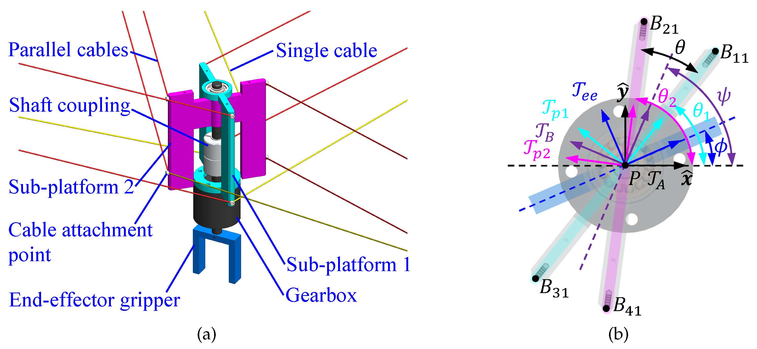
2.2. Articulated Moving Platform

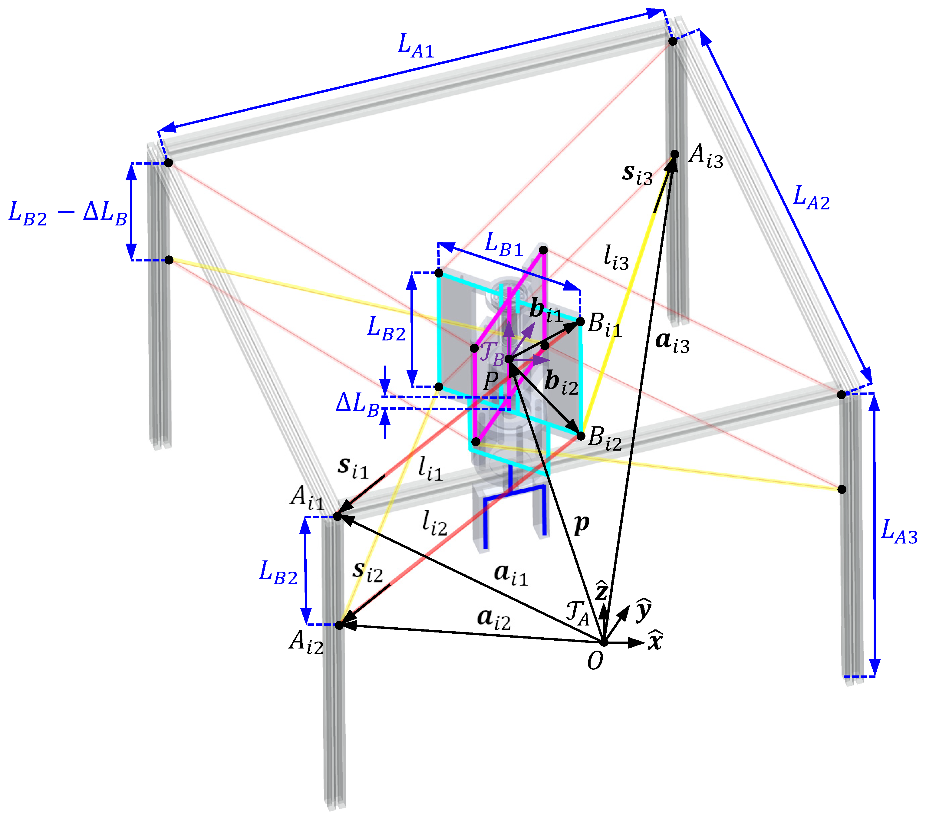
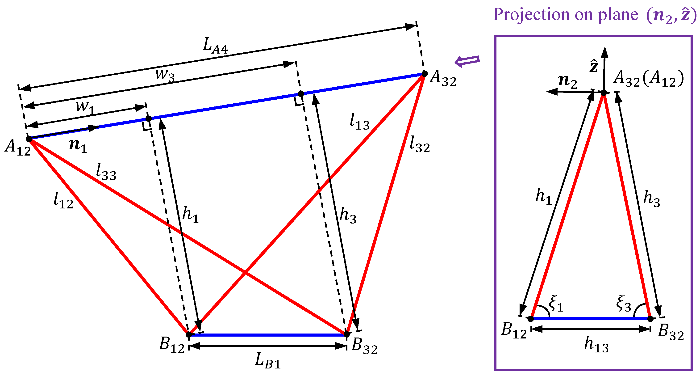
The moving platform of the robot is specially designed to extend the rotational capability of the robot about the vertical axis. Figure 4 shows the detailed architecture of the moving platform. The moving platform of the robot consists of two sub-platforms and one end-effector. The two sub-platforms are articulated together and coupled to the end-effector through a gearbox. The gearbox amplifies the relative motions between the two sub-platforms, thus extending the rotational capability of the end-effector. The two sub-platforms are named sub-platform 1 and sub-platform 2, respectively. Sub-platform 1 is shown in cyan color, and the cable attachment points on sub-platform 1 are indicated by $i\in \{1,3\}$. Sub-platform 2 is shown in the magenta color, and the cable attachment points on sub-platform 2 are indicated by $i\in \{2,4\}$. To describe the orientation of the moving platform, we attached a moving frame on each part of the moving platform at point P. Sub-platform 1 is attached with frame ${\mathcal{T}}_{p1}$, and the orientation of frame ${\mathcal{T}}_{p1}$ with respect to frame ${\mathcal{T}}_A$ is denoted as ${\theta }_1$. Sub-platform 2 is attached with frame ${\mathcal{T}}_{p2}$, and the orientation of frame ${\mathcal{T}}_{p2}$ with respect to frame ${\mathcal{T}}_A$ is denoted as ${\theta }_2$. Let $\theta$ represent the angle between the two sub-platforms, and assume the x axis of frame ${\mathcal{T}}_B$ locates on the bisectrix of $\theta$. The orientation of frame ${\mathcal{T}}_B$ with respect to frame ${\mathcal{T}}_A$ is denoted as $\psi$. Frame ${\mathcal{T}}_{ee}$ is attached on the end-effector of the robot, and the orientation of frame ${\mathcal{T}}_{ee}$ with respect to frame ${\mathcal{T}}_A$ is denoted as $\varphi$. The articulated structure of the moving platform introduces one internal DOF into the robot. We define $\psi$ and $\theta$ as the configuration of the moving platform. Then, the relations between ${\theta }_1$, ${\theta }_2$, $\varphi$ and $\psi$, $\theta$ are given as

$${\theta }_1=\psi -\frac{1}{2}\theta ,$$

(4)

$${\theta }_2=\psi +\frac{1}{2}\theta ,$$

(5)

$$\varphi =\psi +(\eta -\frac{1}{2})\theta +({\varphi }_0-{\theta }_{10})-\eta ({\theta }_{20}-{\theta }_{10}),$$

(6)

where ${\theta }_{10}$, ${\theta }_{20}$, ${\varphi }_0$ are the initial values of ${\theta }_1$, ${\theta }_2$, $\varphi$, and $\eta$ represents the amplification ratio of the gearbox.

3. Kinematics

For CDPRs, the mass and elasticity of the cables introduce a coupling relation between the kinematics and the cable tensions. Some researchers have presented approaches such as the kinetostatic modeling [23] and kinetics modeling [24] to consider these effects. However, these approaches are usually complicated and require numerical methods to solve the models. In this paper, in order to derive closed-form solutions for the kinematics of the novel CDPR, we assume the decoupling of the kinematics and the cable tensions by considering the cables as massless and inelastic straight lines. In this section, we present the kinematic modeling of the novel CDPR. Firstly, the inverse and forward kinematic problems of the robot are solved. Then, the Jacobian matrix of the robot is derived.

3.1. Inverse and Forward Kinematics

The inverse kinematic problem is to calculate the lengths of the driving cables according to the prescribed pose of the moving platform. The forward kinematic problem is to compute the pose of the moving platform according to the prescribed cable lengths. Based on the notations defined in Section 2, the pose of the moving platform in task space is defined by the generalized coordinate $\mathcal{X}$ as

$$\mathcal{X}={\left(\begin{array}{ccc}{\mathit{p}}^T& \psi {\widehat{\mathit{z}}}^T& \theta \end{array}\right)}^T={\left(\begin{array}{ccccccc}x& y& z& 0& 0& \psi & \theta \end{array}\right)}^T,$$

(7)

where $\widehat{\mathit{z}}={\left(001\right)}^T$ represents the unit length vector along the z axis. The vector of the cable lengths is given as

$$\mathit{l}={\left(\begin{array}{cccccccc}{l}_1& l_2& l_3& l_4& l_{13}& l_{23}& l_{33}& l_{43}\end{array}\right)}^T.$$

(8)

For CDPRs, the inverse kinematic problem is straightforward and generally has closed-form solutions. According to the vector loops in Figure 2, the inverse kinematic equation for the robot is derived as

$$l_{ij}=\left|\right|{\mathit{a}}_{ij}-{\mathit{b}}_{ij}-\mathit{p}\left|\right|,i\in \{1,2,3,4\},j\in \{1,2,3\}.$$

(9)

The forward kinematic problem of CDPRs is generally more involved than the inverse kinematics as there may exist multiple solutions. Numerical methods are usually adopted to solve the forward kinematics of CDPRs. By exploiting the special architecture of the robot, here we propose a geometrical approach to derive a closed-form solution for the forward kinematics of the robot. Figure 5 shows the kinematic diagram of sub-platform 1 used for the forward kinematics. Defining $L_{A4}$ as the distance between point $A_{12}$ and point $A_{32}$, we have

$$L_{A4}=\sqrt{L_{A1}^2+L_{A2}^2}.$$

(10)

For triangle $A_{12}{A}_{32}{B}_{12}$, we define $h_1$ as the altitude from vertex $B_{12}$ to side $A_{12}{A}_{32}$, and define $w_1$ as the distance between vertex $A_{12}$ and the foot of altitude $h_1$ on side $A_{12}{A}_{32}$. Since the lengths of the cables are all known, we have

$$w_1=\frac{l_{12}^2+L_{A4}^2-l_{13}^2}{2L_{A4}},$$

(11)

$$h_1=\sqrt{l_{12}^2-w_1^2}.$$

(12)

Similarly, for triangle $A_{12}{A}_{32}{B}_{32}$, we define $h_3$ as the altitude from vertex $B_{32}$ to side $A_{12}{A}_{32}$, and define $w_3$ as the distance between vertex $A_{12}$ and the foot of altitude $h_3$ on side $A_{12}{A}_{32}$. Then, $w_3$ and $h_3$ are expressed as

$$w_3=\frac{l_{33}^2+L_{A4}^2-l_{32}^2}{2L_{A4}},$$

(13)

$$h_3=\sqrt{l_{33}^2-w_3^2}.$$

(14)

Since the robot performs Schönflies motions, line $B_{12}{B}_{32}$ is always parallel with the plane formed by vectors ${\mathit{n}}_1$ and ${\mathit{n}}_2$, where ${\mathit{n}}_1$ and ${\mathit{n}}_2$ are defined as

$${\mathit{n}}_1=\frac{{\mathit{a}}_{32}-{\mathit{a}}_{12}}{\left|\right|{\mathit{a}}_{32}-{\mathit{a}}_{12}\left|\right|},$$

(15)

$${\mathit{n}}_2={\mathit{n}}_1\times \widehat{\mathit{z}}.$$

(16)

To solve the positions of points $B_{12}$ and $B_{32}$, we project the kinematic diagram onto the plane formed by vectors ${\mathit{n}}_2$ and $\widehat{\mathit{z}}$, as shown in Figure 5. The kinematic diagram becomes a triangle on the projection plane. Defining $h_{13}$ as the length of line $B_{12}{B}_{32}$ on the projection plane, we have

$$h_{13}=\sqrt{L_{B1}^2-{(w_1-w_3)}^2}.$$

(17)

Then, the two internal angles ${\xi }_1$ and ${\xi }_3$ of the triangle $A_{32}{B}_{12}{B}_{32}$ on the projection plane are derived as

$${\xi }_1=\arccos \frac{h_1^2+h_{13}^2-h_3^2}{2h_1{h}_{13}},$$

(18)

$${\xi }_3=\arccos \frac{h_3^2+h_{13}^2-h_1^2}{2h_3{h}_{13}}.$$

(19)

Now, we define ${\mathit{r}}_{12}=\mathit{p}+{\mathit{b}}_{12}$ and ${\mathit{r}}_{32}=\mathit{p}+{\mathit{b}}_{32}$ as the position vectors of points $B_{12}$ and $B_{32}$, respectively. According to Figure 5, ${\mathit{r}}_{12}$ and ${\mathit{r}}_{32}$ can be formulated as

$${\mathit{r}}_{12}=\pm h_1\cos {\xi }_1{\mathit{n}}_2-h_1\sin {\xi }_1\widehat{\mathit{z}}+{\mathit{a}}_{12}+w_1{\mathit{n}}_1,$$

(20)

$${\mathit{r}}_{32}=\mp h_3\cos {\xi }_3{\mathit{n}}_2-h_3\sin {\xi }_3\widehat{\mathit{z}}+{\mathit{a}}_{12}+w_3{\mathit{n}}_1.$$

(21)

Equations (20) and (21) determine two sets of positions for points $B_{12}$ and $B_{32}$ which are symmetrical about the plane formed by vectors ${\mathit{n}}_1$ and $\widehat{\mathit{z}}$. After obtaining the positions of point $B_{12}$ and point $B_{32}$, the position and orientation of sub-platform 1 can be derived as

$$\mathit{p}=\frac{1}{2}({\mathit{r}}_{12}+{\mathit{r}}_{32})+\frac{1}{2}{L}_{B2}\widehat{\mathit{z}},$$

(22)

$${\theta }_1=\arctan \frac{({\mathit{r}}_{12}-{\mathit{r}}_{32})·\widehat{\mathit{y}}}{({\mathit{r}}_{12}-{\mathit{r}}_{32})·\widehat{\mathit{x}}},$$

(23)

where $\widehat{\mathit{x}}={\left(100\right)}^T$ and $\widehat{\mathit{y}}={\left(010\right)}^T$. Equations (22) and (23) also determine two sets of poses of sub-platform 1. In order to determine the pose of the entire moving platform, we use the same procedure to solve the poses of sub-platform 2. Since sub-platform 1 and sub-platform 2 are articulated together, we can take the intersection of the position vectors determined by sub-platform 1 and sub-platform 2 as the true position vector of the moving platform. Then, the orientation of the moving platform can be obtained by computing Equations (4) and (5).

3.2. Jacobian Matrix

The Jacobian matrix plays an important role in the modeling and analysis of the robot as the Jacobian matrix maps the velocity of the moving platform to the velocity of the driving cables. Differentiating $\mathcal{X}$ and $\mathbf{l}$ with respect to time, we have the generalized velocity $\dot{\mathcal{X}}$ and the cable velocity $\dot{\mathit{l}}$ as

$$\dot{\mathcal{X}}={\left(\begin{array}{ccc}{\dot{\mathit{p}}}^T& \dot{\psi }{\widehat{\mathit{z}}}^T& \dot{\theta }\end{array}\right)}^T={\left(\begin{array}{ccccccc}\dot{x}& \dot{y}& \dot{z}& 0& 0& \dot{\psi }& \dot{\theta }\end{array}\right)}^T,$$

(24)

$$\dot{\mathit{l}}={\left(\begin{array}{cccccccc}{\dot{l}}_1& {\dot{l}}_2& {\dot{l}}_3& {\dot{l}}_4& {\dot{l}}_{13}& {\dot{l}}_{23}& {\dot{l}}_{33}& {\dot{l}}_{43}\end{array}\right)}^T.$$

(25)

Define ${\mathcal{V}}_{p1}$ and ${\mathcal{V}}_{p2}$ as the twist vectors of sub-platform 1 and sub-platform 2, respectively, and ${\mathcal{V}}_{ee}$ as the twist vector of the end-effector. Based on Equations (4)–(6), we have

$${\mathcal{V}}_{p1}=\left(\begin{array}{c}\dot{\mathit{p}}\\ {\dot{\theta }}_1\widehat{\mathit{z}}\end{array}\right)=\left(\begin{array}{c}\dot{\mathit{p}}\\ \dot{\psi }\widehat{\mathit{z}}-\frac{1}{2}\dot{\theta }\widehat{\mathit{z}}\end{array}\right)=\underset{{\mathit{H}}_{p1}}{\underbrace{\left[\begin{array}{cc}{\mathit{E}}_{6\times 6}& \begin{array}{c}{\mathbf{0}}_{3\times 1}\\ -\frac{1}{2}\widehat{\mathit{z}}\end{array}\end{array}\right]}}\dot{\mathcal{X}},$$

(26)

$${\mathcal{V}}_{p2}=\left(\begin{array}{c}\dot{\mathit{p}}\\ {\dot{\theta }}_2\widehat{\mathit{z}}\end{array}\right)=\left(\begin{array}{c}\dot{\mathit{p}}\\ \dot{\psi }\widehat{\mathit{z}}+\frac{1}{2}\dot{\theta }\widehat{\mathit{z}}\end{array}\right)=\underset{{\mathit{H}}_{p2}}{\underbrace{\left[\begin{array}{cc}{\mathit{E}}_{6\times 6}& \begin{array}{c}{\mathbf{0}}_{3\times 1}\\ \frac{1}{2}\widehat{\mathit{z}}\end{array}\end{array}\right]}}\dot{\mathcal{X}},$$

(27)

$${\mathcal{V}}_{ee}=\left(\begin{array}{c}\dot{\mathit{p}}\\ \dot{\varphi }\widehat{\mathit{z}}\end{array}\right)=\left(\begin{array}{c}\dot{\mathit{p}}\\ \dot{\psi }\widehat{\mathit{z}}+(\eta -\frac{1}{2})\dot{\theta }\widehat{\mathit{z}}\end{array}\right)=\underset{{\mathit{H}}_{ee}}{\underbrace{\left[\begin{array}{cc}{\mathit{E}}_{6\times 6}& \begin{array}{c}{\mathbf{0}}_{3\times 1}\\ (\eta -\frac{1}{2})\widehat{\mathit{z}}\end{array}\end{array}\right]}}\dot{\mathcal{X}},$$

(28)

where ${\mathit{E}}_{n\times n}$ represents the $n\times n$ identity matrix and ${\mathbf{0}}_{n\times m}$ represents the $n\times m$ matrix of zeros. Differentiating Equation (9) with respect to time and considering the properties of parallel cables, we have

$$\underset{{\mathit{J}}_{p1}}{\underbrace{-\left[\begin{array}{cc}{\mathit{s}}_1^T& {({\mathit{b}}_1\times {\mathit{s}}_1)}^T\\ {\mathit{s}}_3^T& {({\mathit{b}}_3\times {\mathit{s}}_3)}^T\\ {\mathit{s}}_{13}^T& {({\mathit{b}}_{13}\times {\mathit{s}}_{13})}^T\\ {\mathit{s}}_{33}^T& {({\mathit{b}}_{33}\times {\mathit{s}}_{33})}^T\end{array}\right]}}{\mathcal{V}}_{p1}=\underset{{\dot{\mathit{l}}}_{p1}}{\underbrace{\left(\begin{array}{c}{\dot{l}}_1\\ {\dot{l}}_3\\ {\dot{l}}_{13}\\ {\dot{l}}_{33}\end{array}\right)}},$$

(29)

$$\underset{{\mathit{J}}_{p2}}{\underbrace{-\left[\begin{array}{cc}{\mathit{s}}_2^T& {({\mathit{b}}_2\times {\mathit{s}}_2)}^T\\ {\mathit{s}}_4^T& {({\mathit{b}}_3\times {\mathit{s}}_4)}^T\\ {\mathit{s}}_{23}^T& {({\mathit{b}}_{23}\times {\mathit{s}}_{23})}^T\\ {\mathit{s}}_{43}^T& {({\mathit{b}}_{43}\times {\mathit{s}}_{43})}^T\end{array}\right]}}{\mathcal{V}}_{p2}=\underset{{\dot{\mathit{l}}}_{p2}}{\underbrace{\left(\begin{array}{c}{\dot{l}}_2\\ {\dot{l}}_4\\ {\dot{l}}_{23}\\ {\dot{l}}_{43}\end{array}\right)}},$$

(30)

where ${\mathit{b}}_i=({\mathit{b}}_{i1}+{\mathit{b}}_{i2})/2$, $i\in \{1,2,3,4\}$. Substituting Equations (26) and (27) into Equations (29) and (30), the velocity equation of the entire moving platform is derived as

$$\left[\begin{array}{c}{\mathit{J}}_{p1}{\mathit{H}}_{p1}\\ {\mathit{J}}_{p2}{\mathit{H}}_{p2}\end{array}\right]\dot{\mathcal{X}}=\left(\begin{array}{c}{\dot{\mathit{l}}}_{p1}\\ {\dot{\mathit{l}}}_{p2}\end{array}\right).$$

(31)

Reshaping Equation (31), we have

$$\underset{\mathit{J}}{\underbrace{-\left[\begin{array}{ccc}{\mathit{s}}_1^T& {({\mathit{b}}_1\times {\mathit{s}}_1)}^T& -\frac{1}{2}{({\mathit{b}}_1\times {\mathit{s}}_1)}^T\widehat{\mathit{z}}\\ {\mathit{s}}_2^T& {({\mathit{b}}_2\times {\mathit{s}}_2)}^T& \frac{1}{2}{({\mathit{b}}_2\times {\mathit{s}}_2)}^T\widehat{\mathit{z}}\\ {\mathit{s}}_3^T& {({\mathit{b}}_3\times {\mathit{s}}_3)}^T& -\frac{1}{2}{({\mathit{b}}_3\times {\mathit{s}}_3)}^T\widehat{\mathit{z}}\\ {\mathit{s}}_4^T& {({\mathit{b}}_4\times {\mathit{s}}_4)}^T& \frac{1}{2}{({\mathit{b}}_4\times {\mathit{s}}_4)}^T\widehat{\mathit{z}}\\ {\mathit{s}}_{13}^T& {({\mathit{b}}_{13}\times {\mathit{s}}_{13})}^T& -\frac{1}{2}{({\mathit{b}}_{13}\times {\mathit{s}}_{13})}^T\widehat{\mathit{z}}\\ {\mathit{s}}_{23}^T& {({\mathit{b}}_{23}\times {\mathit{s}}_{23})}^T& \frac{1}{2}{({\mathit{b}}_{23}\times {\mathit{s}}_{23})}^T\widehat{\mathit{z}}\\ {\mathit{s}}_{33}^T& {({\mathit{b}}_{33}\times {\mathit{s}}_{33})}^T& -\frac{1}{2}{({\mathit{b}}_{33}\times {\mathit{s}}_{33})}^T\widehat{\mathit{z}}\\ {\mathit{s}}_{43}^T& {({\mathit{b}}_{43}\times {\mathit{s}}_{43})}^T& \frac{1}{2}{({\mathit{b}}_{43}\times {\mathit{s}}_{43})}^T\widehat{\mathit{z}}\end{array}\right]}}\dot{\mathcal{X}}=\dot{\mathit{l}},$$

(32)

where $\mathit{J}$ is denoted as the Jacobian matrix of the robot.

4. Dynamics

The dynamic equation of the robot describes the relation between the actuation torques and the motion of the moving platform. The dynamic model of the robot can be formulated using finite element methods such as the SPACAR software [25], which is a general tool for the dynamic analysis of flexible multi-body systems. However, the analytical dynamic model plays an important role in the analysis and control of the robot, which can facilitate the workspace determination and lay the foundation for model-based control approaches. In this paper, we assume that the cables are massless and inelastic straight lines to derive the analytical dynamic equation of the robot. In this section, we present the dynamic modeling of the robot based on the virtual power principle. Firstly, the dynamics of the moving platform is formulated. Then, the effect of the drive trains is derived.

4.1. Dynamics of Moving Platform

The dynamic equation of the moving platform can be derived based on the virtual power principle. The friction inside the articulated joints of the moving platform is neglected, because ball bearings are installed inside the joints to reduce the friction. We define $f_{ij}$ as the tension of cable $l_{ij}$, and $f_i=f_{i1}+f_{i2}$ as the total tension of parallel cables $l_{i1}$ and $l_{i2}$. Then, the vector of the cable tensions is dented as

$${\mathit{f}}_c={\left(\begin{array}{cccccccc}{f}_1& f_2& f_3& f_4& f_{13}& f_{23}& f_{33}& f_{43}\end{array}\right)}^T.$$

(33)

For sub-platform 1, let $m_{p1}$ be the total mass, ${\mathit{r}}_{p1}$ be the position vector of the center of mass, ${\mathit{I}}_{p1}$ be the rotational inertia matrix, and ${\mathbf{\omega }}_{p1}$ be the angular velocity vector. For sub-platform 2, let $m_{p2}$ be the total mass, ${\mathit{r}}_{p2}$ be the position vector of the center of mass, ${\mathit{I}}_{p2}$ be the rotational inertia matrix, and ${\mathbf{\omega }}_{p2}$ be the angular velocity vector. Similarly, for the end-effector, let $m_{ee}$ be the total mass, ${\mathit{r}}_{ee}$ be the position vector of the center of mass, ${\mathit{I}}_{ee}$ be the rotational inertia matrix, and ${\mathbf{\omega }}_{ee}$ be the angular velocity vector. According to the virtual power principle [26], we have the dynamic equation of the moving platform as

$$\begin{array}{cc}\hfill & (m_{p1}{\ddot{\mathit{r}}}_{p1}-m_{p1}\mathit{g})·\delta {\dot{\mathit{r}}}_{p1}+({\mathit{I}}_{p1}{\dot{\mathbf{\omega }}}_{p1}+{\mathbf{\omega }}_{p1}\times {\mathit{I}}_{p1}{\mathbf{\omega }}_{p1})·\delta {\mathbf{\omega }}_{p1}+\hfill \\ \hfill & (m_{p2}{\ddot{\mathit{r}}}_{p2}-m_{p2}\mathit{g})·\delta {\dot{\mathit{r}}}_{p2}+({\mathit{I}}_{p2}{\dot{\mathbf{\omega }}}_{p2}+{\mathbf{\omega }}_{p2}\times {\mathit{I}}_{p2}{\mathbf{\omega }}_{p2})·\delta {\mathbf{\omega }}_{p2}+\hfill \\ \hfill & (m_{ee}{\ddot{\mathit{r}}}_{ee}-m_{ee}\mathit{g})·\delta {\dot{\mathit{r}}}_{ee}+({\mathit{I}}_{ee}{\dot{\mathbf{\omega }}}_{ee}+{\mathbf{\omega }}_{ee}\times {\mathit{I}}_{ee}{\mathbf{\omega }}_{ee})·\delta {\mathbf{\omega }}_{ee}={\mathit{f}}_c·\delta \dot{\mathit{l}},\hfill \end{array}$$

(34)

where $\mathit{g}={(00-9.81)}^T$ is the vector of gravitational acceleration. To formulate the dynamic equation as a function of the generalized coordinate $\mathcal{X}$, we need to derive the detailed expression of each component in Equation (34). For sub-platform 1, we define ${\mathit{c}}_{p1}$ as the position vector of the center of mass in frame ${\mathcal{T}}_{p1}$, and ${\mathit{I}}_{c1}$ as the rotational inertia matrix about the center of mass in frame ${\mathcal{T}}_{p1}$; then, we have

$${\mathit{r}}_{p1}=\mathit{p}+{\mathit{R}}_z\left({\theta }_1\right){\mathit{c}}_{p1},$$

(35)

$${\mathit{I}}_{p1}={\mathit{R}}_z\left({\theta }_1\right){\mathit{I}}_{c1}{\mathit{R}}_z{\left({\theta }_1\right)}^T.$$

(36)

Differentiating Equation (35) with respect to time, the velocity and acceleration of sub-platform 1 are expressed as

$$\begin{array}{cc}\hfill {\dot{\mathit{r}}}_{p1}& =\dot{\mathit{p}}+{\dot{\theta }}_1\widehat{\mathit{z}}\times {\mathit{R}}_z\left({\theta }_1\right){\mathit{c}}_{p1}\hfill \\ \hfill & =\underset{{\mathit{H}}_{c1}}{\underbrace{\left[\begin{array}{ccc}{\mathit{E}}_{3\times 3}& -{\left[{\mathit{R}}_z\left({\theta }_1\right){\mathit{c}}_{p1}\right]}_{\times }& \frac{1}{2}{\left[{\mathit{R}}_z\left({\theta }_1\right){\mathit{c}}_{p1}\right]}_{\times }\widehat{\mathit{z}}\end{array}\right]}}\dot{\mathcal{X}},\hfill \end{array}$$

(37)

$$\begin{array}{cc}\hfill {\ddot{\mathit{r}}}_{p1}& =\ddot{\mathit{p}}+{\ddot{\theta }}_1\widehat{\mathit{z}}\times {\mathit{R}}_z\left({\theta }_1\right){\mathit{c}}_{p1}+{\dot{\theta }}_1^2\widehat{\mathit{z}}\times \widehat{\mathit{z}}\times {\mathit{R}}_z\left({\theta }_1\right){\mathit{c}}_{p1}\hfill \\ \hfill & ={\mathit{H}}_{c1}\ddot{\mathcal{X}}+{\dot{\mathcal{X}}}^T{\mathit{H}}_{\theta 1}^T\underset{{\mathit{c}}_{c1}}{\underbrace{{\left[\widehat{\mathit{z}}\right]}_{\times }^2{\mathit{R}}_z\left({\theta }_1\right){\mathit{c}}_{p1}}}{\mathit{H}}_{\theta 1}\dot{\mathcal{X}},\hfill \end{array}$$

(38)

where ${[·]}_{\times }$ denotes the skew-symmetric matrix representation of a vector, and ${\mathit{H}}_{\theta 1}=\left(\begin{array}{ccccccc}0& 0& 0& 0& 0& 1& -\frac{1}{2}\end{array}\right)$. Since the robot performs Schönflies motions, the angular velocity and angular acceleration of sub-platform 1 are expressed as

$${\mathbf{\omega }}_{p1}={\dot{\theta }}_1\widehat{\mathit{z}}=\underset{{\mathit{H}}_{\omega 1}}{\underbrace{\left[\begin{array}{ccc}{\mathbf{0}}_{3\times 3}& {\mathit{E}}_{3\times 3}& -\frac{1}{2}\widehat{\mathit{z}}\end{array}\right]}}\dot{\mathcal{X}},$$

(39)

$${\dot{\mathbf{\omega }}}_{p1}={\ddot{\theta }}_1\widehat{\mathit{z}}={\mathit{H}}_{\omega 1}\ddot{\mathcal{X}}.$$

(40)

Then, for sub-platform 2, we define ${\mathit{c}}_{p2}$ as the position vector of the center of mass in frame ${\mathcal{T}}_{p2}$, and ${\mathit{I}}_{c2}$ as the rotational inertia matrix about the center of mass in frame ${\mathcal{T}}_{p2}$. Similar results can be obtained as follows:

$${\mathit{r}}_{p2}=\mathit{p}+{\mathit{R}}_z\left({\theta }_2\right){\mathit{c}}_{p2},$$

(41)

$${\dot{\mathit{r}}}_{p2}=\underset{{\mathit{H}}_{c2}}{\underbrace{\left[\begin{array}{ccc}{\mathit{E}}_{3\times 3}& -{\left[{\mathit{R}}_z\left({\theta }_2\right){\mathit{c}}_{p2}\right]}_{\times }& -\frac{1}{2}{\left[{\mathit{R}}_z\left({\theta }_2\right){\mathit{c}}_{p2}\right]}_{\times }\widehat{\mathit{z}}\end{array}\right]}}\dot{\mathcal{X}},$$

(42)

$${\ddot{\mathit{r}}}_{p2}={\mathit{H}}_{c2}\ddot{\mathcal{X}}+{\dot{\mathcal{X}}}^T{\mathit{H}}_{\theta 2}^T\underset{{\mathit{c}}_{c2}}{\underbrace{{\left[\widehat{\mathit{z}}\right]}_{\times }^2{\mathit{R}}_z\left({\theta }_2\right){\mathit{c}}_{p2}}}{\mathit{H}}_{\theta 2}\dot{\mathcal{X}},$$

(43)

$${\mathit{H}}_{\theta 2}=\left(\begin{array}{ccccccc}0& 0& 0& 0& 0& 1& \frac{1}{2}\end{array}\right),$$

(44)

$${\mathit{I}}_{p2}={\mathit{R}}_z\left({\theta }_2\right){\mathit{I}}_{c2}{\mathit{R}}_z{\left({\theta }_2\right)}^T,$$

(45)

$${\mathbf{\omega }}_{p2}=\underset{{\mathit{H}}_{\omega 2}}{\underbrace{\left[\begin{array}{ccc}{\mathbf{0}}_{3\times 3}& {\mathit{E}}_{3\times 3}& \frac{1}{2}\widehat{\mathit{z}}\end{array}\right]}}\dot{\mathcal{X}},$$

(46)

$${\dot{\mathbf{\omega }}}_{p2}={\mathit{H}}_{\omega 2}\ddot{\mathcal{X}}.$$

(47)

For the end-effector, we define ${\mathit{c}}_{ee}$ as the position vector of the center of mass in frame ${\mathcal{T}}_{ee}$, and ${\mathit{I}}_{ce}$ as the rotational inertia matrix about the center of mass in frame ${\mathcal{T}}_{ee}$. Then, we can derive the following results similar to sub-platform 1 and sub-platform 2:

$${\mathit{r}}_{ee}=\mathit{p}+{\mathit{R}}_z\left(\varphi \right){\mathit{c}}_{ee},$$

(48)

$${\dot{\mathit{r}}}_{ee}=\underset{{\mathit{H}}_{ce}}{\underbrace{\left[\begin{array}{ccc}{\mathit{E}}_{3\times 3}& -{\left[{\mathit{R}}_z\left(\varphi \right){\mathit{c}}_{ee}\right]}_{\times }& -(\eta -\frac{1}{2}){\left[{\mathit{R}}_z\left(\varphi \right){\mathit{c}}_{ee}\right]}_{\times }\widehat{\mathit{z}}\end{array}\right]}}\dot{\mathcal{X}},$$

(49)

$${\ddot{\mathit{r}}}_{ee}={\mathit{H}}_{ce}\ddot{\mathcal{X}}+{\dot{\mathcal{X}}}^T{\mathit{H}}_{\varphi }^T\underset{{\mathit{c}}_{ce}}{\underbrace{{\left[\widehat{\mathit{z}}\right]}_{\times }^2{\mathit{R}}_z\left(\varphi \right){\mathit{c}}_{ee}}}{\mathit{H}}_{\varphi }\dot{\mathcal{X}},$$

(50)

$${\mathit{H}}_{\varphi }=\left(\begin{array}{ccccccc}0& 0& 0& 0& 0& 1& \eta -\frac{1}{2}\end{array}\right),$$

(51)

$${\mathit{I}}_{ee}={\mathit{R}}_z\left(\varphi \right){\mathit{I}}_{ce}{\mathit{R}}_z{\left(\varphi \right)}^T,$$

(52)

$${\mathbf{\omega }}_{ee}=\underset{{\mathit{H}}_{\omega e}}{\underbrace{\left[\begin{array}{ccc}{\mathbf{0}}_{3\times 3}& {\mathit{E}}_{3\times 3}& (\eta -\frac{1}{2})\widehat{\mathit{z}}\end{array}\right]}}\dot{\mathcal{X}},$$

(53)

$${\dot{\mathbf{\omega }}}_{ee}={\mathit{H}}_{\omega e}\ddot{\mathcal{X}}.$$

(54)

Substituting the above equations into Equation (34), the dynamic equation of the moving platform can be formulated as a function of the generalized coordinate $\mathcal{X}$. Then, we have the final form of the dynamic equation of the moving platform as

$$\mathit{M}\left(\mathcal{X}\right)\ddot{\mathcal{X}}+{\dot{\mathcal{X}}}^T\mathit{C}\left(\mathcal{X}\right)\dot{\mathcal{X}}+\mathit{G}\left(\mathcal{X}\right)={\mathit{J}}^T{\mathit{f}}_c,$$

(55)

where

$$\begin{array}{cc}\hfill \mathit{M}\left(\mathcal{X}\right)=& m_{p1}{\mathit{H}}_{c1}^T{\mathit{H}}_{c1}+{\mathit{H}}_{\omega 1}^T{\mathit{R}}_z\left({\theta }_1\right){\mathit{I}}_{c1}{\mathit{R}}_z{\left({\theta }_1\right)}^T{\mathit{H}}_{\omega 1}+\hfill \\ \hfill & m_{p2}{\mathit{H}}_{c2}^T{\mathit{H}}_{c2}+{\mathit{H}}_{\omega 2}^T{\mathit{R}}_z\left({\theta }_2\right){\mathit{I}}_{c2}{\mathit{R}}_z{\left({\theta }_2\right)}^T{\mathit{H}}_{\omega 2}+\hfill \\ \hfill & m_{ee}{\mathit{H}}_{ce}^T{\mathit{H}}_{ce}+{\mathit{H}}_{\omega e}^T{\mathit{R}}_z\left(\varphi \right){\mathit{I}}_{ce}{\mathit{R}}_z{\left(\varphi \right)}^T{\mathit{H}}_{\omega e},\hfill \end{array}$$

(56)

$$\begin{array}{cc}\hfill \mathit{C}\left(\mathcal{X}\right)=& m_{p1}{\mathit{H}}_{\theta 1}^T{\mathit{H}}_{c1}^T{\mathit{c}}_{c1}{\mathit{H}}_{\theta 1}+{\mathit{H}}_{\theta 1}^T{\mathit{H}}_{\omega 1}^T{\left[\widehat{\mathit{z}}\right]}_{\times }{\mathit{R}}_z\left({\theta }_1\right){\mathit{I}}_{c1}{\mathit{R}}_z{\left({\theta }_1\right)}^T{\mathit{H}}_{\omega 1}+\hfill \\ \hfill & m_{p2}{\mathit{H}}_{\theta 2}^T{\mathit{H}}_{c2}^T{\mathit{c}}_{c2}{\mathit{H}}_{\theta 2}+{\mathit{H}}_{\theta 2}^T{\mathit{H}}_{\omega 2}^T{\left[\widehat{\mathit{z}}\right]}_{\times }{\mathit{R}}_z\left({\theta }_2\right){\mathit{I}}_{c2}{\mathit{R}}_z{\left({\theta }_2\right)}^T{\mathit{H}}_{\omega 2}+\hfill \\ \hfill & m_{ee}{\mathit{H}}_{\varphi }^T{\mathit{H}}_{ce}^T{\mathit{c}}_{ce}{\mathit{H}}_{\varphi }+{\mathit{H}}_{\varphi }^T{\mathit{H}}_{\omega e}^T{\left[\widehat{\mathit{z}}\right]}_{\times }{\mathit{R}}_z\left(\varphi \right){\mathit{I}}_{ce}{\mathit{R}}_z{\left(\varphi \right)}^T{\mathit{H}}_{\omega e},\hfill \end{array}$$

(57)

$$\begin{array}{c}\hfill \mathit{G}\left(\mathcal{X}\right)=-m_{p1}{\mathit{H}}_{c1}^T\mathit{g}-m_{p2}{\mathit{H}}_{c2}^T\mathit{g}-m_{ee}{\mathit{H}}_{ce}^T\mathit{g}.\end{array}$$

(58)

4.2. Dynamics of Drive Train

The drive unit of the robot contains a servo motor as the actuator and a winch which is directly coupled to the servo motor to drive the cable. For all the drive units of the robot, we define ${\mathbf{\tau }}_m$ as the vector of the motor torques, ${\mathbf{\theta }}_m$ as the vector of the motor rotation angles, ${\mathbf{\tau }}_f$ as the vector of the frictional torques, ${\mathit{I}}_m$ as the diagonal matrix of the moments of inertia of the winches, and $r_w$ as the radius of the winches. Based on Newton’s second law, we have

$${\mathbf{\tau }}_m+{\mathbf{\tau }}_f+r_w{\mathit{f}}_c={\mathit{I}}_m{\ddot{\mathbf{\theta }}}_m.$$

(59)

We use the Coulomb and viscous model [27] to formulate the frictional torques, and note that $r_w{\dot{\mathbf{\theta }}}_m=\dot{\mathit{l}}$. Then, the dynamic equation of the drive units of the robot is derived as

$${\mathbf{\tau }}_m=\frac{{\mathit{I}}_m}{r_w}\ddot{\mathit{l}}+{\mathit{K}}_c\mathrm{sign}\left(\frac{\dot{\mathit{l}}}{r_w}\right)+\frac{{\mathit{K}}_v}{r_w}\dot{\mathit{l}}-r_w{\mathit{f}}_c,$$

(60)

where ${\mathit{K}}_c$ represents the diagonal matrix of the Coulomb friction coefficients, and ${\mathit{K}}_v$ represents the diagonal matrix of the viscous friction coefficients.

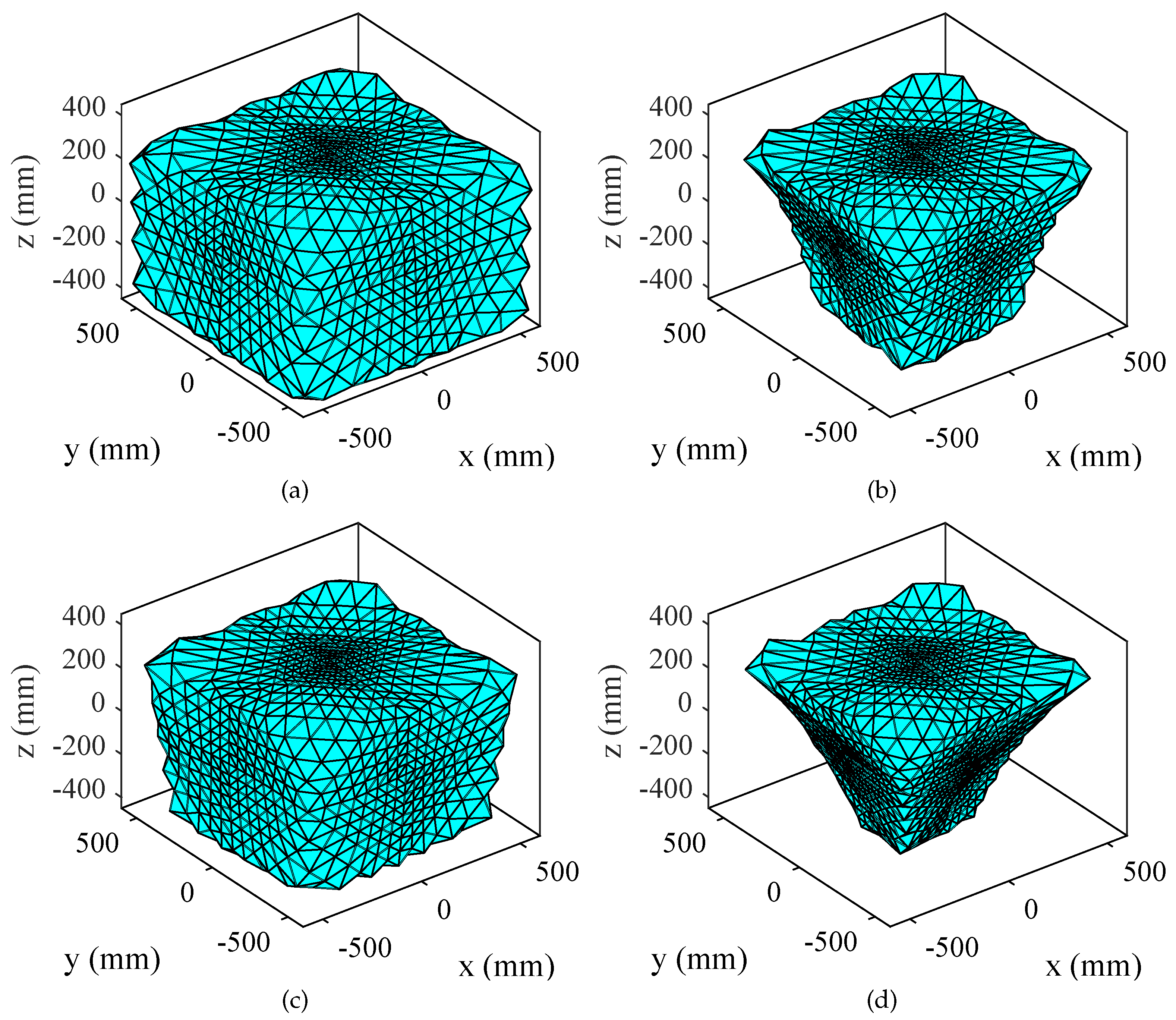
5. Workspace Analysis

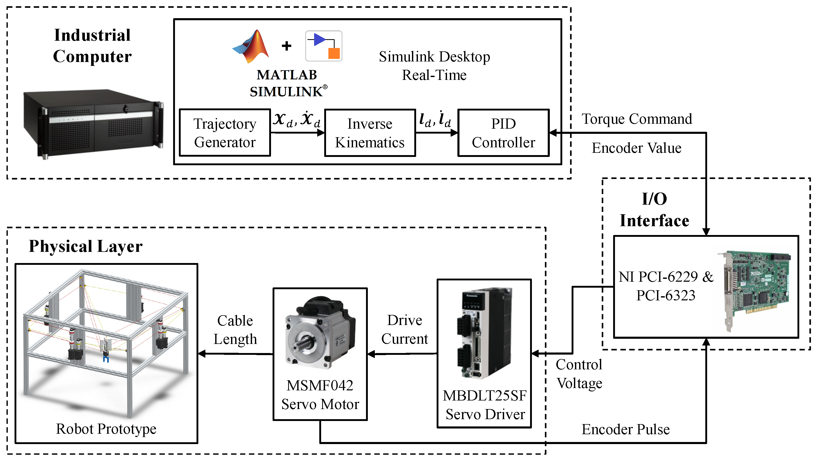
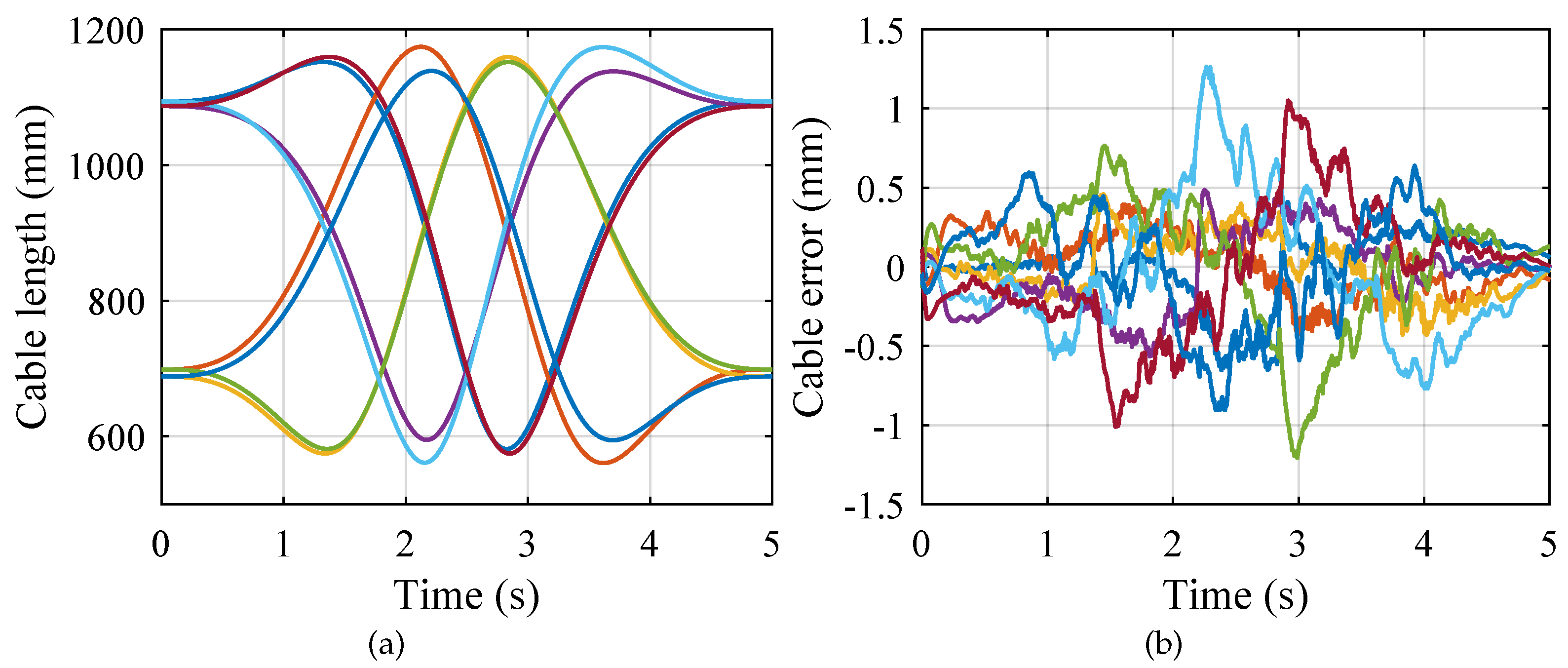
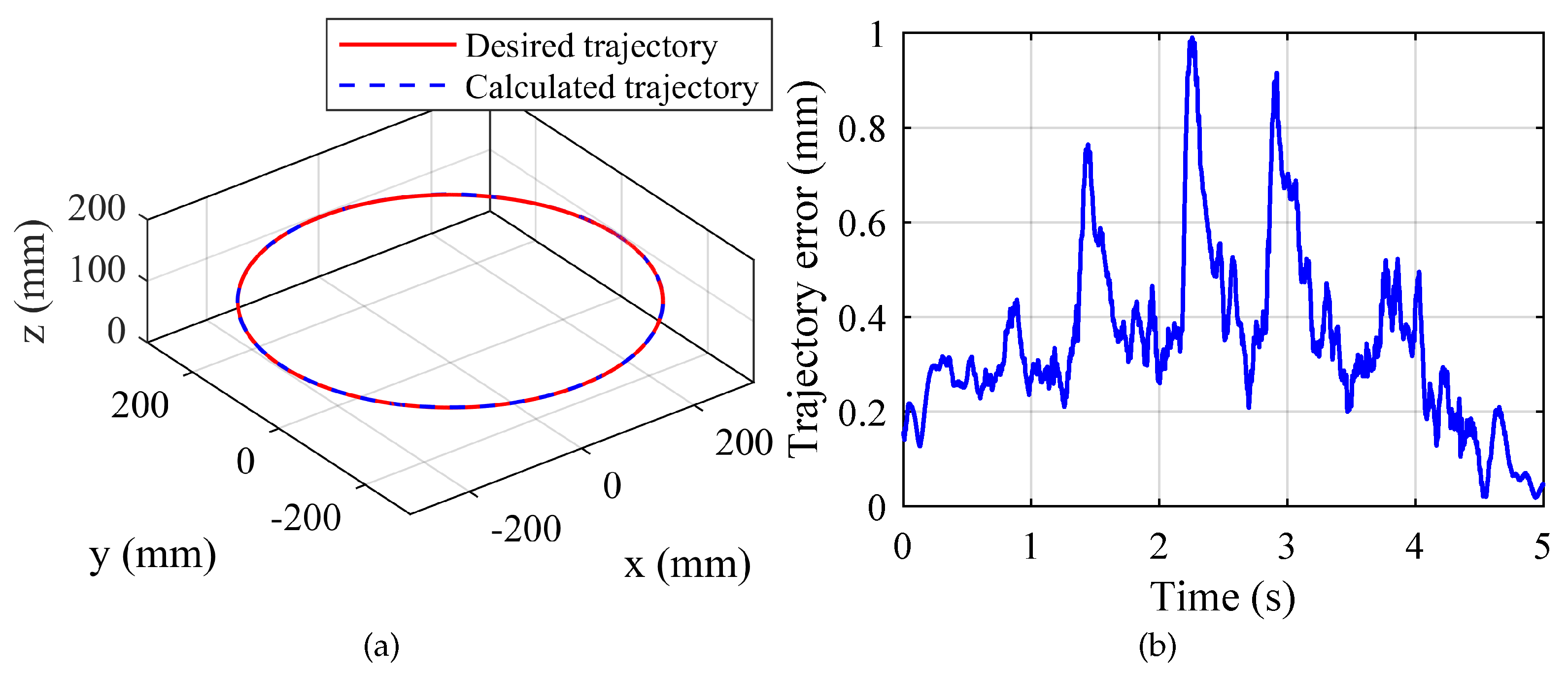
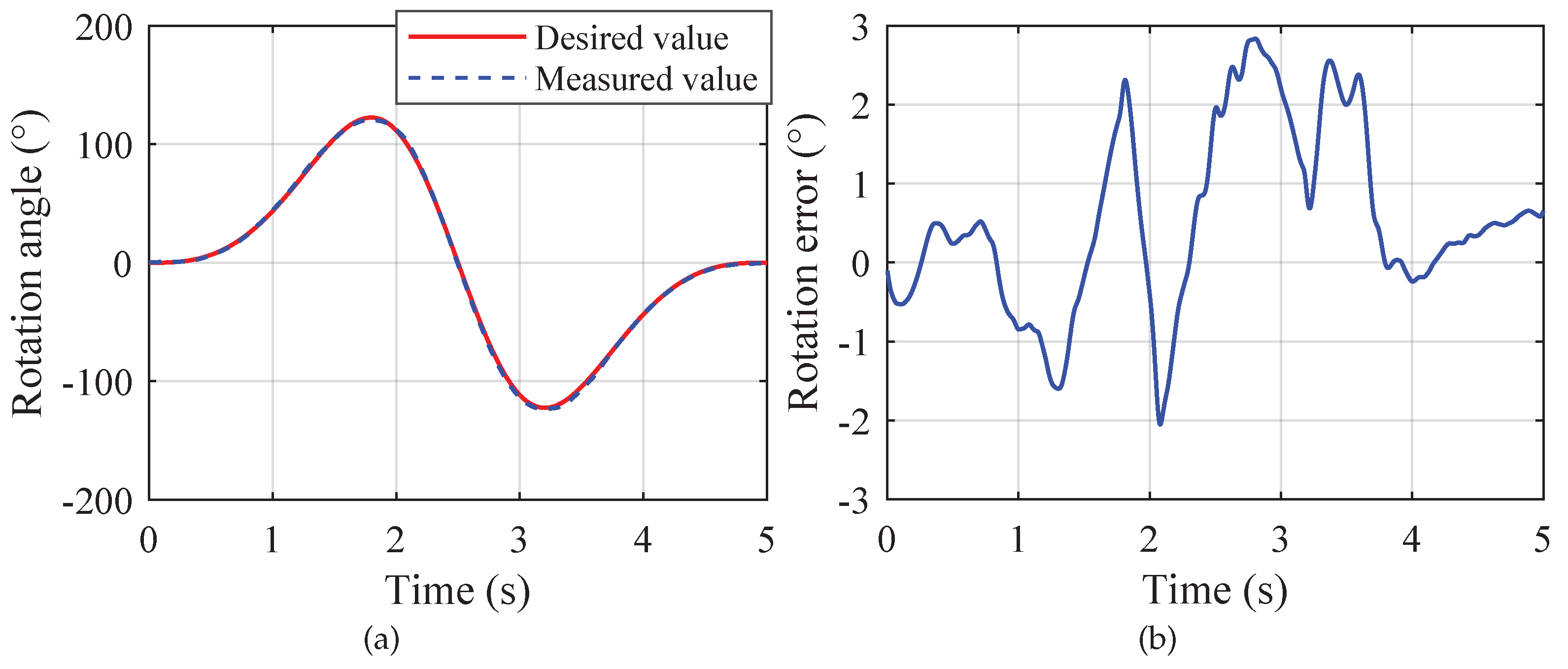
In this section, we evaluate the dynamic feasible workspace of the robot. The dynamic workspace is a set of poses where a prescribed set of moving platform accelerations can be achieved by applying feasible cable tensions. The cable tensions required for generating the prescribed accelerations can be obtained from Equation (55). For simplicity, we assume that the vectors ${\mathit{c}}_{p1}$, ${\mathit{c}}_{p2}$, and ${\mathit{c}}_{ee}$ are all parallel with the z axis of frame ${\mathcal{T}}_A$; we then have $\mathit{C}\left(\mathcal{X}\right)=\mathbf{0}$. Defining $\ddot{\mathcal{X}}={\left({\ddot{\mathit{p}}}^{T}00{\ddot{\mathbf{\alpha }}}^T\right)}^T$, $\ddot{\mathit{p}}={\left(\ddot{x}\ddot{y}\ddot{z}\right)}^T$, and $\ddot{\mathbf{\alpha }}={\left(\ddot{\psi }\ddot{\theta }\right)}^T$, the set of the required moving platform accelerations is formulated as

$${\left[\ddot{\mathcal{X}}\right]}_r=\left\{\ddot{\mathcal{X}}|{\ddot{\mathit{p}}}_{\min }⪯\ddot{\mathit{p}}⪯{\ddot{\mathit{p}}}_{\max },{\ddot{\mathbf{\alpha }}}_{\min }⪯\ddot{\mathbf{\alpha }}⪯{\ddot{\mathbf{\alpha }}}_{\max }\right\},$$

(61)

where ⪯ means the component-wise inequality. Similarly, the set of the admissible cable tensions is defined as

$${\left[{\mathit{f}}_c\right]}_a=\left\{{\mathit{f}}_c|{\mathit{f}}_{\min }⪯{\mathit{f}}_c⪯{\mathit{f}}_{\max }\right\}.$$

(62)

Thus, the dynamic feasible workspace of the robot is defined as

$${\left[\mathcal{X}\right]}_{dyn}=\left\{\mathcal{X}|\forall \ddot{\mathcal{X}}\in {\left[\ddot{\mathcal{X}}\right]}_r,\exists {\mathit{f}}_c\in {\left[{\mathit{f}}_c\right]}_a,\mathit{M}\left(\mathcal{X}\right)\ddot{\mathcal{X}}+\mathit{G}\left(\mathcal{X}\right)={\mathit{J}}^T{\mathit{f}}_c,n_c=0\right\},$$

(63)

where $n_c$ represents the number of collisions inside the robot, which is determined by calculating the distances between two cables and between the cable and the moving platform [28]. In order to investigate the effects of different acceleration values on the dynamic feasible workspace, we solve the dynamic feasible workspace of the robot in the following four scenarios:

$$\begin{array}{ccccccc}\hfill & \mathrm{Scenario}1\hfill & \hfill & {\ddot{\mathit{p}}}_{\max }=-{\ddot{\mathit{p}}}_{\min }=\left(\begin{array}{c}0\\ 0\\ 0\end{array}\right)\mathrm{mm}/{\mathrm{s}}^2,\hfill & \hfill & {\ddot{\mathbf{\alpha }}}_{\max }=-{\ddot{\mathbf{\alpha }}}_{\min }=\left(\begin{array}{c}0\\ 0\end{array}\right)\mathrm{rad}/{\mathrm{s}}^2,\hfill & \\ \hfill & \mathrm{Scenario}2\hfill & \hfill & {\ddot{\mathit{p}}}_{\max }=-{\ddot{\mathit{p}}}_{\min }=\left(\begin{array}{c}1500\\ 1500\\ 1500\end{array}\right)\mathrm{mm}/{\mathrm{s}}^2,\hfill & \hfill & {\ddot{\mathbf{\alpha }}}_{\max }=-{\ddot{\mathbf{\alpha }}}_{\min }=\left(\begin{array}{c}0\\ 0\end{array}\right)\mathrm{rad}/{\mathrm{s}}^2,\hfill & \\ \hfill & \mathrm{Scenario}3\hfill & \hfill & {\ddot{\mathit{p}}}_{\max }=-{\ddot{\mathit{p}}}_{\min }=\left(\begin{array}{c}0\\ 0\\ 0\end{array}\right)\mathrm{mm}/{\mathrm{s}}^2,\hfill & \hfill & {\ddot{\mathbf{\alpha }}}_{\max }=-{\ddot{\mathbf{\alpha }}}_{\min }=\left(\begin{array}{c}150\\ 150\end{array}\right)\mathrm{rad}/{\mathrm{s}}^2,\hfill & \\ \hfill & \mathrm{Scenario}4\hfill & \hfill & {\ddot{\mathit{p}}}_{\max }=-{\ddot{\mathit{p}}}_{\min }=\left(\begin{array}{c}1500\\ 1500\\ 1500\end{array}\right)\mathrm{mm}/{\mathrm{s}}^2,\hfill & \hfill & {\ddot{\mathbf{\alpha }}}_{\max }=-{\ddot{\mathbf{\alpha }}}_{\min }=\left(\begin{array}{c}150\\ 150\end{array}\right)\mathrm{rad}/{\mathrm{s}}^2.\hfill \end{array}$$

(64)

The kinematic and dynamic parameters of the robot are summarized in

Table 1. Kinematic and dynamic parameters of the robot.

Parameter	Notation	Value	Unit
Length of the base	$L_{A1}$	1200	$\mathrm{mm}$
Width of the base	$L_{A2}$	1200	$\mathrm{mm}$
Height of the base	$L_{A3}$	800	$\mathrm{mm}$
Length of the moving platform	$L_{B1}$	120	$\mathrm{mm}$
Height of the moving platform	$L_{B2}$	120	$\mathrm{mm}$
Offset of the moving platform height	$\Delta L_B$	$17.5$	$\mathrm{mm}$
Amplification ratio of the gearbox	$\eta$	$4.25$	-
Initial value of ${\theta }_1$	${\theta }_{10}$	$-\pi /4$	$\mathrm{rad}$
Initial value of ${\theta }_2$	${\theta }_{20}$	$\pi /4$	$\mathrm{rad}$
Initial value of $\varphi$	${\varphi }_0$	0	$\mathrm{rad}$
Mass of sub-platform 1	$m_{p1}$	$0.6$	$\mathrm{kg}$
Center of mass position of sub-platform 1	${\mathit{c}}_{p1}$	${(00-75)}^T$	$\mathrm{mm}$
Rotational inertia matrix of sub-platform 1	${\mathit{I}}_{c1}$	$\mathrm{diag}\left(1.22.54.4\right)$	$\mathrm{kg}·{\mathrm{cm}}^2$
Mass of sub-platform 2	$m_{p2}$	$0.35$	$\mathrm{kg}$
Center of mass position of sub-platform 2	${\mathit{c}}_{p2}$	${(00-75)}^T$	$\mathrm{mm}$
Rotational inertia matrix of sub-platform 2	${\mathit{I}}_{c2}$	$\mathrm{diag}\left(0.50.91.5\right)$	$\mathrm{kg}·{\mathrm{cm}}^2$
Mass of the end-effector	$m_{ee}$	$0.18$	$\mathrm{kg}$
Center of mass position of the end-effector	${\mathit{c}}_{ee}$	${(00-100)}^T$	$\mathrm{mm}$
Rotational inertia matrix of the end-effector	${\mathit{I}}_{ce}$	$\mathrm{diag}\left(0.10.10.2\right)$	$\mathrm{kg}·{\mathrm{cm}}^2$
Coulomb friction coefficient of the drive unit	$K_c$	$0.042$	-
Viscous friction coefficient of the drive unit	$K_v$	$5.3\times {10}^{-4}$	-
Upper bound of the cable tension	$f_{\max }$	50	$\mathrm{N}$
Lower bound of the cable tension	$f_{\min }$	0	$\mathrm{N}$

. To visualize the dynamic workspace of the robot in Cartesian space, the orientation of the moving platform is set as $\psi =0$ and $\theta =\pi /2$. The dynamic feasible workspace of the robot is calculated using the differential workspace hull approach [20], which approximates the hull of the workspace using a triangulation representation. Firstly, a unity sphere located at the estimated workspace center is subdivided into a set of triangular faces. Then, the boundary of the workspace is calculated along the vertices of each triangular face using a line search method. At each position, the workspace criterion is investigated for a discrete set of moving platform configurations and a Boolean result is yielded to amend the searching direction. Finally, the algorithm ends when the hull of the workspace is approximated within a certain accuracy. After determining the workspace hull, the volume of the workspace can be obtained by computing the volumes of the tetrahedrons formed by all the triangular faces.

Figure 6 shows the obtained dynamic feasible workspace in each scenario. The volume of the dynamic feasible workspace in each scenario is summarized in

Table 2. Comparison of the dynamic feasible workspace in different scenarios.

Scenario	Scenario 1	Scenario 2	Scenario 3	Scenario 4
Volume of the robot covered by the dynamic feasible workspace	$71.08\%$	$37.89\%$	$56.54\%$	$26.43\%$

. In Scenario 1, where the required acceleration set is empty, the dynamic feasible workspace is actually equivalent to the static feasible workspace. The volume of the dynamic feasible workspace in Scenario 1 is the largest among the four scenarios, and the shape of the workspace is like a cuboid similar to the base. In Scenario 2, the moving platform of the robot only needs to perform linear accelerations. The shape of the dynamic workspace in Scenario 2 is like a frustum whose cross-section increases along the z direction. The workspace volume in Scenario 2 is reduced by $46.69\%$ compared with Scenario 1. In Scenario 3 where only angular accelerations are required, the dynamic feasible workspace is reduced by $20.46\%$ compared with Scenario 1. Comparing Scenario 3 with Scenario 2, it is observed that the angular accelerations have a weaker effect on the volume of the dynamic feasible workspace. In Scenario 4, the moving platform is required to perform both linear and angular accelerations. The dynamic feasible workspace in Scenario 4 is the smallest among the four scenarios, and its volume is reduced by $62.82\%$ compared with Scenario 1. The shape of the dynamic workspace in Scenario 4 is similar to that of the workspace in Scenario 2, which indicates that the values of linear accelerations play a decisive role in determining the dynamic feasible workspace of the robot.

6. Experiment

To validate the correctness of the previously derived models and workspace, in this section, we performed experiments on the robot prototype shown in Figure 1. The main parameters of the prototype are summarized in Table 1. The control system diagram of the prototype which demonstrates the working principle and main components of the prototype system is shown in Figure 7. The control algorithms were implemented in the real-time kernel of Simulink Desktop Real-Time on an industrial computer. A proportional-integral-derivative (PID) controller was deigned in joint space with the sample rate of $1\mathrm{kHz}$ to control the prototype. At the current stage, the robot prototype was not equipped with tension sensors; the cable tensions were therefore not available in the experimental results.

In the experiments, the robot prototype was controlled to track a predefined trajectory inside the workspace. A circular trajectory located near the boundary of the dynamic feasible workspace determined in Section 5 was designed as

$$\begin{array}{ccccc}\hfill & x_d=300\cos \left(2\pi s\right)\mathrm{mm},\hfill & \hfill & {\psi }_d=10\sin \left(2\pi s\right){}^{\circ },\hfill & \\ \hfill & y_d=300\sin \left(2\pi s\right)\mathrm{mm},\hfill & \hfill & {\theta }_d=30\sin \left(2\pi s\right)+90{}^{\circ },\hfill & \\ \hfill & z_d=100\mathrm{mm},\hfill & \hfill & s=10{\left(\frac{t}{T}\right)}^3-15{\left(\frac{t}{T}\right)}^4+6{\left(\frac{t}{T}\right)}^5,\hfill \end{array}$$

(65)

where $T=5\mathrm{s}$ is the period of the trajectory. The trajectory was successfully tracked by the robot prototype and no cable slackness was observed, which demonstrates that the robot can perform dynamic trajectories with feasible cable tensions inside the dynamic feasible workspace. Figure 8 shows the trajectory tracking performance of the robot prototype in joint space. The desired cable lengths were obtained by calculating the inverse kinematics based on the robot trajectory in Equation (65). These values were fed into the robot controller as reference signals. The cable length errors were measured with the encoders on the servo motors. The maximum error among all the cables was $1.26\mathrm{mm}$, which demonstrates that the robot has a high tracking accuracy in joint space. Based on the measured cable lengths, the task space trajectory performed by the robot prototype can be obtained by calculating the forward kinematics of the robot. Figure 9 presents the comparison of the desired trajectory and the calculated trajectory from the forward kinematics in Cartesian space. The average tracking error and the maximum tracking error along the Cartesian space trajectory were $0.35\mathrm{mm}$ and $0.99\mathrm{mm}$, respectively. These results verify the consistency of the inverse and forward kinematic models of the robot derived in Section 3. However, the real trajectory performed by the robot may deviate from the calculated trajectory because the unmodeled uncertainties and the manufacturing errors were neglected. To evaluate the rotational accuracy of the robot, an LPMS-IG1 inertial measurement unit (IMU) was installed on the end-effector of the robot prototype to measure the rotation angle. Figure 10 shows the rotation angle of the end-effector along the testing trajectory. The desired value of the rotation angle was calculated using Equation (6) based on the robot trajectory, and the measured value was obtained from the IMU sensor. The rotation error of the end-effector varied from $-2.05{}^{\circ }$ to $2.81{}^{\circ }$, with an average value of $0.54{}^{\circ }$. Taking into account the manufacturing and assembly errors of the prototype, these values can be considered acceptable. The experimental results in this section validate the correctness of the previously derived models and workspace, and demonstrate the feasibility of the proposed robot in generating Schönflies motions.

7. Conclusions

In this paper, kinematic and dynamic modeling and a workspace analysis of a novel suspended CDPR for Schönflies motions were presented. The inverse and forward kinematic problems of the robot were solved through a geometrical approach. The dynamic equation of the robot was derived by separately considering the moving platform and the drive trains. Based on the dynamic equation, the dynamic feasible workspace of the robot was determined under different values of accelerations. The correctness of the derived models and the workspace was verified through experiments on a prototype of the robot. In future works, we will develop a cable tension measurement system and use a motion capture system to measure the poses of the robot for further validation of the models derived in this paper.

References

1. Gosselin, C. Cable-driven parallel mechanisms: State of the art and perspectives. Mech. Eng. Rev. 2014, 1, DSM0004. [Google Scholar] [CrossRef] [Green Version]
2. Tang, X. An overview of the development for cable-driven parallel manipulator. Adv. Mech. Eng. 2014, 6, 823028. [Google Scholar] [CrossRef] [Green Version]
3. Tempel, P.; Schnelle, F.; Pott, A.; Eberhard, P. Design and programming for cable-driven parallel robots in the German Pavilion at the EXPO 2015. Machines 2015, 3, 223–241. [Google Scholar] [CrossRef]
4. Jiang, X.; Barnett, E.; Gosselin, C. Dynamic point-to-point trajectory planning beyond the static workspace for six-DOF cable-suspended parallel robots. IEEE Trans. Robot. 2018, 34, 781–793. [Google Scholar] [CrossRef]
5. Jamshidifar, H.; Rushton, M.; Khajepour, A. A reaction-based stabilizer for nonmodel-based vibration control of cable-driven parallel robots. IEEE Trans. Robot. 2020, 37, 667–674. [Google Scholar] [CrossRef]
6. Zarebidoki, M.; Dhupia, J.S.; Xu, W. A review of cable-driven parallel robots: Typical configurations, analysis techniques, and control methods. IEEE Robot. Autom. Mag. 2022, 2–19. [Google Scholar] [CrossRef]
7. Paty, T.; Binaud, N.; Caro, S.; Segonds, S. Cable-driven parallel robot modelling considering pulley kinematics and cable elasticity. Mech. Mach. Theory 2021, 159, 104263. [Google Scholar] [CrossRef]
8. Zhang, Z.; Xie, G.; Shao, Z.; Gosselin, C. Kinematic calibration of cable-driven parallel robots considering the pulley kinematics. Mech. Mach. Theory 2022, 169, 104648. [Google Scholar] [CrossRef]
9. Mishra, U.A.; Caro, S. Forward kinematics for suspended under-actuated cable-driven parallel robots with elastic cables: A neural network approach. ASME J. Mech. Robot. 2022, 14, 041008. [Google Scholar] [CrossRef]
10. Zi, B.; Zhang, L.; Zhang, D.; Qian, S. Modeling, analysis, and co-simulation of cable parallel manipulators for multiple cranes. Proc. Inst. Mech. Eng. Part C J. Mech. Eng. Sci. 2015, 229, 1693–1707. [Google Scholar] [CrossRef]
11. Zi, B.; Sun, H.; Zhang, D. Design, analysis and control of a winding hybrid-driven cable parallel manipulator. Robot. Comput.-Integr. Manuf. 2017, 48, 196–208. [Google Scholar] [CrossRef]
12. Ferravante, V.; Riva, E.; Taghavi, M.; Braghin, F.; Bock, T. Dynamic analysis of high precision construction cable-driven parallel robots. Mech. Mach. Theory 2019, 135, 54–64. [Google Scholar] [CrossRef]
13. Wang, R.; Li, Y. Analysis and multi-objective optimal design of a planar differentially driven cable parallel robot. Robotica 2021, 39, 2193–2209. [Google Scholar] [CrossRef]
14. Abbasnejad, G.; Eden, J.; Lau, D. Generalized ray-based lattice generation and graph representation of wrench-closure workspace for arbitrary cable-driven robots. IEEE Trans. Robot. 2018, 35, 147–161. [Google Scholar] [CrossRef]
15. Gouttefarde, M.; Daney, D.; Merlet, J.P. Interval-analysis-based determination of the wrench-feasible workspace of parallel cable-driven robots. IEEE Trans. Robot. 2010, 27, 1–13. [Google Scholar] [CrossRef] [Green Version]
16. Gagliardini, L.; Gouttefarde, M.; Caro, S. Determination of a dynamic feasible workspace for cable-driven parallel robots. In Advances in Robot Kinematics; Springer: Cham, Swizterland, 2018; pp. 361–370. [Google Scholar]
17. Zhang, Z.; Shao, Z.; Wang, L. Optimization and implementation of a high-speed 3-DOFs translational cable-driven parallel robot. Mech. Mach. Theory 2020, 145, 103693. [Google Scholar] [CrossRef]
18. Zhang, Z.; Shao, Z.; Peng, F.; Li, H.; Wang, L. Workspace analysis and optimal design of a translational cable-driven parallel robot with passive springs. ASME J. Mech. Robot. 2020, 12, 051005. [Google Scholar] [CrossRef]
19. Tang, X.; Wang, W.; Tang, L. A geometrical workspace calculation method for cable-driven parallel manipulators on minimum tension condition. Adv. Robot. 2016, 30, 1061–1071. [Google Scholar] [CrossRef]
20. Pott, A. Efficient computation of the workspace boundary, its properties and derivatives for cable-driven parallel robots. In Computational Kinematics; Springer: Cham, Swizterland, 2018; pp. 190–197. [Google Scholar]
21. Wang, Y.; Belzile, B.; Angeles, J.; Li, Q. Kinematic analysis and optimum design of a novel 2PUR-2RPU parallel robot. Mech. Mach. Theory 2019, 139, 407–423. [Google Scholar] [CrossRef]
22. Meng, Q.; Liu, X.J.; Xie, F. Design and development of a Schönflies-motion parallel robot with articulated platforms and closed-loop passive limbs. Robot. Comput.-Integr. Manuf. 2022, 77, 102352. [Google Scholar] [CrossRef]
23. Gouttefarde, M.; Nguyen, D.Q.; Baradat, C. Kinetostatic analysis of cable-driven parallel robots with consideration of sagging and pulleys. In Advances in Robot Kinematics; Springer: Cham, Swizterland, 2014; pp. 213–221. [Google Scholar]
24. Hu, X.; Cao, L.; Luo, Y.; Chen, A.; Zhang, E.; Zhang, W. A novel methodology for comprehensive modeling of the kinetic behavior of steerable catheters. IEEE/ASME Trans. Mechatron. 2019, 24, 1785–1797. [Google Scholar] [CrossRef]
25. Zhang, W.; Werf, K. Automatic communication from a neutral object model of mechanism to mechanism analysis programs based on a finite element approach in a software environment for CADCAM of mechanisms. Finite Elem. Anal. Des. 1998, 28, 209–239. [Google Scholar] [CrossRef]
26. Yang, X.; Wu, H.; Li, Y.; Kang, S.; Chen, B. Computationally efficient inverse dynamics of a class of six-DOF parallel robots: Dual quaternion approach. J. Intell. Robot. Syst. 2019, 94, 101–113. [Google Scholar] [CrossRef]
27. Liu, Y.; Li, J.; Zhang, Z.; Hu, X.; Zhang, W. Experimental comparison of five friction models on the same test-bed of the micro stick-slip motion system. Mech. Sci. 2015, 6, 15–28. [Google Scholar] [CrossRef] [Green Version]
28. Nguyen, D.Q.; Gouttefarde, M. On the improvement of cable collision detection algorithms. In Cable-Driven Parallel Robots; Springer: Cham, Swizterland, 2015; pp. 29–40. [Google Scholar]
Figure 1. Prototype of the novel cable-driven parallel robot (CDPR).
Machines 10 00451 g001
Figure 2. Kinematic diagram of the novel CDPR.
Machines 10 00451 g002
Figure 3. Working principle of parallel cables. (a) Drive unit. (b) Kinematic diagram.
Machines 10 00451 g003
Figure 4. Architecture of the articulated moving platform. (a) Front view. (b) Top view.
Machines 10 00451 g004
Figure 5. Kinematic diagram of sub-platform 1 for forward kinematics.
Machines 10 00451 g005
Figure 6. Dynamic feasible workspace of the robot in different scenarios. (a) Scenario 1. (b) Scenario 2. (c) Scenario 3. (d) Scenario 4.
Machines 10 00451 g006
Figure 7. Control system diagram of the robot prototype.
Machines 10 00451 g007
Figure 8. Trajectory tracking performance in joint space. (a) Desired cable lengths. (b) Cable length errors.
Machines 10 00451 g008
Figure 9. Trajectory tracking performance in Cartesian space. (a) Desired trajectory and calculated trajectory. (b) Trajectory error.
Machines 10 00451 g009
Figure 10. Rotation angle of the end-effector. (a) Desired value and measured value. (b) Rotation error.
Machines 10 00451 g010