Towards Self-Adaptability of Instrumented Electromagnetic Energy Harvesters

Abstract

Motion-driven electromagnetic energy harvesting is a well-suited technological solution to autonomously power a broad range of autonomous devices. Although different harvester configurations and mechanisms have been already proposed to perform effective tuning and broadband harvesting, no methodology has proven to be effective to maximize the harvester performance for unknown and time-varying patterns of mechanical power sources externally exciting the harvesters. This paper provides, for the first time, a radically new concept of energy harvester to maximize the harvested energy for time-varying excitations: the self-adaptive electromagnetic energy harvester. This research work aims to analyze the electric energy harvesting gain when self-adaptive electromagnetic harvesters, using magnetic levitation architectures, are able to autonomously adapt their architecture as variations in the excitation patterns occur. This was accomplished by identifying the optimal harvester length for different excitation patterns and load resistances. Gains related to electric current and power exceeding 100 can be achieved for small-scale harvesters. The paper also describes comprehensive case studies to verify the feasibility of the self-adaptive harvester, considering the energy demand from the adaptive mechanism, namely the sensing, processing and actuation systems. These successful results highlight the potential of this innovative methodology to design highly sophisticated energy harvesters, both for a small- and large-scale power supply.

1. Introduction

The research on energy harvesting is a promising and emerging field that has been received broad interest within both the academic community and industry [1]. In the past few years, energy generation from ambient mechanical sources has emerged as a promising methodology to inexhaustibly power both large-scale and small-scale electronic device systems [2,3,4].Regarding the scope of small-scale powering, a wide range of technologies require long-term operation, reduced performance losses, low maintenance and performance adaptability to external mechanical excitations [5]. These are emerging technologies aiming to develop high-performance autonomous remote sensors, multifunctional implantable biomedical devices, wearable devices, mobile applications, IoT and communication networks, among many others, in which the self-powering ability is recognized as critical [6,7,8,9,10,11,12].

Among the great amount of energy harvesters already designed, the most relevant are based on electromagnetic, piezoelectric, electrostatic and triboelectric transduction mechanisms to convert the ubiquitous mechanical energy into electric energy [5]. This work is focused on the electromagnetic energy harvesting using magnetic levitation architectures, as they hold potential to autonomously power a wide range of technologies. This is due to their low-cost and non-complex design, low maintenance requirements, effective harvesting even for structures with severe dimensional constraints, ability to operate with stable performance for long periods of time and the ability to generate electricity as a complementary source of conventional renewable energy sources [5,6,13,14,15,16,17,18]. Moreover, both small- and large-scale real-world applications can be powered by electromagnetic harvesters using magnetic levitation architectures [6,10,11,15]. Although this is a very promising harvesting approach, its current technology state was only able to provide up to 8 mW/cm${}^3$ (8 kW/m${}^3$) and with no self-tuning capability to time-varying excitations [5,19]. This lack of effective optimization procedures has been mainly caused by: (i) the use of complex tuning mechanics, which remain not suitable for unknown, broadband and time-varying mechanical power sources, particularly when strong dimensional constraints are considered; (ii) non-detailed analyses of the influence of the design configuration, mainly concerning the distance between fixed magnets (which ensures the inertial motion of levitating magnet(s)) [6,20,21,22,23,24,25].

A self-adaptive energy harvester with the ability to automatically adapt its architecture as a function of time-varying excitation patterns has not been proposed so far. Among all the parameters prone to optimization, the harvester length (the distance between non-levitating magnets on the magnetic levitation architecture) can be easily controlled such that an optimal length can be defined for each excitation. The main goal of this study is to analyze the impact of this innovative approach using a well-known analytical model that is experimentally validated. The observed significant performance improvements in terms of electric power gains, in comparison with the non-adaptive operation, provide strong motivation and justification for further advances and applications.

2. Methods

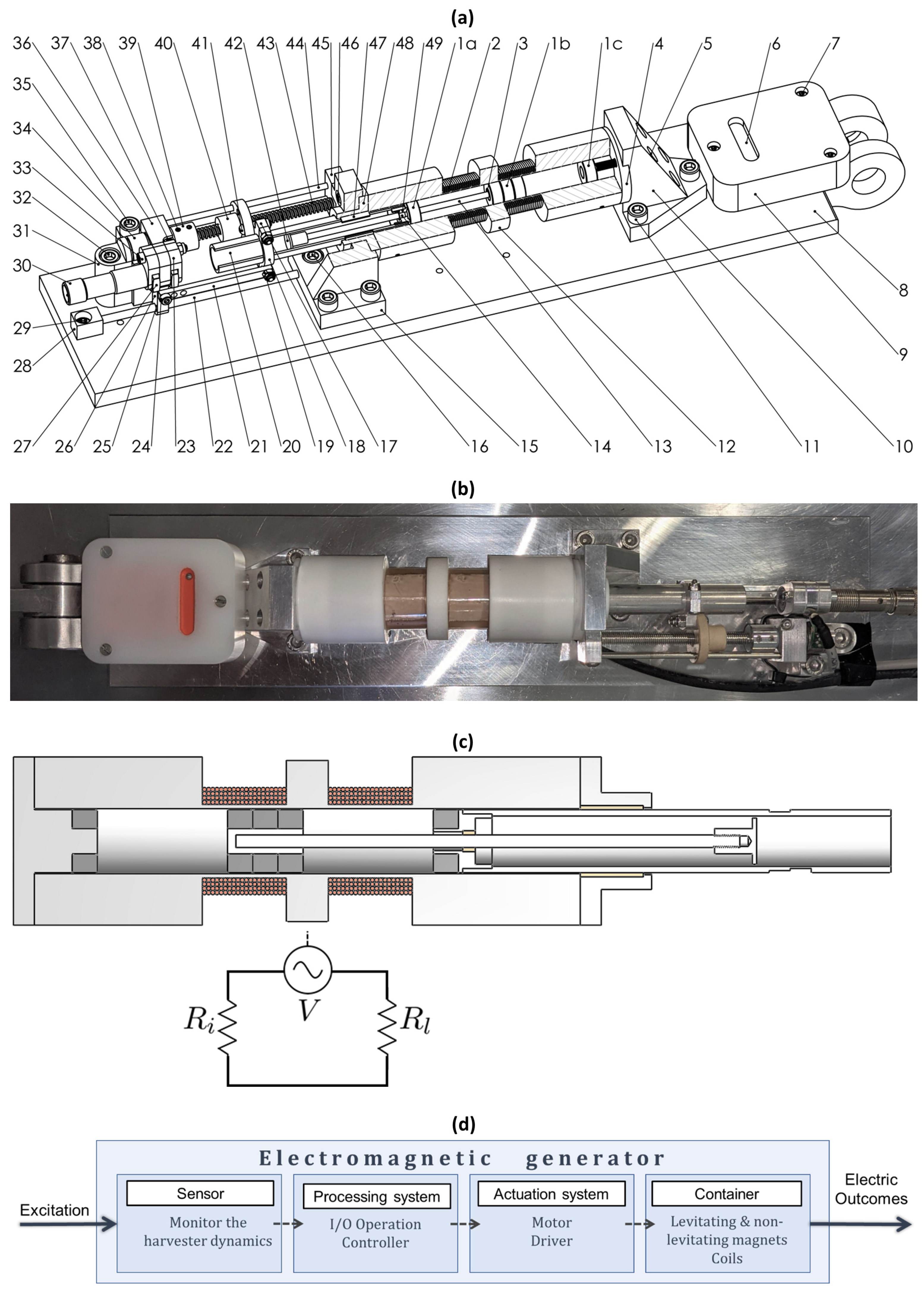
2.1. Electromagnetic Harvester Design

The architecture and schematic diagram of the motion-driven electromagnetic energy harvester considered in this study is illustrated in Figure 1a–d. As shown in Figure 1a, it is composed by a hollowed cylindrical structure (12); two multi-layered coils (2) wound around a portion of the outer housing; and five hard magnetic elements, in which two (1a, 1c) are fixed to the end extremities of the container, and three (1b) are experiencing levitation (as they are positioned between the fixed ones). This is a non-complex architecture widely reported in the literature, which includes the fundamental elements of the transduction process, and it is also suitable for analyzing innovative optimization methodologies [5,6,14,26]. Moreover, several relevant models that describe the transduction mechanism of this harvester were already developed and experimentally validated by some authors [6,14,17,18,19]. Ring magnets were used, allowing the inertial guiding rod (which is coupled to the levitating magnet) to pass through the center of the hard magnetic elements. The coils are connected in series and electrically connected to a resistive load (Figure 1c). All magnets and coils are installed concentrically to the container body (12). One of the non-levitating magnets (1c) is fixed to the harvester lid (4), while the axial positioning of the other (1a) can autonomously be self-adapted inside the container by means of an open-loop processing system and according to the dynamics of the mechanical vibrational excitations. The inertial mass consists of three permanent magnets (1b) in levitation, a guiding rod (13), magnet–rod coupling (3) and inertial mass extremity (42). To maximize the harvester performance, the container was manufactured using PTFE, as it ensures a low friction coefficient; the architecture was designed to ensure a tight-fitting container–magnet interface. Moreover, appropriate materials with negligible magnetic permeability and electrical conductivity properties were carefully selected. The sleeve bearing (14), installed inside the tube–magnet coupling (49), concentrically guides the inertial guiding rod (13), ensuring lower coefficients of mechanical friction. The section increase in the inertial mass tip at extremity (42) allows the sensor (30) to acquire the dynamics of the inertial mass. The container (12) is positioned and firmly screwed (5, 46) between two lids (4, 48), which in turn are embedded in the supports (10, 15); the entire instrumented harvester assembly is fixed with screws on the aluminium board (8). The actuation system is composed by a stepper motor (34), trapezoidal spindle screw (43), motor–spindle coupling (39), sliding nut (40), guiding shafts (44), tube (20), tube–nut fastener (17, 18), tube–magnet coupling (49), sleeve bearings (25, 47), supports (31, 36, 45), screws (32, 35, 37, 41), lock nuts (19) and studs (38). The actuation system acts on the non-levitating magnet (1a), which in turn is installed at the end of the tube–magnet coupling (49). The dynamics of the external mechanical energy source is monitored by the accelerometer (6), which is embedded in a housing (9) and fixed to the board (8) by means of screws (7). The instrumented harvester comprises a second sensing system, consisting of an ultrasonic sensor (30), respective nuts (27) and supports (26,28), anti-vibration fasteners (23), screws (24, 29, 33), lock nut (19), spacer (21), sleeve bearing (25) and shaft (22). The sensor (30) is installed concentrically with the container (12) and rigidly fixed to the tube through the spacer (21), moving with the actuation system.

The operating method of the open-loop electric linear power generator comprises the following stages: (i) predetermination the optimal position of the non-levitating magnet (1a) for different (frequency and amplitude) mechanical excitation dynamics; (ii) incorporation of these optimal positions in the internal memory of the processing system; (iii) reading of the mechanical excitation dynamics using the accelerometer (6); (iv) identification of the optimal harvester length using the information available in the internal memory of the processing system; (v) positioning of the adaptive non-levitating magnet (1a), using the actuation system and according to the reading of the accelerometer (6), as shown in Figure 1d.

2.2. Mechanical–Electric Transduction Mechanism

The repulsive (levitation) magnetic force is approached as a cubic non-linear spring, such that the harvesting system behaves as a Duffing oscillator. Therefore, the equivalent force–displacement curve is given by a summation of the restoring magnetic forces ($F_m$) acting on the bottom and top hard magnetic elements along the axial direction, according to Equation (1), where k is the linear stiffness and $k_3$ is the non-harmonic coefficient [14].

$$F_m=kx+k_3{x}^3$$

(1)

This study uses two references frames: the reference z is used to describe the dynamics of the mechanical power source externally exciting the harvester, which is defined in terms of amplitude (A) and frequency ($\mathsf{\Omega }$); and the reference x describes the dynamics of the inertial levitating magnet. The model that describes the interplay between electrical and mechanical dynamics is expressed by Equation (2) [14]:

$$\left\{\begin{array}{c}m\ddot{y}+c_m\dot{y}+ky+k_3{y}^3+\alpha I+mg={\omega }^2{A}_{z}cos\left(\omega t\right)\hfill \\ I=\frac{\alpha }{R_l+R_i}\dot{y}\hfill \end{array}\right.$$

(2)

where $y=x-z$, $\alpha =NBl$ is the electromechanical coupling coefficient, N is the number of coil turns, B is the average magnetic field density permeating the coil, l is the coil length, $z=Acos\left(\mathsf{\Omega }t\right)$ is the harmonic base excitation, I is the current flowing through the coil, $R_l$ is the load resistance, $R_i$ is the coil internal resistance, m is the levitating magnet mass, g is acceleration due to gravity, $c=c_m+c_e$ is the total damping coefficient, $c_m$ is the mechanical damping and $c_e={\alpha }^2/(R_l+R_i)$ is the electrical damping. After establishing the variable changes defined in Equation (3a–e), Equation (2) can be rewritten as shown in Equation (4) [14]. The analytical solution for the non-linear system dynamics under harmonic base excitation is given by Equation (5) [14].

$$\begin{array}{c}2\xi \omega =\frac{c}{m}\end{array}$$

(3a)

$$\begin{array}{c}{\omega }^2=\frac{k}{m}\end{array}$$

(3b)

$$\begin{array}{c}\beta =\frac{k_3}{m}\end{array}$$

(3c)

$$\begin{array}{c}{F}_0=g\end{array}$$

(3d)

$$\begin{array}{c}{F}_1={\mathsf{\Omega }}^2{A}_z\end{array}$$

(3e)

$$\ddot{y}+2\xi \omega \dot{y}+{\omega }^{2}y+\beta y^3=F_0+F_{1}cos\left(\mathsf{\Omega }t\right)$$

(4)

$$\begin{array}{c}\hfill {\left(\frac{3\beta }{8\omega }\right)}^2{a}^6+\left(\frac{9{\beta }^2{F}_0^2}{8{\omega }^6}+\frac{3}{4}\beta \left(1-\frac{\mathsf{\Omega }}{\omega }\right)\right)a^4\\ \hfill +\left({\left(\frac{3\beta F_0^2}{2{\omega }^5}\right)}^2+\frac{3\beta F_0^2}{{\omega }^4}\left(1-\frac{\mathsf{\Omega }}{\omega }\right)+{(\mathsf{\Omega }-\omega )}^2+{\left(\xi \omega \right)}^2\right)a^2-{\left(\frac{F_1}{2\omega }\right)}^2=0\end{array}$$

(5)

According to the commonly used method, only the maximum velocity of the levitating magnet will be considered in the analyses here carried out. The behavior of the levitating magnet velocity, the flowing electric current and the electrical power on the resistive load are computed using Equations (6) to (8) [14].

$$|\dot{y}|=|-\mathsf{\Omega }a|$$

(6)

$$I=-\left(\frac{\alpha }{R_l+R_i}\right)\mathsf{\Omega }a$$

(7)

$$P=I^2{R}_l$$

(8)

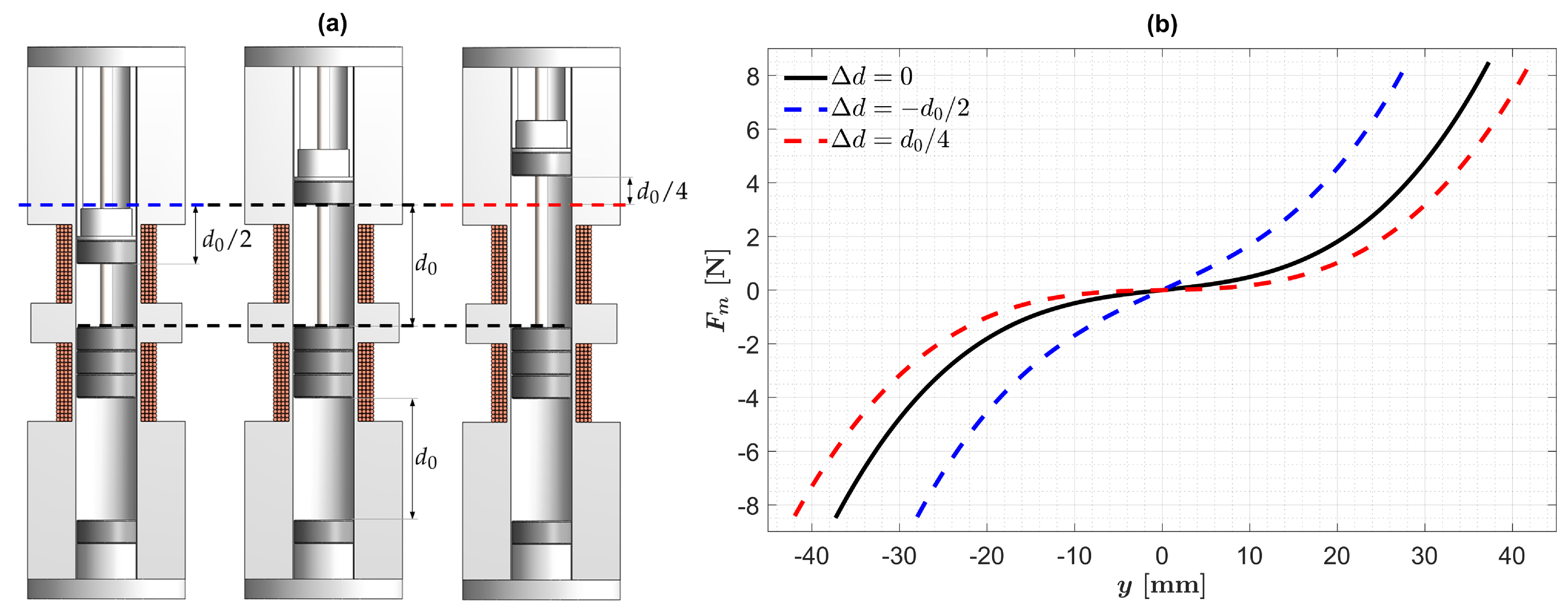
2.3. Length Variation of the Electromagnetic Harvester

The harvester length was varied within a range described by $\Delta d$. This length can be shortened by $d_0/2$ and be increased by $d_0/4$, as illustrated in Figure 2a and Equation (9).

$$-\frac{d_0}{2}⩽\Delta d⩽\frac{d_0}{4}$$

(9)

The range $\Delta d$ cannot be extended beyond $d_0/4$ and can only be shortened up to $d_0/2$ because there is no admissible force–displacement curve related to repulsive magnetic forces for larger ranges using a fitting curve only defined by two coefficients (k and $k_3$). Figure 2b presents the force–displacement non-linear behavior for the no offset scenario, as well as for shortened and stretched apparatuses along $\Delta d$.

2.4. Simulation Details

2.4.1. Details for Identification of Optimal Harvester Lengths

Intensive computation with multiple input parameter variations was performed using Matlab (v9.4, R2018a, Mathworks). The harvester length ranged from $-d_0/2⩽\Delta d⩽d_0/4$. A global search algorithm was computed using Matlab (‘GlobalSearch’ solver; ‘fmincon’ to find the minimum of the squared error function) to find parameters k and $k_3$ related to each $\Delta d$, which in turn were used to compute $\omega$ and $\beta$. The damping ratio is a parameter that also changes for different distances between non-levitating hard magnets, as presented in Equation (3a) (keeping the other parameters unchanged). The mechanical damping was defined as 0.0826 Ns/m (constant) for $\Delta d=0$, $R_l=1$ M$\mathsf{\Omega }$ and $\xi =$ 0.05, as previously defined [14]. Moreover, the harvester dynamics was analyzed for frequencies up to 100 Hz and amplitudes in the 0.1 to 8.4 m/s${}^2$ range. The mechanical and electrical dynamics were analyzed using two load resistances: 1 M$\mathsf{\Omega }$ and 188 $\mathsf{\Omega }$. The higher resistive load was defined to analyze the mechanical dynamics with negligible electrical damping. The lower resistive load was used for the maximum power transfer scenario.

The constant parameters used to carry out this detailed analysis are described in

Table 1. Constant parameters.

Parameter	Value	Units
m	0.0195	kg
$k(\Delta d=0)$	35.0396	N/m
$k(\Delta d=-d_0/2)|k(\Delta d=d_0/4)$	149.0883 | 6.7750	N/m
$k_3(\Delta d=0)$	138400	N/m${}^3$
$k_3(\Delta d=-d_0/2)|k(\Delta d=d_0/4)$	195559 | 110045	N/m${}^3$
$d_0$	37.3	mm
$\alpha$	7.752	Vs/m
$R_l$	188 $|1\times {10}^6$	$\mathsf{\Omega }$
$c_m$	0.0826	Ns/m

[14].

2.4.2. Details Used in Case Studies

The concept of self-adaptive harvesting was analyzed for multiple case studies. Analyses were conducted considering the power consumption of a real hardware apparatus composed by a ultra-low power accelerometer Bosch Sensortec BMA400 (52.2 $\mathsf{\mu }$W), ultra-low power MSP430 microcontroller (66 $\mathsf{\mu }$W) and a two-phase Faulhaber stepper motor DM0620 series (0.48 W @ 0.25 mNm). The harvester was excited with random patterns over a period from 1 h to 5 days under: (i) periodic time changes (PTC); and (ii) random time changes (RTC). Changes in random excitation patterns were established between 20 and 90 s. The number of external frequencies and amplitudes was defined between 4 and 20 times. We also defined that the accelerometer should automatically be active for 5 s. However, it will remain in the active mode until the steady excitation is reached. The accelerometer should remain inactive from 1 min to 2 h, such that no harvester length change is performed. The MSP430 microcontroller (MCU) provides the ability to enable and disable its clocks, which allows the device to be synchronized with the accelerometer. The harvester length without offsets ($\Delta d=0$) was always considered as the initial condition. First, two cases were analyzed considering: (a) 6 excitation changes under RTC for 20 h, with the accelerometer checking external excitation every 10 min; and (b) 10 excitation changes under PTC for 50 h, in which the accelerometer remains in inactive mode for 45 min. Finally, the authors investigated the average energy profile consisting of the difference between the energy harvested by the adaptive harvester (considering the energy consumption of all hardware (HW), namely sensing, processing and actuating systems) and the energy harvested by the non-adaptive architecture. This average energy profile was achieved by using multiple input scenarios to check its effectiveness over long time periods. In total, 100 frequency and amplitude patterns were randomly generated for each number of excitation changes. For example, 100 excitation sets were used for 4 excitation changes, and another 100 different excitation sets for 12 excitation changes. Moreover, for each number of excitation changes and the overall time of each case study, 100 RTC were simulated. For example, under 4 excitation changes, 100 RTC were used in the 24 h case study, and 100 different RTC in the 48 h case study.

2.5. Data Analysis

Low excitation magnitudes drive a linear behavior on the levitating magnet, resulting in a single periodic attractor for velocity (Figure 3a). However, multiple periodic attractors and hysteresis emerge as the external excitation acceleration is increased (Figure 3b) [14,27]. By consequence, the optimization here proposed was carried out by analyzing how the highest velocity ($|{\dot{y}}_M|$), achievable in both ascending ($A_t$) and descending ($D_t$) trajectories, changes for different system parameters, as defined by Equations (10) to (12).

$$A_t=\left\{\right|\dot{y}\left(\mathsf{\Omega }\right)|:\mathsf{\Omega }\in \mathbb{R}\}\mathrm{for}t\mathrm{experiments}\mathrm{when}{\mathsf{\Omega }}_{t+1}>{\mathsf{\Omega }}_t$$

(10)

$$D_t=\left\{\right|\dot{y}\left(\mathsf{\Omega }\right)|:\mathsf{\Omega }\in \mathbb{R}\}\mathrm{for}t\mathrm{experiments}\mathrm{when}{\mathsf{\Omega }}_{t+1}<{\mathsf{\Omega }}_t$$

(11)

$$|{\dot{y}}_M|=max(A_t\cap D_t)$$

(12)

The highest electric current and power, similarly defined as $|{\dot{y}}_M|$, are denoted as $I_M$ and $P_M$. The self-adaptive mechanism must then control the position of the top non-levitating magnet according to the optimized harvester length $\Delta d_{opt}$ given by:

$$\Delta d_{opt}(F_1,\mathsf{\Omega },R_l)=\Delta d:max\left|\dot{y}(F_1,\mathsf{\Omega },R_l,\Delta d)\right|,\forall \Delta d\in [-d_0/2,d_0/4]$$

(13)

The velocity, current and power gains ($VG$, $CG$ and $PG$, respectively) that will be achieved using $\Delta d_{opt}$ (in comparison with $\Delta d=0$) were computed according to Equations (14) to (16).

$$VG(F_1,\mathsf{\Omega },R_l)=\frac{|\dot{y}(F_1,\mathsf{\Omega },R_l,\Delta d=\Delta d_{opt})|}{|\dot{y}(F_1,\mathsf{\Omega },R_l,\Delta d=0)|}$$

(14)

$$CG(F_1,\mathsf{\Omega },R_l)=\frac{I(F_1,\mathsf{\Omega },R_l,\Delta d=\Delta d_{opt})}{I(F_1,\mathsf{\Omega },R_l,\Delta d=0)}$$

(15)

$$PG(F_1,\mathsf{\Omega },R_l)=\frac{P(F_1,\mathsf{\Omega },R_l,\Delta d=\Delta d_{opt})}{P(F_1,\mathsf{\Omega },R_l,\Delta d=0)}$$

(16)

3. Results

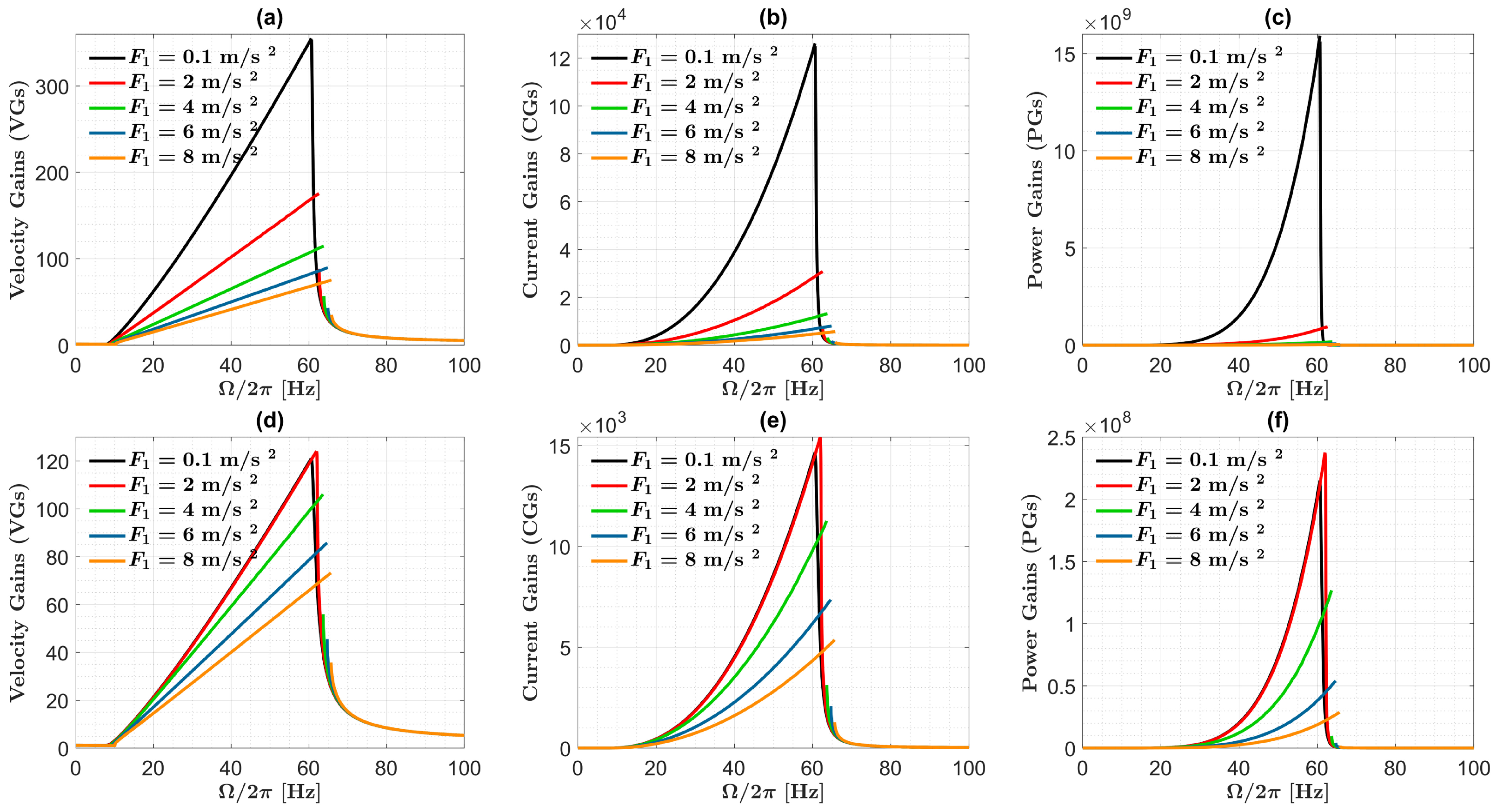
3.1. Identification of Optimal Harvester Lengths and Related Performance Gains

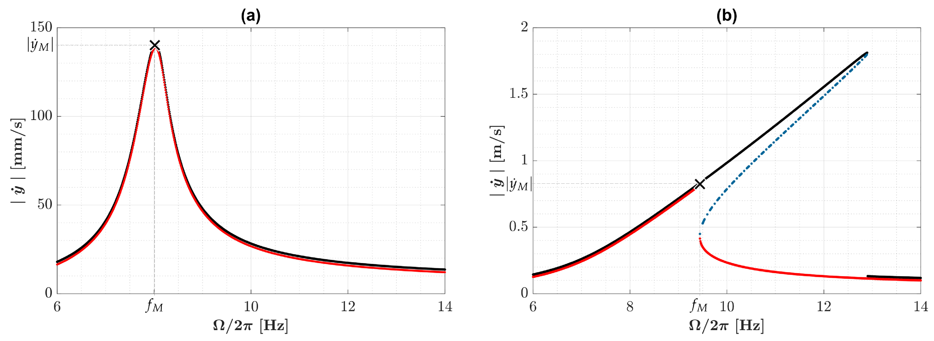
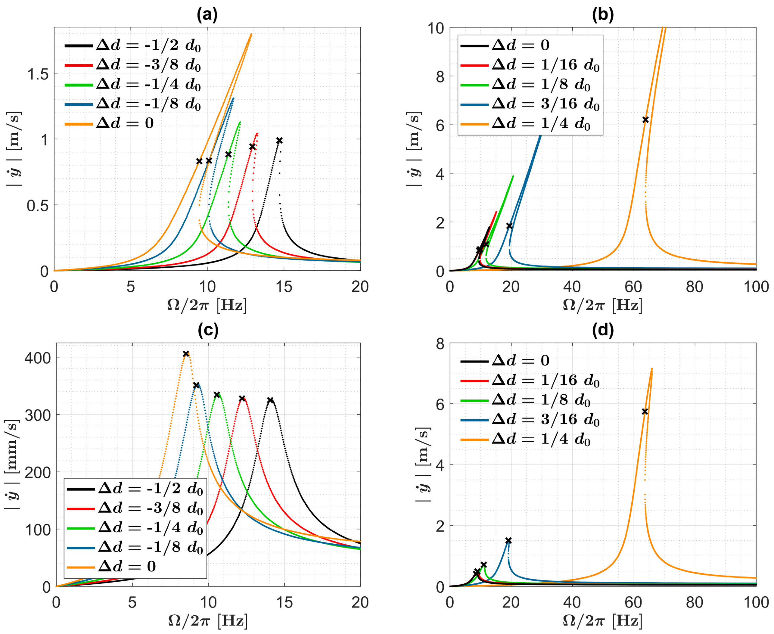
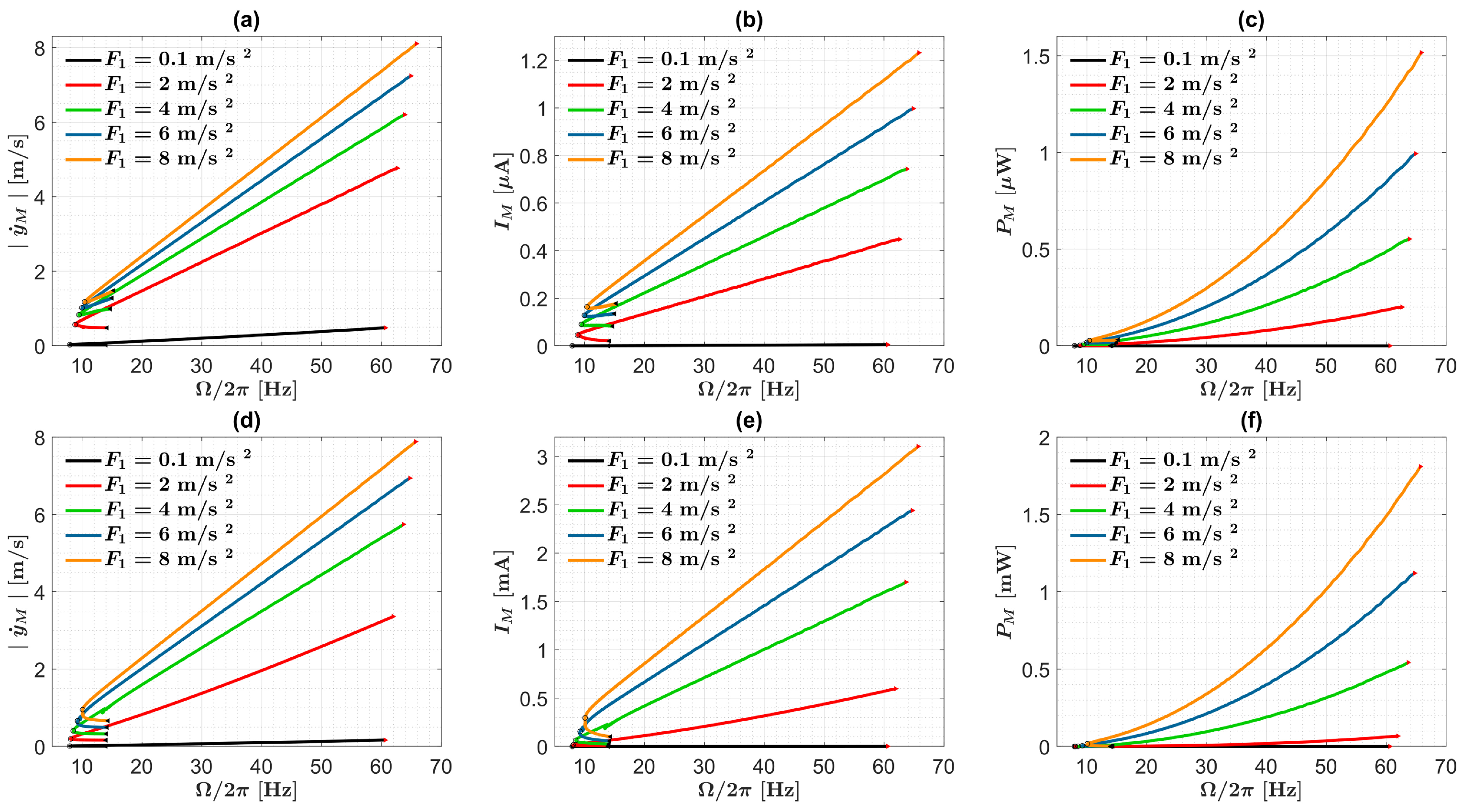
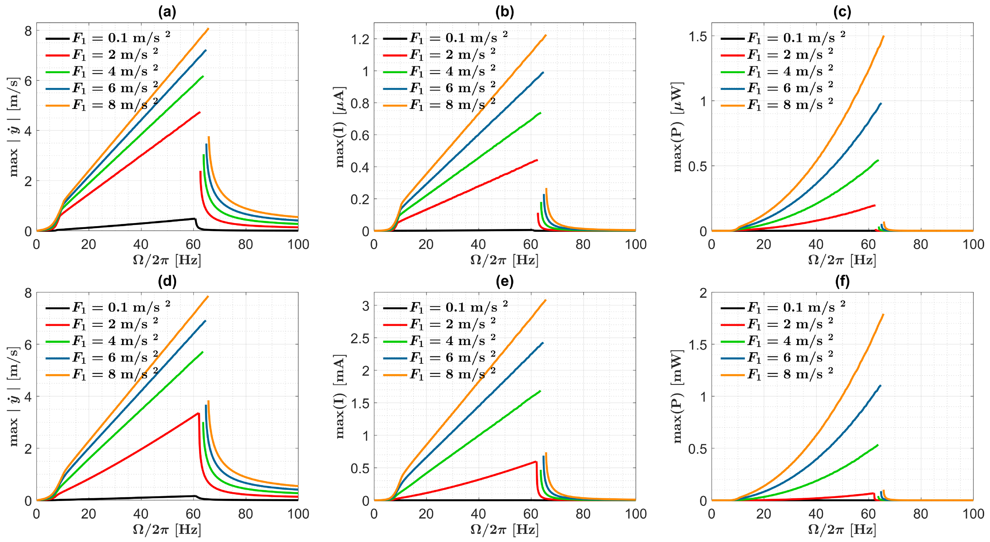
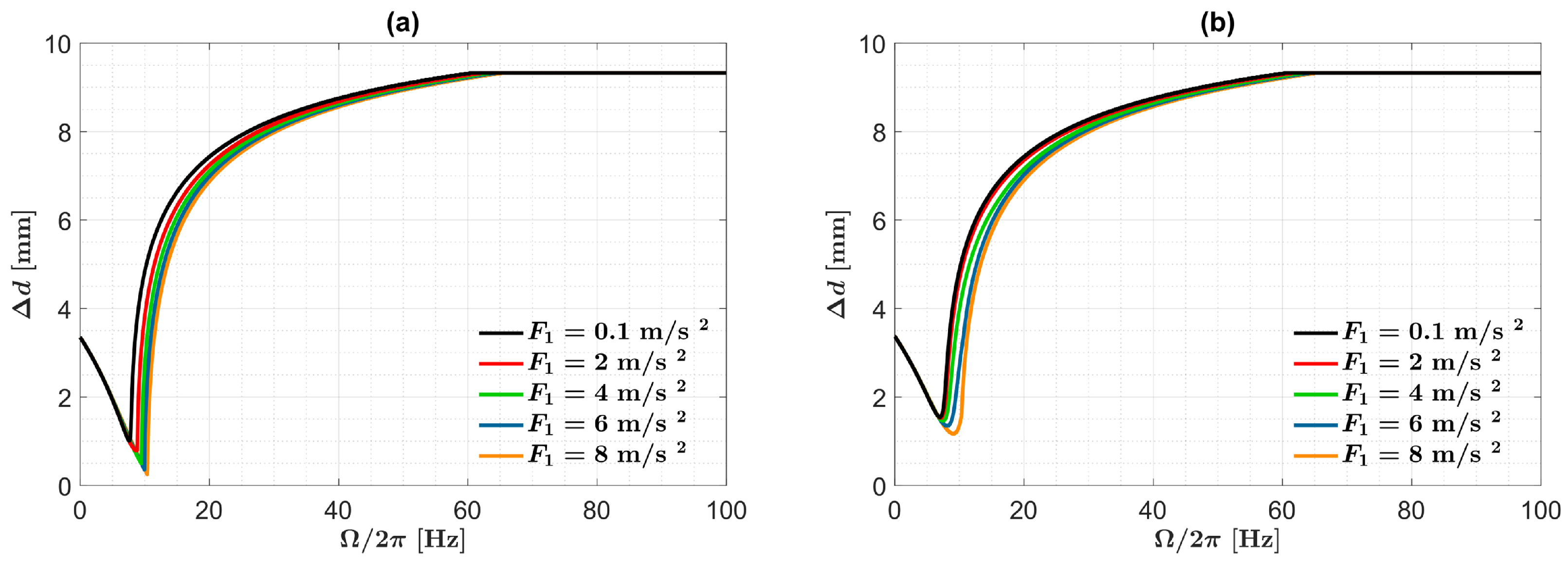
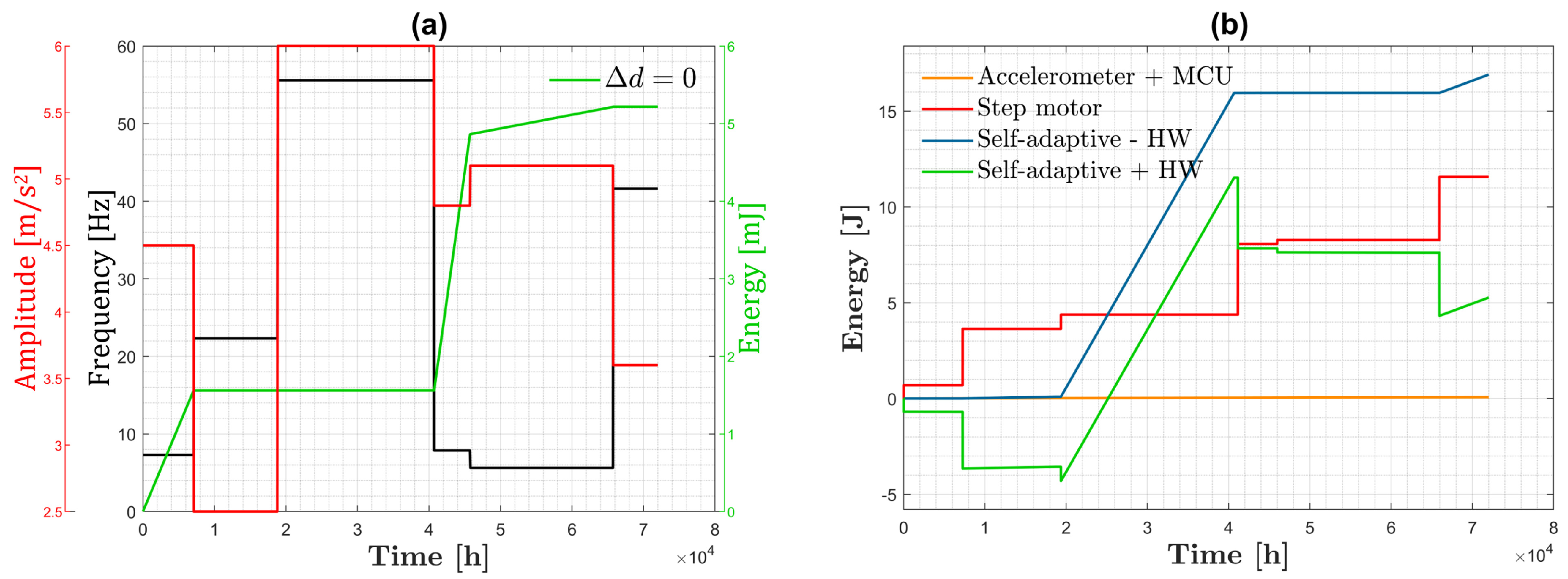
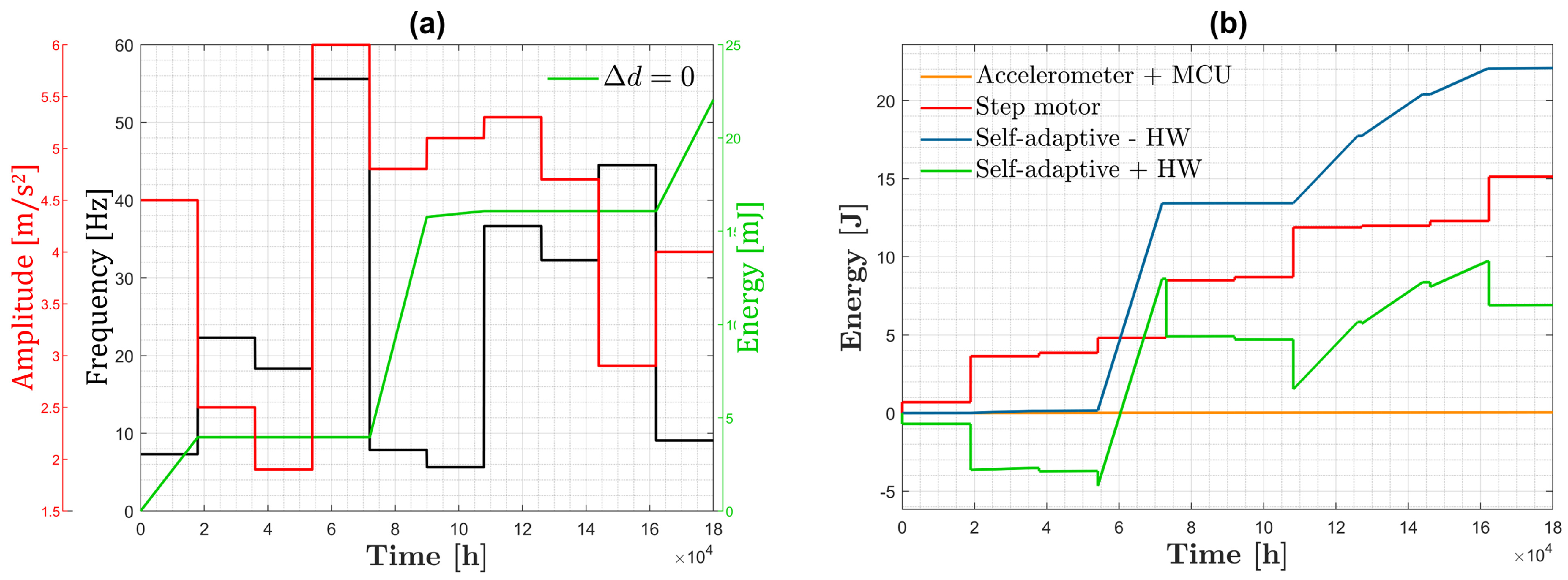
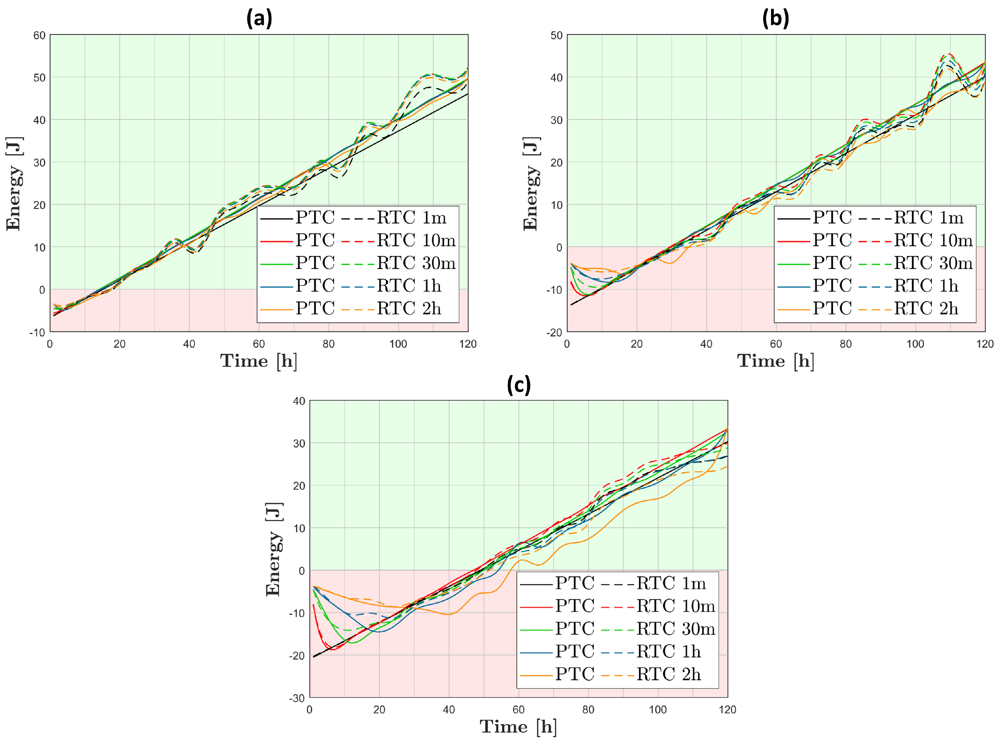
The concept of self-adaptive energy harvesting requires the identification of the optimal distance between non-levitating magnets for each excitation. Such a task firstly requires us to find the relative velocity response and related $|{\dot{y}}_M|$ for distinct harvester lengths in the range $-d_0/2⩽\Delta d⩽d_0/4$ (Figure 4). Under 1 M$\mathsf{\Omega }$ load and 4 m/s${}^2$ of excitation, slight decreases in $|{\dot{y}}_M|$ and in related frequencies are observed as $\Delta d$ is increased from $-d_0/2$ to 0, as illustrated in Figure 4a: $\Delta |{\dot{y}}_M|$ is 158 mm/s for frequency changes of 5.2 Hz. This behavior does not occur for the maximum power transfer scenario (Figure 4c): $|{\dot{y}}_M|$ increases as related frequencies decrease, 81 mm/s obtained for $\Delta |{\dot{y}}_M|$ and frequency changes of 5.5 Hz. However, considerable increases in both $|{\dot{y}}_M|$ and related frequencies are noticed when $\Delta d$ increases from 0 to $d_0/4$ under both loads, as shown in Figure 4b,d. As expected, the use of the 1 M$\mathsf{\Omega }$ load resistance provides higher $|{\dot{y}}_M|$ values when compared to the 188 $\mathsf{\Omega }$ load resistance. Due to the significant influence of the electrical damping coefficient when the lowest load is used, the dynamics of the levitating magnet barely have coexisting solutions (Figure 4c,d). Increasing $\Delta d$ in the range from 0 to $d_0/4$ results in $\Delta |{\dot{y}}_M|$ up to 5.4 m/s and frequency changes up to 54.4 Hz for the open-circuit scenario, and $\Delta |{\dot{y}}_M|$ up to 5.3 m/s and frequency changes up to 55.1 Hz when the maximum power transfer scenario is achieved.

Figure 5 exhibits the overall behavior of the $|{\dot{y}}_M|$, $I_M$ and $P_M$ for varying harvester lengths in the range $-d_0/2⩽\Delta d⩽d_0/4$ and excitations from 0.1 to 8.4 m/s${}^2$. Regardless of the excitation and load resistance, the frequency values related to $|{\dot{y}}_M|$, $I_M$ and $P_M$ express similar behavior as the harvester length is shortened ($-d_0/2⩽\Delta d⩽0$). Although these frequencies always decrease for increasing $\Delta d$, $|{\dot{y}}_M|$, $I_M$ and $P_M$ patterns are excitation- and load-dependent. Concerning the maximum power transfer required, unexpected frequency decreases associated with $|{\dot{y}}_M|$ and $I_M$ increases occur as $\Delta d$ is increased from $-d_0/2$ up to 0. The maximum $\Delta |{\dot{y}}_M|$ and $\Delta I_M$ are 290 mm/s and 194 $\mathsf{\mu }$A for frequency changes of around 5.1 Hz. These results are quite relevant as: (i) low-frequency vibrations are particularly abundant; (ii) the reduction in size is a critical requirement of self-powered electrical microsystems, mainly for new technological trends that aim to implement multifunctional and intelligent capabilities. These patterns significantly differ when the harvester length is increased from 0 to $\Delta d=d_0/4$. Significant increases in $|{\dot{y}}_M|$, $I_M$ and $P_M$ and related frequencies are expected as $\Delta d$ is increased. Around a 7-fold increase in the frequency is observed for increases in $|{\dot{y}}_M|$ that range between 17-fold increases and 8-fold increases as excitation is increased from 0.1 m/s${}^2$ to 8 m/s${}^2$. Similar frequency increases are obtained for increases in $I_M$ that range between 41-fold increases and 11-fold increases when the same excitations are applied. Similar analyses of $P_M$ reveal that it ranges between 1558-fold increases and 113-fold increases. Therefore, the harvester performance is significantly improved by frequency increases. The lowest frequencies related to $|{\dot{y}}_M|$, $I_M$ and $P_M$ are achieved for the harvester length without offsets ($\Delta d=0$). In this $\Delta d=0$ scenario, higher magnitude excitations drive higher frequencies, although these changes are confined to the narrow range between 7.9 and 10.1 Hz. $P_M$ behaves slightly differently from $I_M$ (Figure 5c,f) as $P_M$ is proportional to the square of $I_M$. Even so, the overall trend of $P_M$ is similar to $|{\dot{y}}_M|$ and $I_M$.

Detailed analyses allowed us to identify a passband defining the range of excitation frequencies that will provide optimal levitating magnet velocities, electric currents and power. Figure 6 shows the highest values of $|\dot{y}|$, I and P achievable by this electromagnetic harvester, which in turn were used to identify the best harvester lengths. The linear patterns of $|{\dot{y}}_M|$, $I_M$ and $P_M$ observed in Figure 5 for $0⩽\Delta d⩽d_0/4$ are included within the best achievable values, regardless of the excitation and load resistance. This occurs for approximate frequencies between 9 and 63 Hz (the higher the excitation, the higher this cut-off frequency). Non-linear behaviors emerge for excitation frequencies lower than ≈9 Hz and higher than ≈63 Hz: the highest magnitudes of the non-levitating velocity, current and power significantly decrease as the excitation frequencies surpass the 9–63 Hz passband. Several discontinuities are also observed for excitation frequencies around 63 Hz. These occur as multiple attractors emerge when $\Delta d=d_0/4$, which were discarded as established in Section 2.5.

The best harvester lengths that provide the best patterns of the relative velocity of the levitating magnet, electric current and power are illustrated in Figure 7. The optimal offset $\Delta d$, which maximizes the harvester performance, exhibits highly non-linear patterns as a function of the excitation frequency. Similar patterns are observed for very different load resistances. Interestingly, the optimal offset $\Delta d$ is always positive, regardless of the excitation frequency and load. The best $\Delta d$ for very low frequencies is 3.4 mm. After a quasi-linear decreasing pattern up to ≈9 Hz, the minima $\Delta d$ are lower than 1 and 1.5 mm for 188 $\mathsf{\Omega }$ and 1 M$\mathsf{\Omega }$, respectively. Differently, an optimal offset increase is noticed for excitation frequencies exceeding 9 Hz until $\Delta d$ reaches the maximum $\Delta d=d_0/4$ mm (≈63 Hz).

In comparison with non-adaptive operation, gains in terms of velocity, current and power will be obtained when the self-adaptive electromagnetic harvester adapts its architecture as variations in the excitation patterns occur (Figure 8). The most significant gains are exhibited in the range 9–63 Hz (quasi-linear increasing patterns) and for lower excitation amplitudes. For the open-circuit scenario, gains are exhibited up to 355, $1.3\times {10}^5$ and $1.6\times {10}^{10}$ for $VG$, $CG$ and $PG$, respectively; different gains are predicted for the maximum power transfer scenario: 124, $1.5\times {10}^4$ and $2.4\times {10}^8$ for $VG$, $CG$ and $PG$, respectively. Both scenarios provide a minimum gain of 1. Lower gains are expected when the excitation amplitudes are increased. Indeed, when the open-circuit scenario is analyzed, a $VG$ is provided between 75 and 355 as the excitation decreases from 8 m/s${}^2$ to 0.1 m/s${}^2$; concerning current and power, gains between 5676 and 1.3 × 10${}^5$ and between $3.2\times {10}^7$ and $1.6\times {10}^{10}$, respectively, are ensured for decreasing excitations. When the harvester is harvesting the maximum power transfer, a $VG$ is provided between 73 and 121 as the excitation decreases from 8 m/s${}^2$ to 0.1 m/s${}^2$; moreover, $CG$ and $PG$ are achieved in the range 5364–$1.5\times {10}^4$ and in the range $2.9\times {10}^7$–$2.1\times {10}^8$, respectively, for the same decreasing excitations. Notice that the several discontinuities observed for excitation frequencies around 63 Hz have identical cause, as previously described (Figure 6).

3.2. Case Studies

Figure 9 shows a case study where the harvester is excited with RTC and six different excitations. Random frequencies and amplitudes are illustrated on the left y-axis. The energy dynamics with and without self-adaptive length are illustrated in Figure 9a,b respectively. Energy harvesting using fixed top non-levitating magnets provides 5.2 mJ for the 20 h experiment, while the automatic adaptation of the harvester provides 16.9 J. During the same period, the accelerometer and MCU energy demand were only 70.9 mJ, but the step motor required 11.6 J. Considering this 68.6% energy decrease, the self-adaptive system, including the related HW, was able to harvest 5.3 J (99.9% increase compared to the $\Delta d=0$ scenario). As expected, the significant impact of the energy demanded by the hardware is observed, mostly by the actuation system. Concerning the non-adaptive harvester (Figure 9a), the highest energy rates (in descending order) occur in the following time ranges: 11.3–12.7 h, 0–2 h and 12.7–18.3 h. The harvested energy rate decays significantly as the excitation frequency is separated from $f_M$, which in turn is related to the excitation amplitude (as highlighted in Figure 3). The adaptive harvester provides higher energy rates when time lies between 5.2 and 11.3 h, as well as between 18.3 and 20 h, as expected from Figure 6. The energy dynamics for the self-adaptive harvester when $t=11.3$ h keeps growing but at a much lower rate as the excitation changes, although this occurs as the sensor only monitors such variation 7.8 min later.

Concerning the second case study, whose results are illustrated in Figure 10, the non-adaptive harvester was only able to generate 22 mJ. Despite being only 2.5 times longer than the previous case study, the energy gains are 4.2 times higher. However, the self-adaptive harvester (including all HW) was able to generate 6.9 J over 50 h. The highest rate of adaptive harvested energy occurs during 40% of the case study, namely in the ranges between 15 and 20 h and between 30 and 45 h, as illustrated in Figure 10b. Again, the energy demand to power both the sensing and processing systems (39.6 mJ) is almost negligible compared to the energy required to power the step motor (15.1 J). The hardware from the adaptive mechanism consumes 68.7% of the generated energy. When $t=35$ h and $t=40$ h, the system takes, respectively, 18.3 and 35 min to perform the length adaptation, as the accelerometer only monitors excitation changes every 45 min. The motor that changes the position of the top non-levitating magnet was energized for 24.1 and 31.5 s for the 20 and 50 h experiments, respectively. For these scenarios, energy gains were only achieved after 7 and 17 h of continuous operation.

Concerning the average energy profile for multiple input scenarios, positive energy gains are always achieved for 5-day experiments, as illustrated in Figure 11. A similar energetic trend of the instrumented harvester is observed, although positive performance occurred after between 18 and 58 h. The less the excitation changes, the higher the average energy generated, because a lower energy is required to adjust the harvester length (during a 5-day experiment, and for a number of different excitations reduced from 12 to 4, the average energy increases by around 16.5%). A positive trend is observed for all average positive energy values (green regions in Figure 11), although this trends starts occurring even for negative values (red regions). Despite presenting very identical dynamics, the average energy profile tends to evolve more linearly with PTC than with RTC. On one hand, it is worthwhile to adapt the harvester length as quickly as possible for few excitation changes (using shorter inactive accelerometer times), resulting in higher energy rates in shorter times. On the other hand, under reduced operating scenarios, as the number of excitation changes increases, higher energy will be generated if the sensor is inactive for longer time periods. The energy gains are generally higher for long operating scenarios, when the accelerometer regularly checks the excitation patterns (shorter inactive times). The average energy profile dynamics for 20 different excitations (Figure 11c) is the best up to 27 h of operation (under 2 h of inactive sensing time), as the instrumented harvester adapts its length fewer times. Nevertheless, the worst energy profile after 27 h operation was obtained for the same conditions (Figure 11c).

4. Discussion and Conclusions

In this study, we provide a unique insight into the new concept of the electromagnetic harvester, which is able to maximize the energy performance by means of a sophisticated method that controls the distance between non-levitating hard magnets as variations in the excitation patterns occur. This length-dependent harvester performance must be further explored to develop harvesters that automatically are tuned according to the frequency and magnitude of the mechanical excitation. The concept was analytically analyzed and the optimal harvester lengths ($\Delta d$) for different excitation patterns under two load resistances were identified.

Some efforts have been made so far to optimize the performance of electromagnetic energy harvesters using magnetic levitation architectures by analyzing the effect of varying (i) the materials to manufacture the container, shaft and spacer; (ii) the number, dimensions and mass of the inertial magnet(s); and (iii) the number of turns, width, height and position of the coil [5]. These approaches were conducted for optimization prior to fabrication and for particular excitations, but disregarding the optimization throughout their operation. Up to now, no effective technological solution had been proposed to optimize such harvesters for time-varying excitations [5]. Nevertheless, this methodology can be used in harvesters with either a fixed distance between non-levitating magnets (geometrically projected to a priori known excitations) or variable distances (as a function of time-variating excitation patterns). Nevertheless, gains related to electric current and power can be achieved in comparison with non-adaptive operation. Moreover, harvesters designed with self-adaptive mechanisms will also require low maintenance and ensure non-intermittent harvesting. All these advantages suggest the possibility of optimized operation in a wide range of scenarios (loads, mechanical excitations, dampings, etc.).

The used analytical model captures the fundamental dynamics of the mechanical–electric transduction mechanism of these electromagnetic harvesters [14]. It was experimentally validated, even if the following assumptions were considered: (i) both the magnetic field and the electromechanical coefficient are constants; (ii) the coil inductance is not introduced in the electrical dynamics; (iii) it is only valid for limited $d_0$ and $\Delta d$ variations; and (iv) magnets are coaxially positioned. Hence, experimental results are not expected to differ from these here reported if similar architectures are used. The excitation patterns and the total energy required to power the step motor are the most influential performance parameters. Concerning the first two case studies, energy gains were obtained around after 35% of the overall operation time. In the worst case scenario for multiple input characteristics (Figure 11), around 48% of operation time is required to achieve energy gains. Nevertheless, as the overall operation time increases, the operation time without energy gains approaches zero. These results are impactful because many self-powered technologies using energy harvesting operate for many years, such as ocean wave energy harvesters and bioelectronic implantable medical devices.

Finally, further research must be conducted to evaluate the effectiveness of this radically new harvester comprising multiple coils and multiple levitating magnets [5]. A study must be also conducted for large-scale harvesters. The energy performance must be analyzed for tri-dimensional motions of instrumented harvesters, such that realistic excitation patterns of external mechanical power sources can be used.

References

1. EIA. International Energy Outlook 2016 whith Projections to 2040; 2016; p. 276. Available online: https://www.osti.gov/biblio/1296780 (accessed on 20 March 2022).
2. Larsson, S.; Fantazzini, D.; Davidsson, S.; Kullander, S.; Höök, M. Reviewing electricity production cost assessments. Renew. Sustain. Energy Rev. 2014, 30, 170–183. [Google Scholar] [CrossRef] [Green Version]
3. Sovacool, B.K. The intermittency of wind, solar, and renewable electricity generators: Technical barrier or rhetorical excuse? Util. Policy 2009, 17, 288–296. [Google Scholar] [CrossRef]
4. Elliott, D. A balancing act for renewables. Nat. Energy 2016, 1, 15003. [Google Scholar] [CrossRef]
5. Carneiro, P.; Soares dos Santos, M.P.; Rodrigues, A.; Ferreira, J.A.; Simões, J.A.; Marques, A.T.; Kholkin, A.L. Electromagnetic energy harvesting using magnetic levitation architectures: A review. Appl. Energy 2020, 260, 114191. [Google Scholar] [CrossRef] [Green Version]
6. dos Santos, M.P.S.; Ferreira, J.A.F.; Simões, J.A.O.; Pascoal, R.; Torrão, J.; Xue, X.; Furlani, E.P. Magnetic levitation-based electromagnetic energy harvesting: A semi-analytical non-linear model for energy transduction. Sci. Rep. 2016, 6, 18579. [Google Scholar] [CrossRef]
7. Dewan, A.; Ay, S.U.; Karim, M.N.; Beyenal, H. Alternative power sources for remote sensors: A review. J. Power Sources 2014, 245, 129–143. [Google Scholar] [CrossRef]
8. Beeby, S.P.; Tudor, M.J.; White, N.M. Energy harvesting vibration sources for microsystems applications. Meas. Sci. Technol. 2006, 17, 175–195. [Google Scholar] [CrossRef]
9. Teng, X.F.; Zhang, Y.T.; Poon, C.C.Y.; Bonato, P. Wearable medical systems for p-health. IEEE Rev. Biomed. Eng. 2008, 1, 62–74. [Google Scholar] [CrossRef]
10. Dos Santos, M.P.; Marote, A.; Santos, T.; Torrão, J.; Ramos, A.; Simões, J.A.; Da Cruz E Silva, O.A.; Furlani, E.P.; Vieira, S.I.; Ferreira, J.A. New cosurface capacitive stimulators for the development of active osseointegrative implantable devices. Sci. Rep. 2016, 6, 30231. [Google Scholar] [CrossRef] [Green Version]
11. Soares dos Santos, M.P.; Coutinho, J.; Marote, A.; Sousa, B.; Ramos, A.; Ferreira, J.A.; Bernardo, R.; Rodrigues, A.; Marques, A.T.; Cruz e Silva, O.A.; et al. Capacitive technologies for highly controlled and personalized electrical stimulation by implantable biomedical systems. Sci. Rep. 2019, 9, 5001. [Google Scholar] [CrossRef] [Green Version]
12. Peres, I.; Rolo, P.; Ferreira, J.A.F.; Pinto, S.C.; Marques, P.A.A.P.; Ramos, A.; Soares dos Santos, M.P. Multiscale Sensing of Bone-Implant Loosening for Multifunctional Smart Bone Implants: Using Capacitive Technologies for Precision Controllability. Sensors 2022, 22, 2531. [Google Scholar] [CrossRef] [PubMed]
13. Alanne, K.; Cao, S. An overview of the concept and technology of ubiquitous energy. Appl. Energy 2019, 238, 284–302. [Google Scholar] [CrossRef]
14. Mann, B.P.; Sims, N.D. Energy harvesting from the nonlinear oscillations of magnetic levitation. J. Sound Vib. 2009, 319, 515–530. [Google Scholar] [CrossRef] [Green Version]
15. Harne, R.L.; Schoemaker, M.E.; Dussault, B.E.; Wang, K.W. Wave heave energy conversion using modular multistability. Appl. Energy 2014, 130, 148–156. [Google Scholar] [CrossRef]
16. Stoutenburg, E.D.; Jacobson, M.Z. Reducing offshore transmission requirements by combining offshore wind and wave farms. IEEE J. Ocean. Eng. 2011, 36, 552–561. [Google Scholar] [CrossRef]
17. Berdy, D.F.; Valentino, D.J.; Peroulis, D. Kinetic energy harvesting from human walking and running using a magnetic levitation energy harvester. Sensors Actuators Phys. 2015, 222, 262–271. [Google Scholar] [CrossRef]
18. Geisler, M.; Boisseau, S.; Perez, M.; Gasnier, P.; Willemin, J.; Ait-Ali, I.; Perraud, S. Human-motion energy harvester for autonomous body area sensors. Smart Mater. Struct. 2017, 26, 12. [Google Scholar] [CrossRef]
19. Masoumi, M.; Wang, Y. Repulsive magnetic levitation-based ocean wave energy harvester with variable resonance: Modeling, simulation and experiment. J. Sound Vib. 2016, 381, 192–205. [Google Scholar] [CrossRef] [Green Version]
20. Zhang, C.L.; Chen, W.Q. A wideband magnetic energy harvester. Appl. Phys. Lett. 2010, 96, 123507. [Google Scholar] [CrossRef]
21. Jang, S.J.; Kim, I.H.; Jung, H.J.; Lee, Y.P. A tunable rotational energy harvester for low frequency vibration. Appl. Phys. Lett. 2011, 99, 134102. [Google Scholar] [CrossRef]
22. Zhu, D.; Tudor, M.J.; Beeby, S.P. Strategies for increasing the operating frequency range of vibration energy harvesters: A review. Meas. Sci. Technol. 2010, 21, 29. [Google Scholar] [CrossRef]
23. Harne, R.L.; Wang, K.W. A review of the recent research on vibration energy harvesting via bistable systems. Smart Mater. Struct. 2013, 22, 12. [Google Scholar] [CrossRef]
24. Nguyen, S.D.; Halvorsen, E. Nonlinear springs for bandwidth-tolerant vibration energy harvesting. J. Microelectromech. Syst. 2011, 20, 1225–1227. [Google Scholar] [CrossRef]
25. Siddique, A.R.M.; Mahamud, S.; Heyst, B.V. A comprehensive review on vibration based micro power generators using electromagnetic and piezoelectric transducer mechanisms. Energy Convers. Manag. 2015, 106, 728–747. [Google Scholar] [CrossRef]
26. Struwig, M.N.; Wolhuter, R.; Niesler, T. Nonlinear model and optimization method for a single-axis linear-motion energy harvester for footstep excitation. Smart Mater. Struct. 2018, 27, 125007. [Google Scholar] [CrossRef] [Green Version]
27. Wang, W.; Cao, J.; Zhang, N.; Lin, J.; Liao, W.H. Magnetic-spring based energy harvesting from human motions: Design, modeling and experiments. Energy Convers. Manag. 2017, 132, 189–197. [Google Scholar] [CrossRef]
Figure 1. (a) Three-dimensional section view of the self-adaptive harvester; (b) platform to experimentally validate the concept of self-adaptive electromagnetic energy harvesting; (c) schematic representation of the electromagnetic harvester and electric circuit diagram; and (d) diagram representing a control approach only using data from the excitation dynamics. Legend: 1a–adaptive non-levitating magnet; 1b–levitating magnets; 1c–non-levitating magnet; 2–coil; 3–magnet–rod coupling; 4, 48–lid; 5, 7, 11, 16, 24, 29, 32, 33, 35, 37, 41, 46–screw; 6–accelerometer; 8–aluminium board; 9–accelerometer housing; 10, 15, 26, 28, 31, 36, 45–support; 12–container; 13–inertial guiding rod; 14, 25, 47–sleeve bearing; 17, 18–tube–nut fastener; 19–lock nut; 20–tube; 21–spacer; 22, 44–guiding shaft; 23–anti-vibration fastener; 27–sensor nut; 30–ultrasonic sensor; 34–stepper motor; 38–stud; 39–motor–spindle coupling; 40–sliding nut; 42–extremity of inertial mass; 43–trapezoidal spindle screw; 49–tube–magnet coupling.
Machines 10 00414 g001
Figure 2. (a) Variation in the harvester length from d 0 / 2 Δ d d 0 / 4 (windings were not considered to simplify this illustration); (b) force–displacement curves when the harvester variation length is: neglected ( Δ d = 0 , black solid line); shortened to Δ d = d 0 / 2 (blue dashed line); and extended to Δ d = d 0 / 4 (red dashed line).
Machines 10 00414 g002
Figure 3. Relative velocity response for Δ d = 0 , R l = 1 M Ω and the following excitation amplitudes: (a) 0.5 m/s 2 and (b) 4 m/s 2 . The behavior due to the non-linear phenomenon for upward ( A t ) and downward ( D t ) frequency sweeps is identified by the black and red solid lines, respectively (stable periodic solutions), while the blue dashed line illustrates unstable periodic solutions; the maximum velocities considered ( | y ˙ M | ) are identified with black crosses.
Machines 10 00414 g003
Figure 4. Relative velocity responses according to the external excitation frequencies under different harvester lengths bounded by: (a) d 0 / 2 Δ d 0 , R l = 1 M Ω ; (b) 0 Δ d d 0 / 4 , R l = 1 M Ω ; (c) d 0 / 2 Δ d 0 , R l = 188 Ω ; and (d) 0 Δ d d 0 / 4 , R l = 188 Ω . The excitation amplitude was defined as 4 m/s 2 and | y ˙ M | are identified with black crosses.
Machines 10 00414 g004
Figure 5. Optimal levitating magnet velocities, electric currents and power for five excitation amplitudes when Δ d changes from − d 0 /2 to d 0 /4: (ac) | y ˙ M | , I M and P M for R l = 1 M Ω ; (df) | y ˙ M | , I M and P M for R l = 188 Ω . Δ d = 0 is identified by a black circle dot.
Machines 10 00414 g005
Figure 6. Optimal performance of the self-adaptive harvester using the optimal lengths computed for five excitation amplitudes: (ac) | y ˙ M | , I M and P M for R l = 1 M Ω ; (df) | y ˙ M | , I M and P M for R l = 188 Ω .
Machines 10 00414 g006
Figure 7. Optimal harvester lengths for five excitation amplitudes under: (a) R l = 1 M Ω and (b) R l = 188 Ω .
Machines 10 00414 g007
Figure 8. Performance gains achieved by the self-adaptive harvester for five excitation amplitudes: (ac) V G , C G and P G for R l = 1 M Ω ; (df) V G , C G and P G for R l = 188 Ω .
Machines 10 00414 g008
Figure 9. (a) Six random frequency and amplitude patterns under RTC on the left y-axis and correspondent harvested energy on the right y-axis for non-adaptive harvester; (b) energy demand from sensing, processing and actuation systems—self-adaptive harvested energy neglecting the hardware consumption, as well as considering the hardware consumption. The accelerometer inactivation time was set to 10 min.
Machines 10 00414 g009
Figure 10. (a) Ten random frequency and amplitude patterns under PTC on the left y-axis and correspondent harvested energy on the right y-axis for non-adaptive harvester; (b) energy demand from sensing, processing and actuation systems—self-adaptive harvested energy neglecting the hardware consumption, as well as considering the hardware consumption. The accelerometer inactivation time was set to 45 min.
Machines 10 00414 g010
Figure 11. Average energy profile vs. simulation time for five sensing inactive times under (a) 4 excitations; (b) 12 excitations; and (c) 20 excitations. The behavior due to PTC and RTC is identified by the solid and dashed lines, respectively.
Machines 10 00414 g011