1. Introduction
For a single rigid-body, there was multitudinous literature having investigated attitude control [
1,
2] or trajectory control [
3,
4,
5]. However, when a task of high efficiency and large scale is required, an individual rigid-body (e.g., an aircraft or a robot) could not be unable to meet the specific requirements in some situations. Because of the high efficiency and the reliability of a multi-agent system (MASs), a group of multiple rigid-bodies can provide a new way to solve the complicated tasks. During the last two decades, cooperative control of multi-agent systems (MASs) has drawn increasing attention, which could be attributed to its widespread applications in various fields. For example, attitude and position synchronization for spacecraft formation flying [
6,
7,
8], attitude consensus tracking for multiple rigid-bodies [
9,
10,
11], distributed formation flying for a team of unmanned aerial vehicles (UAVs) [
12,
13,
14,
15], distributed formation control for a set of mobile robots [
16,
17], and cooperative guidance for a group of interceptors [
18,
19,
20]. Among those works, the consensus control task, aiming at achieving an agreement among agents by using local information interaction, is often an elementary problem. Thus, numerous literature works have studied this problem recently.
In Ref. [
21], an attitude consensus control scheme was proposed for a group of spacecraft attitude tracking without angular-velocity measurements. The control torques are naturally bounded, and the bounds of control torque could be arbitrarily prescribed through the control gains. In Ref. [
22], the output consensus problem was investigated for a class of high-order nonlinear MASs. Based on a system state transformation, a distributed linear-like control law with a dynamic gain was proposed by using the agent and its neighbors output information. In addition, the orders of all considered agents could be different. In Ref. [
23], a new distributed observer-type reduced-order output-feedback consensus control law was proposed for homogeneous linear MASs. System state consensus was achieved, and the consensus conditions were presented. Regarding the consensus control problem, convergence speed is an important performance reflecting effectiveness of the proposed algorithm. The above-mentioned literature can only achieve asymptotic stability, which means that the convergence time is actually infinite. By contrast, finite-time stability implies faster settling-time and excellent robustness against various uncertainties.
Hence, a finite-time consensus control algorithm could attract more attention. In Ref. [
24], a decentralized observer and a distributed observer were presented to estimate velocity state of each agent and acceleration of the leader, respectively. Based on the two finite-time observers, a distributed finite-time control law was proposed for multiple spacecraft formation flying with a virtual-leader. With the help of homogeneity theory, semi-global finite-time stability of the overall closed-loop system was rigorously proved. However, the robustness against uncertainties for each spacecraft is not taken into account. The authors of Ref. [
25] proposed two robust distributed finite-time consensus protocols for MASs with double-integrator dynamics, in which leaderless and leader-following scenarios were considered, respectively. In the leader-following situation, a distributed finite-time observer was proposed to estimate velocity state of the leader. However, the presented control law is only for single-input single-output (SISO) systems. That is to say, for any node, the used mathematic model is a SISO system. In Ref. [
26], the leader-following consensus problem was investigated for a class of second-order MASs. Based on a prescribed finite-time observer and a time-varying disturbance observer, a novel composite leader-following consensus control law was proposed. Both matched and mismatched disturbances could strongly be suppressed. It is worth pointing out that there is an obvious disadvantage of a finite-time consensus control law. If the initial condition is far away from the origin, the convergence speed of a finite-time algorithm is slower than an exponential convergence algorithm.
A solution to remove that drawback of a finite-time consensus control is the fixed-time consensus control. A recent review paper of this research orientation was given in Ref. [
27]. In Ref. [
28], based on a distributed fixed-time observer, two novel distributed fixed-time control laws were proposed for MASs with uncertainties acting on each agent. To mitigate the chattering effect, a boundary-layer method was employed, and a saturation-function was used to take the place of signum-function when the tracking errors enter the boundary-layer. Therefore, some performance reductions were paid for the expense of using the saturation-function. In Ref. [
29], two fixed-time sliding-mode observers were presented at the beginning. Based on the two fixed-time observers, two distributed fixed-time attitude consensus control laws were proposed for a group of multiple spacecrafts. Required measurement of angular velocity was used in the first algorithm, whereas this requirement was removed in the second. With the aid of the two control laws, all spacecrafts are able to track a time-varying reference attitude, which is only available to a subset of the spacecrafts.
This work considers the fixed-time attitude consensus tracking control problem for a group of multiple rigid-bodies. Compared with the existing works of fixed-time consensus control law, the main contributions can be summarized as follows:
A robust exact distributed fixed-time observer (REDFTO) is proposed to estimate velocity state of the virtual-leader. Settling-time of the dynamics of estimation error is independent of the initial conditions. The required computational burden of the REDFTO is less than some of the existing results [
28,
29], whereas fixed-time convergence of the estimation error to the origin could be guaranteed.
Based on the presented REDFTO, a distributed fixed-time consensus tracking control (DFCTC) law is proposed for leader–follower MASs. Fixed-time convergence of the consensus tracking errors is proved by means of a modified back-stepping technique [
30]. In the presence of lumped time-varying uncertainty acting on each agent, compared with the result [
31], the settling-time and an ultimately bounded region are explicitly given.
This paper is organized as follows: preliminaries, some lemmas, problem statements and design objective are given in
Section 2 after introduction in
Section 1. In
Section 3, an REDFTO is proposed. Subsequently, a DFCTC law is proposed for leader-following MASs. Rigorous analysis on the fixed-time convergence is given by means of a modified back-stepping method. Numerical simulations are given to verify the proposed method in
Section 4 following by the conclusions in
Section 5.
2. Preliminaries and Problem Statements
2.1. Notations and Graph Theory
Some notations are given in the beginning. An
n-elements natural number set
represents
. The set of all positive real numbers is represented by
.
refers to the absolute value function.
represents the Euclidean norm of a vector.
denotes the signum function. The Kronecker product between two matrices is expressed by the operator ⊗. For any column vector
,
denotes
. For a given real number
and any column vector
, define
and
, where
.
and
represent the maximum eigenvalue and minimum eigenvalue of a matrix, respectively.
denotes
, and
denotes
. For any vector
, its corresponding diagonal matrix is expressed as
.
describes a skew-symmetric matrix
as such
for any three-dimensional column vector
.
For an MAS, assuming that each agent is a node, information communication topology of the n-agents is denoted by a weighted graph . is the set of vertices, is the set of edges, and is the weighted adjacency matrix of graph with nonnegative elements. For the i-th agent (node) , an edge in is denoted by a two-element pair , which indicates that there is an information exchange channel from node to node . All neighbors of node are described as a set , and the out-degree of node is defined as . For an edge , the corresponding weighted element in matrix is ; meanwhile, also means . Note that each diagonal element of the matrix is equal to zero, i.e., .
If is undirected, it follows that ; it is also indicated that , which means the weighted adjacency matrix is a symmetric matrix. Laplacian matrix of the weighted graph is described as , where degree matrix of the graph is denoted as . For any two nodes and , if there exists at least one path between them, the graph is called a connected graph. It must be pointed out that only an undirected graph is considered in this paper.
If there exists a leader (or a virtual-leader) for the MAS, the leader could be labeled as 0. denotes an augmented graph with the vertex set . The information exchange channel between the leader and a follower is directed. There are only edges from the leader to some followers, but there is no edge from any follower to the leader. The connection weight between the leader and the u-th follower is denoted by . If the leader is connected to the i-th follower, ; otherwise, . In addition, the weighted matrix means .
2.2. Some Lemmas
Lemma 1 ([
24]).
Given a real number , for , , the following inequalityholds.
Lemma 2 ([
32]).
Provided some constants , , for , and for , inequalityholds.
Lemma 3 ([
33]).
If a constant , for , the following inequality holds: Lemma 4 ([
24]).
If a constant , for , the following inequality holds: Lemma 5 ([
28]).
For a dynamic system , if there exists a Lyapunov-function satisfyingthe state will converge to zero in a fixed-time. This also implies that the settling-time is bounded by a constant , which could be expressed as 2.3. Problem Statements
Consider a group of multiple rigid-bodies. Attitude dynamics for the
i-th agent, which is similar to the model in Ref. [
34], could be expressed by the Euler-angle representation as
where
is the attitude vector.
,
and
are the rolling-angle, pitching-angle, and heading-angle, respectively.
is the inertial tensor matrix;
is angular velocity of the body-fixed frame with respect to the inertial frame.
is the control input torque, and
is the lumped uncertainty acting on the
i-th rigid-body.
Set
,
, and
, where
. Then, Equation (
8) becomes
where
. In this second-order MAS,
,
are the state vector and its first time derivative;
is the control input and
represents the uncertainty. The attitude command profile
could be denoted as a virtual-leader expressed as
where
,
, and
is angular acceleration of the virtual-leader. For the MAS (
9) and (
10), a definition about fixed-time consensus tracking should be presented as follows:
Definition 1 (Fixed-Time consensus tracking [
27]).
Design a distributed control law for each follower in (
9)
and (
10).
For any initial states and any bounded acceleration of the virtual-leader, if there exists a uniformly bounded time interval such that , the closed-loop MAS is said to be fixed-time consensus tracking. Moreover, the max settling-time is independent of the initial states.
Then, the attitude consensus tracking control objective for a team of rigid-bodies (
9) could be stated as such. For the MAS (
9) and (
10), find a distributed control law that could make the attitude and its first time derivative of each rigid-body
follow a given command profile
in the presence of the lumped uncertainty
including internal perturbations and external disturbances. Moreover, the consensus tracking errors of each rigid-body could converge to a bounded region around the origin in a fixed-time.
3. Fixed-Time Consensus Tracking Control for Multiple Rigid-Bodies with Lumped Uncertainties
For the attitude consensus tracking control objective, two conditions, which are given as below, must be satisfied.
Assumption A1. The augmented graph of the MAS (
9)
and (
10)
is connected. Moreover, acceleration of the virtual-leader is bounded, i.e., , where the constant is a boundary. Assumption A2. For each follower of the MAS (
9)
and (
10)
, the uncertainty acting on each agent is bounded as , where the constant is a boundary. Remark 1. Indeed, the conditions required in Assumptions 1 and 2 are very common. In a practical engineering situation, the uncertainty may be parameter perturbations, unmodeled dynamics, or external disturbances including payload variations, environmental disturbance, etc. All of those kinds of uncertainties are bounded in the practical situations and so is acceleration of the virtual-leader. Consequently, applicability of the proposed control scheme could be enhanced.
Because information of the virtual-leader could only be accessed by a subset of the followers, a REDFTO is proposed for the followers, which could not access information from the virtual-leader, to obtain an accurate estimation of velocity state of the virtual-leader .
The REDFTO is presented as
where
,
and
is an estimation of
for the
i-th agent.
,
are two constants to be determined. The first main result of this paper could be summarized as:
Theorem 1. Consider the observer (
11)
for the i-th agent. If the parameter and satisfy , , the estimation error will be steered to zero in a fixed-time. Proof. It is easily obtained that
In view of (
11), the dynamic equation of
is derived as
Choose a Lyapunov-function candidate as
where
,
. Differentiating
along (
13) yields
where the Holder inequality is used. Note that
where Lemma 4 is used. Inserting (
16) into (
15) leads to
From Lemma 5, it is easily known that, if
,
, the estimation errors
will converge to zero in a fixed-time
, which could be estimated as
This also implies that the settling-time is independent of the initial condition .
The proof is complete. □
Remark 2. For the leader-following consensus control problem, different distributed observers [24,25,28,29] are designed to estimate information of the leader. Different from the finite-time distributed observers [24,25], settling-time of the REDFTO (
11)
could be determined in advance. Compared with the fixed-time distributed observers [28,29], the REDFTO only used a higher-order term and a discontinuous term of the distributed estimation error . However, considering about observers presented in Refs. [28,29], an additional lower-order term of the distributed estimation error was used. Hence, when the proposed REDFTO is employed, the utilization of hardware resources could to some extent be reduced. It must be pointed out that, for the follower with , the REDFTO is not needed in that the follower could access all states of the virtual-leader directly. With the help of REDFTO (
11), a DFCTC law for MAS (
9) and (
10) is proposed as such
where
,
, and
. Set the consensus tracking errors
,
for the
i-th agent as
,
respectively, and introduce an auxiliary variable
, where
.
When
, from Theorem 1, it is proved that
. Hence, it follows that
. Then, during the time
, stability analysis for the closed-loop system (
9), (
10) and (
19) is carried out via a modified back-stepping method, which could be divided into two steps.
Step 1. Consider a Lyapunov-function candidate
where
, the matrix
is defined in (
14). Similarly, set
,
,
, and
. Taking the first time derivative of
yields
Choosing a virtual control
, (
21) becomes
where Lemma 2 is used.
Step 2. Choose the following Lyapunov-function candidate:
From the third line of (
23), the first time derivative of
can be expressed as
where Lemma 1 and
are used. Introduce two constants:
,
. It is easily observed that
Applying (
25) into (
24) yields
According to Lemma 2, it is easily obtained that
In the same vein, it is also obtained that
Inserting (
27) and (
28) into (
26) results in
where
Therefore, it can be derived from (
29) that
Choose a fixed-time control law as
where
,
,
are some constants to be determined later. Then, the second main result of this paper is presented as follows:
Theorem 2. Consider the closed-loop system (
9), (
10)
and (
19)
, during the time . Provided that Assumptions 1 and 2 are satisfied, there exist some constants , , , and λ such that the consensus tracking errors of the closed-loop system are bounded. Furthermore, the consensus tracking error of each agent will be steered into a set in a fixed-time. The set , in which the origin is included, is expressed as where , , and . In addition, the settling-time is bounded by a constant Proof. The following proof is divided into two parts: (1) Convergence of the consensus tracking errors is analyzed; (2) The globally attractive region is pointed out, and hence an estimation for the tracking error boundary of each agent could be presented.
Combining (
22) with (
32) and using (
33) lead to
where
. Choose the parameters
,
,
and
as such
where
is an arbitrary positive constant determined by the designer. Thus, (
36) becomes
where
. Considering
,
and
, it follows that
where
. Inserting the second line of (
39) into (
38) yields
When
, (
40) becomes
which indicates that
will converge to the set
in a fixed-time
. Furthermore, the settling-time is bounded by
Consider a set
, where
. It is easily seen that
. If an element
, from (
39), it can be observed that
which means that the element
, and
.
Because the augmented graph
is connected, for any node
, there exists at least a path
from
to the leader
, i.e.,
, where
is directly connected with
. Thus,
, where
. Note that
The similar formulation can be seen in Ref. [
25]. For the path
, it can be observed that
where inequality
is used.
Inserting
into
leads to
On the other side,
implies
Substituting the third line of (
47) into (
48) results in
It is obvious that, if the state vector
satisfies inequalities (
45) and (
49),
will be met at the same time.
The proof is complete. □
Then, consider the MAS (
9), (
10) and (
19) operating in the time interval
. What needs to be done is that the boundedness for each agent states must be guaranteed. Stability analysis of the closed-loop system (
9), (
11) and (
19) is very cumbersome when the system operates in the time interval
. Therefore, a simpler linear distributed control (LDC) law is employed to take the place of (
19). During
, the adopted LDC law is presented as
Concerning the closed-loop system (
9), (
10), and (
50), the states of each agent are bounded during
. Choose another Lyapunov-function candidate as
where
,
, and
. Differentiating
along (
9), (
10) and (
50) results in
When
,
is negative-definite. This also indicates that
, where
,
is the initial value of
. It follows that
which implies that
Therefore, in accordance with (
54) and
, it could be observed that, if
, the state vector
of the
i-th agent is bounded in the time interval
.
Ultimately, combining the DFCTC law (
19) with the LDC law (
50), a distributed attitude consensus tracking controller for the
i-th rigid-body of the MAS (
9) is formulated as
where
,
,
.
is the estimation of
for the
i-th rigid-body, where the REDFTO (
11) is used.
Remark 3. For second-order MASs in the presence of uncertainties, different robust distributed fixed-time consensus control laws have been proposed [28,29,31]. In comparison with those works, some significant improvements are acquired in Theorem 2. In Refs. [28,29], to mitigate chattering effects, the saturation-function and boundary-layer techniques are used, which will degrade performance on control precision of the closed-loop system. For the proposed DFCTC law, by properly choosing the parameter , continuous control signals are obtained without use of the saturation-function technique. In Ref. [31], the settling-time could not be explicitly estimated due to employment of the bi-limit homogeneity technique. In Theorem 2, by means of the modified back-stepping technique and the adding of a power integrator technique [32], the settling-time could be explicitly given. Moreover, as is stated in Theorem 2, the ultimate boundary of the consensus tracking error for each agent is explicitly provided. Remark 4. Seeing that the settling-time of REDFTO could be prescribed by the designer, the control strategy, which switches from (
50)
to (
19)
when , is entirely feasible. A similar strategy could be found in Refs. [25,35]. However, in Refs. [25,35], the control strategy is actually difficult to implemented. Because the presented observer in Refs. [25,35] is finite-time convergence, the settling-time is dependent on the initial value, which may be unknown beforehand. This deficiency can be improved in this paper. Remark 5. It must be pointed out that estimation of is more conservative due to the use of inequality (25). Some improvements are needed in future work. 4. Simulations
Consider a team of five rigid-bodies, which includes a virtual-leader. The information interaction is depicted in
Figure 1, where the weighted adjacency matrix
and
are expressed as
To further illustrate the proposed control scheme, two control principle block-diagrams are presented as below:
When the running time is during the time-interval
, a control scheme is shown in
Figure 2. When the running time is during the time-interval
, a control scheme is depicted in
Figure 3. Note that, if the follower could access all states of the virtual-leader directly (i.e., the parameter
), the REDFT observer is not necessary.
To show the superiority of the proposed DFCTC law, a comparison study is carried out between the proposed DFCTC and the finite-time consensus algorithm (FTCA) for leader–follower MASs. The compared algorithm was proposed by the authors of [
25], which has several properties similar to the proposed DFCTC, e.g., robustness against unknown uncertainties and high control accuracy.
Parameters of REDFTO (
11) are listed in
Table 1. Parameters of the proposed DFCTC law and the compared FTCA law are listed in
Table 2. According to (
18) and
Table 1, convergence time
of the REDFTO (
11) is
.
The reference attitude acceleration profile is set to
. The lumped disturbances acting on each rigid-body are set to
. Simulation results are shown in
Figure 4,
Figure 5,
Figure 6,
Figure 7,
Figure 8 and
Figure 9.
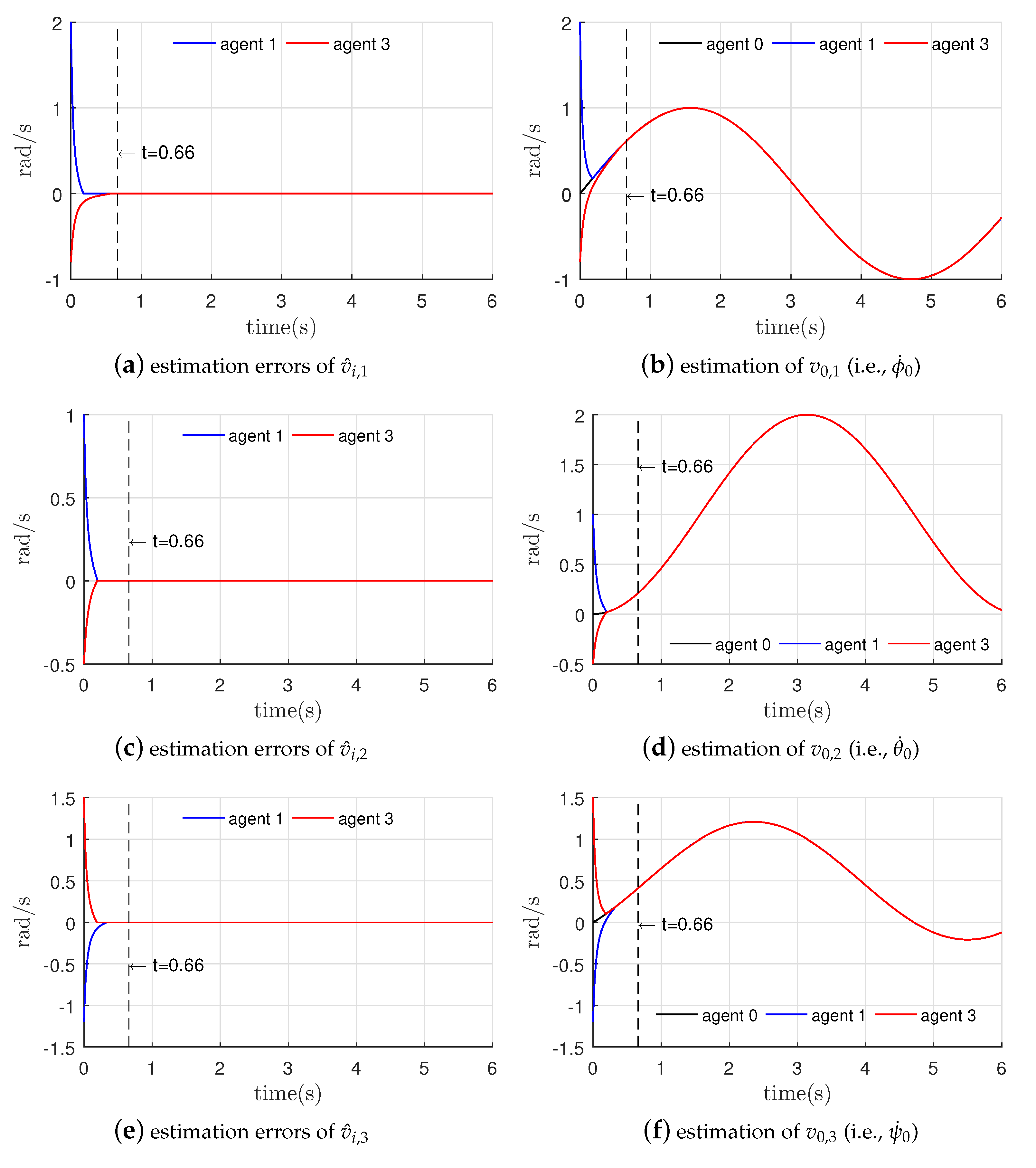
In
Figure 4a,c,e, it could be seen that estimation errors of the REDFTO converge to zero in a fixed-time. Therefore, the REDETOs for
,
could estimate velocity state of the virtual-leader exactly after
, which could be easily seen in
Figure 4b,d,f.
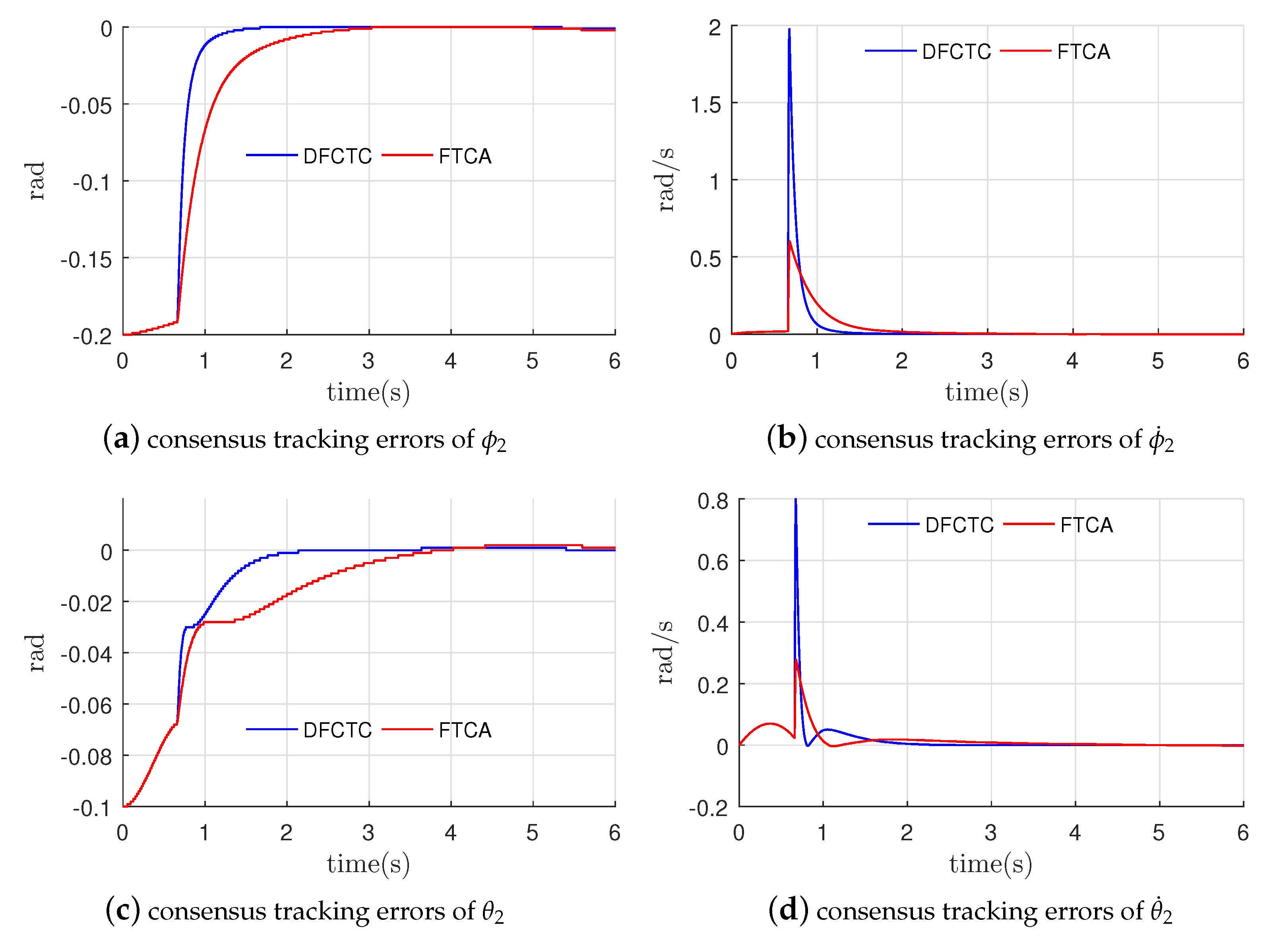
Note that, during the time interval
, the used control law is the LDC law expressed in the first line of (
55). When the time is greater than
, the used control law is the DFCTC expressed in the second line of (
55) (the blue lines) or the FTCA proposed in [
25] (the red lines). As illustrated in
Figure 5,
Figure 6,
Figure 7 and
Figure 8, when the proposed DFCTC is adopted, the attitude consensus tracking is achieved in a fixed-time. Obviously, convergence speed of the DFCTC is faster than that of the FTCA. The reason is that the settling-time of the DFCTC is independent of the initial conditions. However, settling-time of the FTCA is dependent of the initial conditions.
In
Figure 9, it is easily observed that the value of the control signal
is almost equal to the opposite value of the disturbance
after the time
. What this means is that the control signal could largely compensate the disturbance when the consensus tracking errors enter a small bounded set around the origin. Note that the overall disturbance
, which is expressed as
, consists of two parts: uncertainty
acting on the
i-th rigid-body and acceleration of the virtual-leader
.
,
,
are three components of
(i.e.,
), and
,
,
are three components of
(i.e.,
).
In
Figure 9, at the time instant
, the control signals are slightly larger. This is because the control law is switched from the LDC law to the DFCTC law at the time instant
.
5. Conclusions
The attitude consensus tracking problem has been investigated for a group of multiple rigid-bodies with time-varying uncertainty acting on each agent. The reference command profile has been seen as a virtual-leader, and a REDFTO used to estimate velocity state of the virtual-leader has been developed. Subsequently, a DFCTC law has been proposed. Fixed-time convergence of the tracking errors to a bounded region including the origin has been analytically proved. In the simulation section, a comparison case study confirms the effectiveness and superiority of the proposed control scheme.
However, there are some limitations with the proposed DFCTC law. As stated in Remark 5, estimation of the convergence time is more conservative. From the simulation results, when in the time interval , the DFCTC law is not used. These two limitations must be improved in the future work.


