1. Introduction
In recent years, with the construction of many large water conservancy projects, unidirectional flow pumping stations have found difficulty in meeting the needs of the project in practice, such as in large water transfer projects, both in irrigation water delivery and also to take into account the drainage in years of major flooding. Vertical axial-flow pumps have the characteristics of high flow and low head, and are widely used in large pumping stations. Vertical bi-directional flow axial pump units are gradually being used in the field of drainage and irrigation due to their compact structure and space-saving advantages. The combination application of a bi-directional flow channel and vertical pump has achieved great social and economic benefits. In recent years, vertical bi-directional flow axial pump station operation is often found cracked at the pump blade, sometimes even blade fracture, damaging equipment. Therefore, the structural strength of the vertical bi-directional flow axial pump blade and the stress distribution calculation and analysis are particularly significant.
In the study of pump unit performance, fluid–solid coupling is a quite effective tool for analyzing the flow field properties of fluids. Qin et al. [
1] used the sequential coupling method to study the strength of the impeller and guide vane of a large vertical shaft cross-flow pumping station in China under three different operating conditions. Zhang et al. [
2] performed the same calculation method on a submersible Axial-flow pump under multiple operating conditions and analyzed the stress and strain distribution patterns of rotor components under fluid forces, centrifugal forces, and gravity. Shi et al. [
3] analyzed the effect of fluid–solid coupling on pump head and efficiency through the joint solution of the internal flow field and the response of the structure of impeller of axial-flow pumps by bidirectional sequential fluid–solid coupling. Gao et al. [
4] analyzed the impeller stress characteristics when cavitation did not occur, when cavitation was incipient, and when cavitation was severe by the sequential fluid–solid coupling method.
Impeller is a rather significant component inside the pump unit, and the parameters of the impeller have a certain regulatory effect on the hydraulic performance of the pump unit. As a result, scholars have conducted a great deal of research on the flow field characteristics of impeller blades. Persch et al. [
5] studied and researched the highly unstable flow field characteristics in single-vane and two-vane pumps by supplementing the measured and simulated results to compare the pressure and flow undulation characteristics of the two pump types. Ju et al. [
6] conducted a comparative analysis of different shapes of vanes from the internal vortex structure and found that 2D and 3D forward-angle vanes have a better effect on pump hydraulic performance than conventional radial straight vanes, producing more intense fore-and-aft swirls and smaller axial and radial eddy currents in the vane channel and higher pump efficiency. Numerous studies have shown that the structural strength of the impeller has a direct impact on the safe and stable operation of the pump. The numerical simulation of the impellers studied is grouped by Chen et al. [
7], and different vane entrance angles are set, and it is found that the change in the vane inlet angle distribution has different effects on the pump performance, which is beneficial to the design of the vane centrifugal pump and its performance improvement. Zhang et al. [
8], He et al. [
9], and Pan et al. [
10] applied this method in axial-flow pump to compute the intensity of the impeller and found that the maximum value of stress appeared at the junction of the blade and the hub, the most evident deformation appeared at the entrance side of the blade near the rim, and the point where the stress is prominently concentrated was at the combination of the root of the blade and the hub. Liang et al. [
11] studied the blade stress distribution under different degrees of cavitation and found that with the occurrence of cavitation, the maximum equivalent force suffered by the impeller blade slowly reduces and the blade deformation increasingly decreases.
At present, relatively little research has been conducted on the strength of the impeller of vertical bi-directional flow channel axial pumps. This paper adopts model tests and numerical simulations, etc., takes a 3D solid modeling of a vertical axial-flow pump device as the research target, comprehensively analyzes the interior flow rate and stress field distribution of the axial-flow pump device, and a unidirectional fluid–solid coupling analysis is conducted for the distribution of stress field and deformation of the axial-flow pump blade under three operating conditions, which provides a basis for the design of the vertical axial-flow pump blade and makes reasonable recommendations for the stable operation of the axial-flow pumps.
2. Calculation Method
Fluid–solid coupling research explores various behaviors of solids that have been deformed under the effect of the flow and the interaction between the two [
12]. The effect of solid deformation on the flow domain is also a significant topic in this subject [
13]. The fluid–solid coupling fully reflects an interaction among two fields [
14]. The solid is changed under the load of the flow field; meanwhile, the distribution of the flow field also changes under the deformation and movement of the former. Therefore, fluid–solid coupling is an undoubtedly important means to effectively research the impeller flow field.
The internal flow of an axial pump is 3D viscous turbulence, which cannot be compressed and follows the equation of continuity and momentum equation of the fluid domains; the continuity equation is also known as the mass equation [
15].
This paper cites the RNG k-ε [
16] turbulence model for the derivation of the flow domain inside the pump during operation. RNG k-ε model can be well applied in a series of fluid calculations in pumping stations which are equipped with axial-flow pump [
17,
18,
19,
20]. The equation for k and the equation for ε are as follows.
In the formula, ; ; the constants take the values: , , , , β = 0.012.
2.1. Solids Control Equations
The conservation equations for the solid domain can be derived from Newton’s second law as follows.
2.2. Structural Dynamic Equations
When the axial-flow pump is in motion, the fluid which exists inside the pump applies load on the impeller, and it causes the impeller to produce response accordingly by Hamilton’s (Hamilton) principle; the structural dynamic equation [
21,
22,
23] is defined as follows:
The stress equation for the impeller structure calculation is as follows.
Calculation of the equivalent force based on the fourth strength theory combined with the
σ is obtained from the above equation.
2.3. Computational Model and Simulation Method
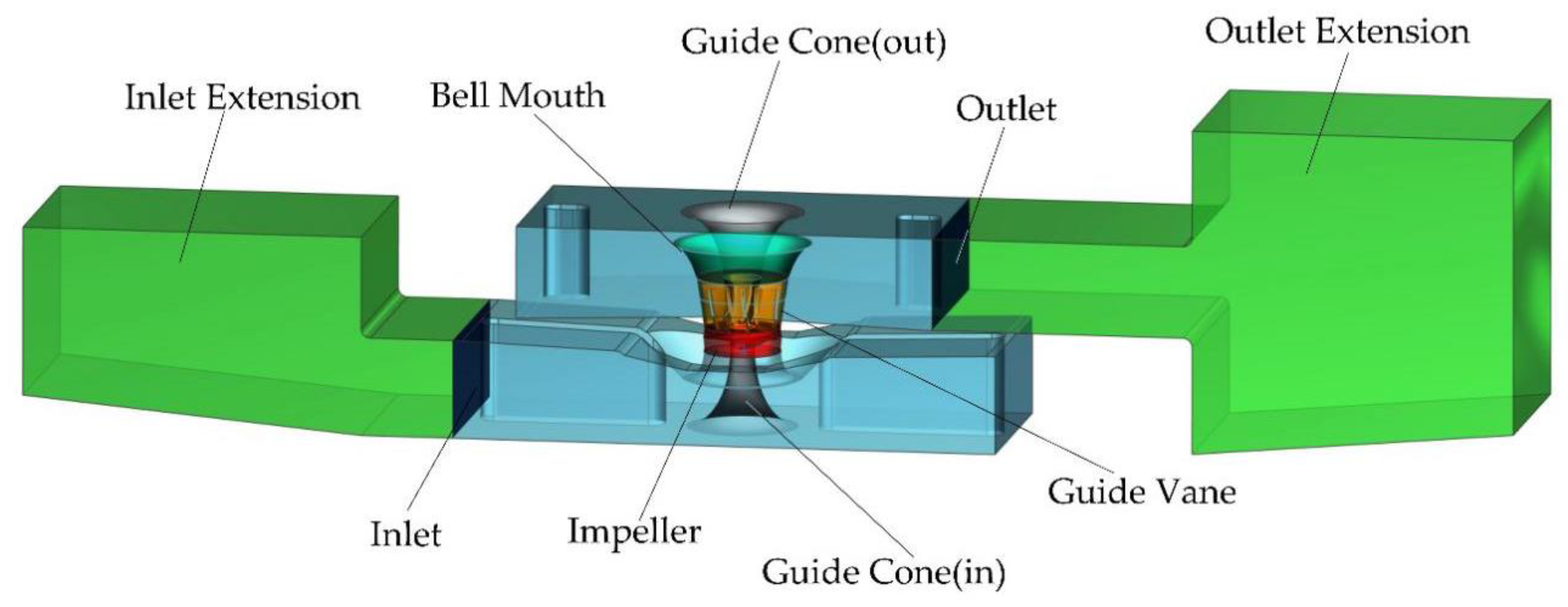
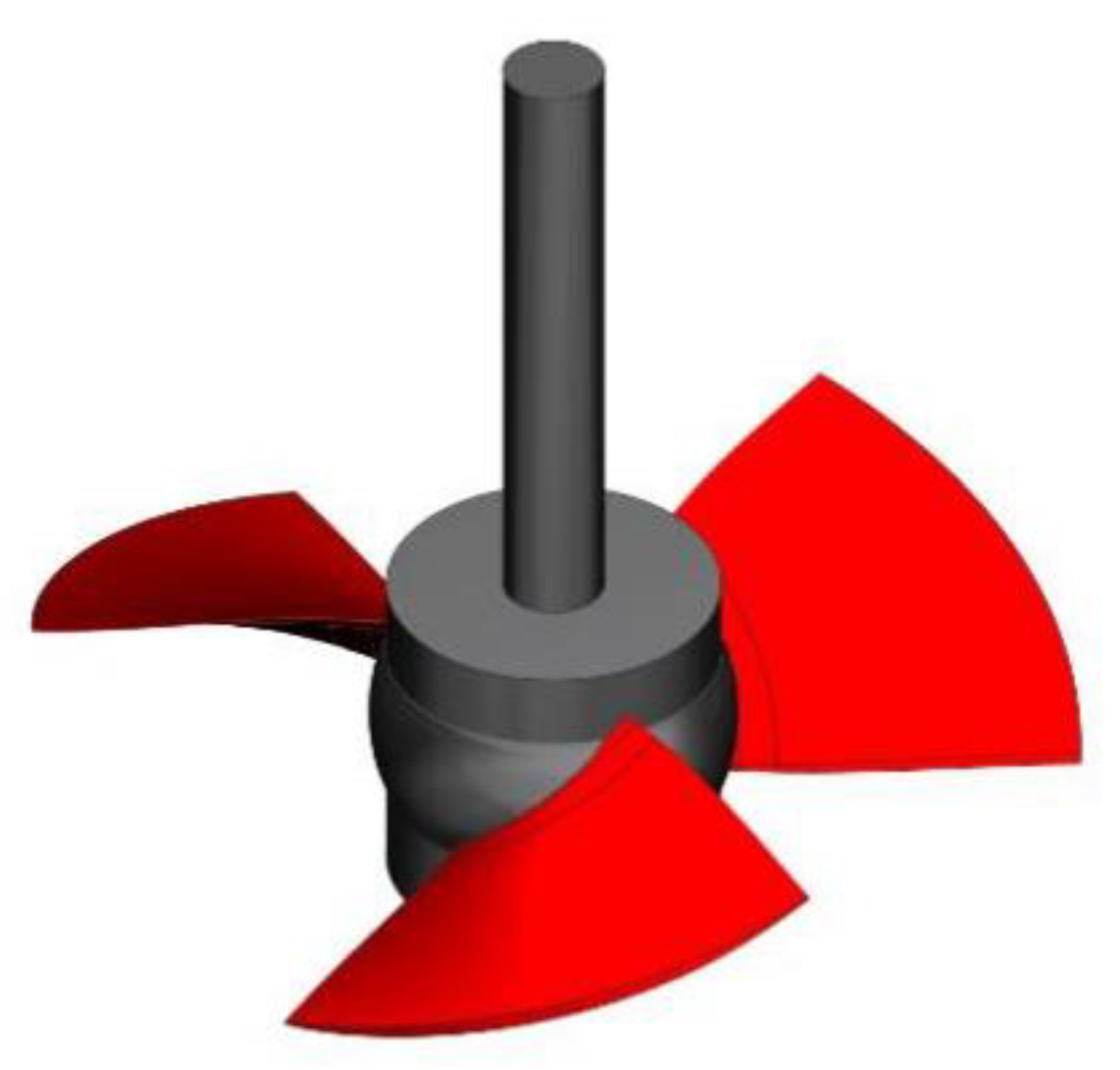
In this study, 2500ZLQ-20-3.0 vertical axial-flow pump is the researched target, the fluid domain includes the inlet and outlet section, impeller, guide vane, the basic parameters of the pump are flow rate = 20 m3/s head = 2.61 m, speed n = 150 r/min, number of vanes Z = 3, number of guide vane vanes = 5.
First, the 3D model of the axial pump impeller and the bi-directional flow channel was built in NX 9.0 as
Figure 1 and
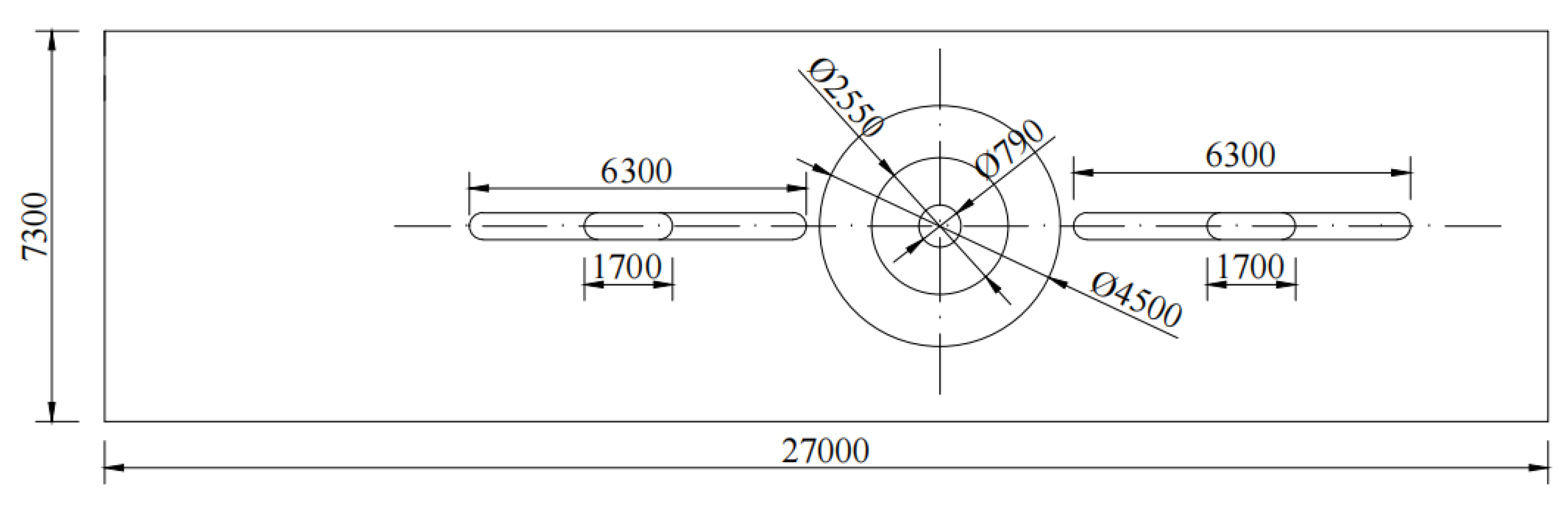
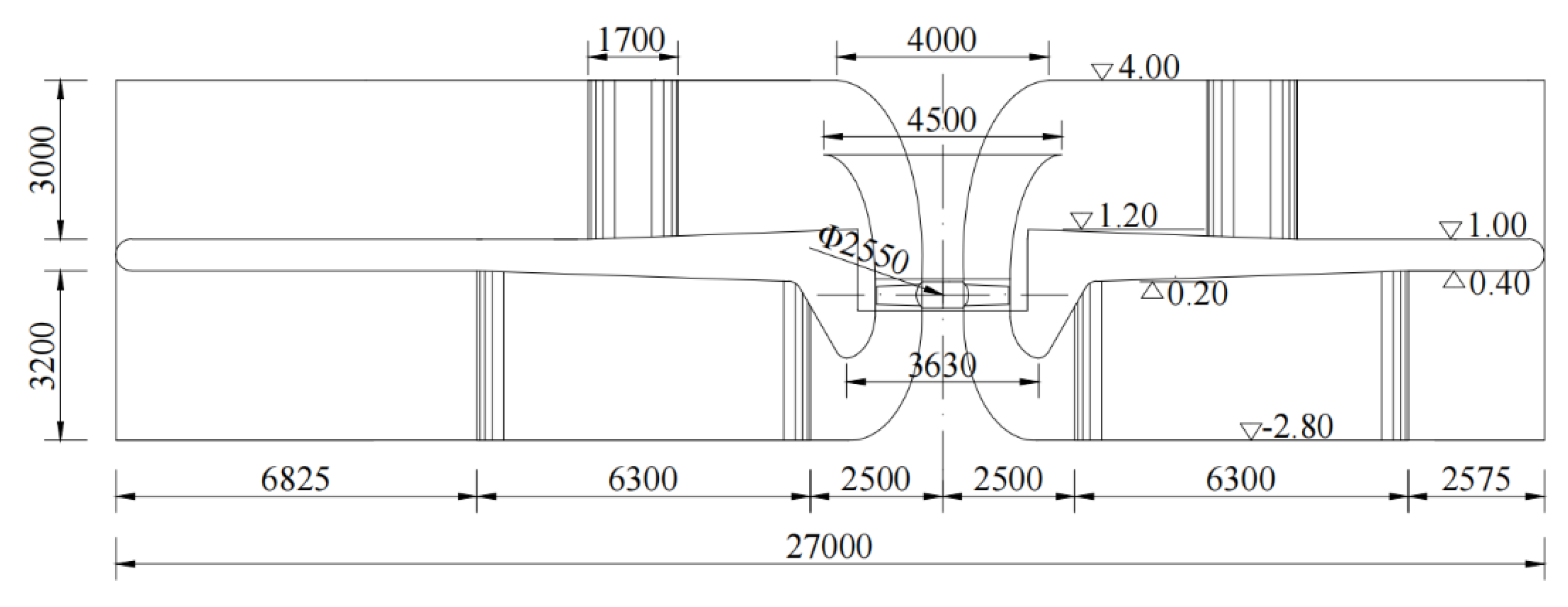
Figure 2 show. The exact dimensions of the model are shown in
Figure 3 and
Figure 4. According to the running conditions of the pump, its hydraulic and force characteristics are studied. The RNG k-ε turbulence model is applied in the software that called CFX to make numerical simulation of the 3D non-constant turbulence in the flow channel, and make validation of the external features to receive the eigenvalues of velocity, pressure, and other distributions of the flow field.
2.4. Grid Division
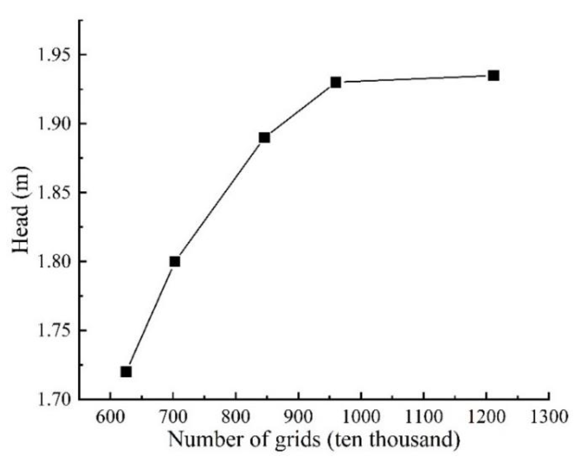
In this paper, the structured meshing of the full flow channel as well as the water column of the impeller and guide vane is used for the calculation of the fluid, using the meshing software ICEM. The design flow condition was selected to perform a grid independence analysis of the fluid domain of the pump unit, and the results are shown in
Figure 5. When the total number of grids is greater than 9.56 million, the relative error of the pump unit head change is less than 1%, taking into account the efficiency and accuracy of the calculation. In this paper, the number of grids in the fluid domain of the pump unit is set at 9.56 million.
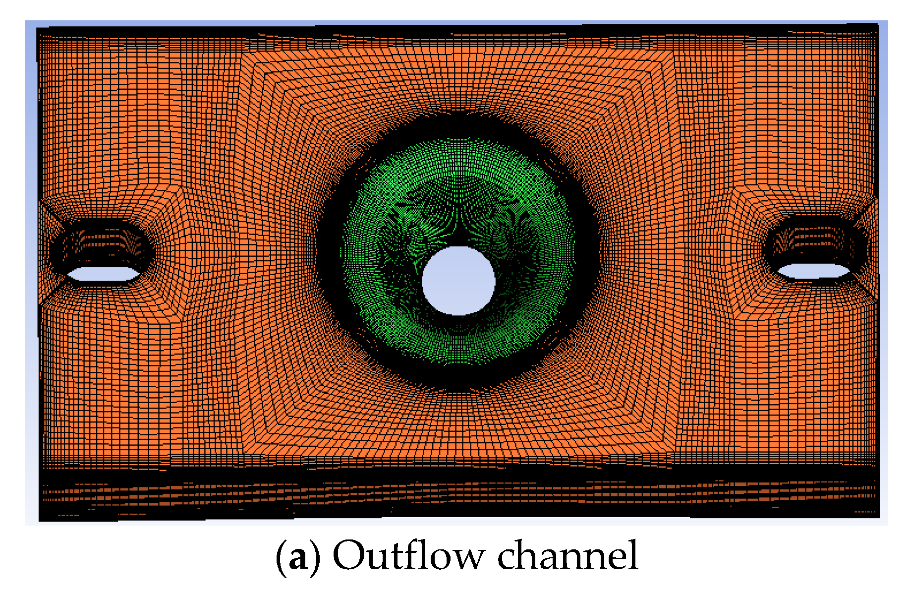
The meshing of the whole calculation area is shown in
Figure 6. For the impeller solid domain, ANSYS Workbench was used to unstructured mesh the impeller solids and encrypt the wall mesh for the solids.
The area of the fluid calculation includes the inlet channel and its extensions, the impeller, the guide vane, the outlet channel, and its extensions. The inlet of the inlet channel extension is the inlet boundary [
24] of the entire pump unit and the boundary is mass flow rate; the inlet flow rates are 10 m
3/s (small flow condition), 20 m
3/s (design condition), and 28 m
3/s (high flow condition), respectively, with a turbulence intensity of 5%. The outlet boundary is located at the outlet of the outflow channel extension, where the turbulent motion is in relative equilibrium and the flow state does not affect the flow field in the upstream direction. The outlet boundary is taken as average static pressure with a pressure setting of 1 atm. No-slip condition for viscous fluid is used on solid wall, the impeller surface and the hub surface as moving wall, the inlet channel and its extensions; the outlet channel and its extensions are set up as static wall (wall). The intersections set up in this paper are of two types; one is the dynamic and static intersection, set up between the impeller and the guide vane, the impeller and the inlet guide cone with frozen rotor. The other is the static intersection, set at the junction of the rest of the chunking grid with general connection. The accuracy of calculation is 1.0 × 10
−5.
2.5. External Characteristics Test
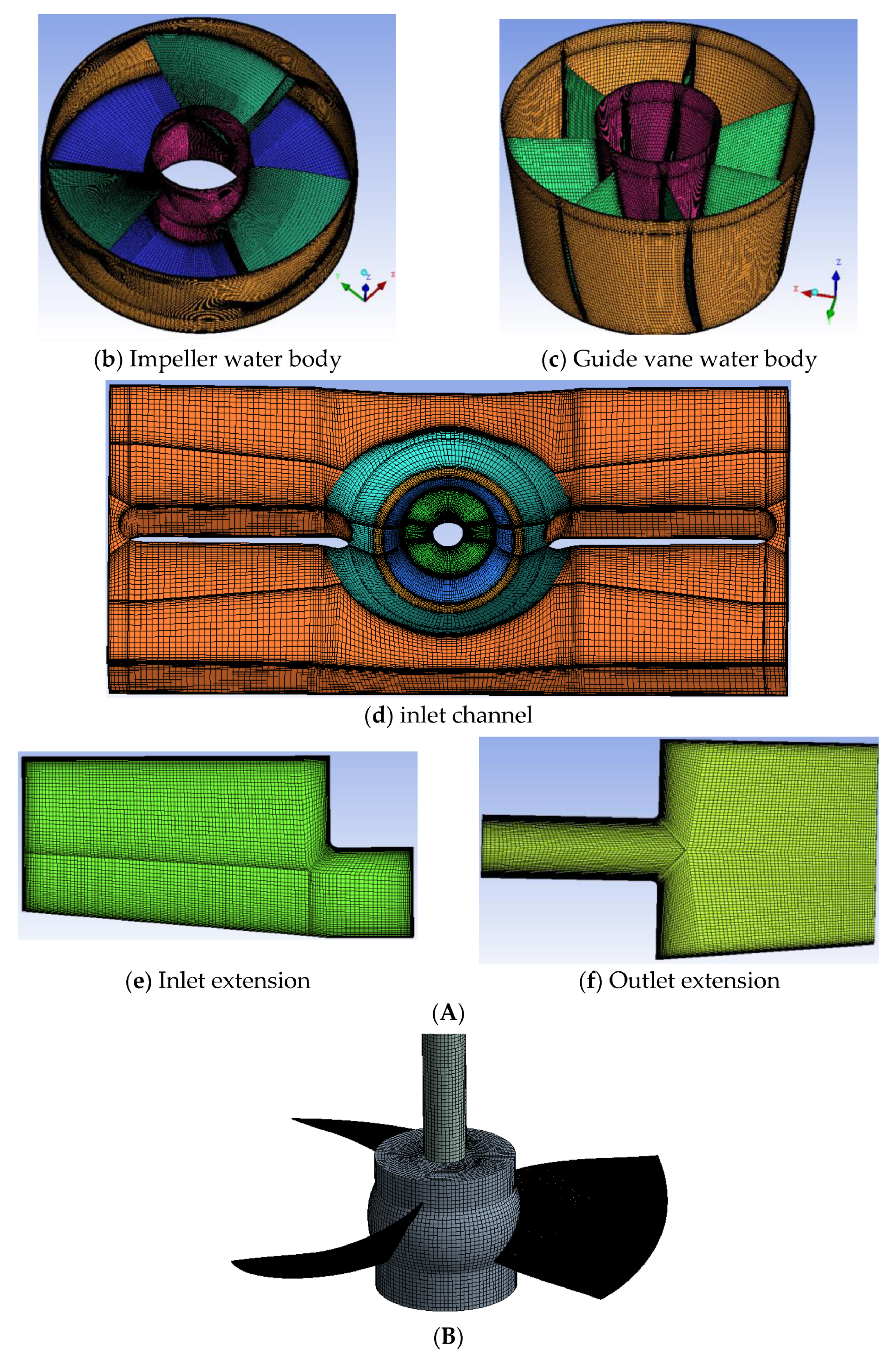
The model test bench of the pump device as shown in
Figure 7 was set up in the laboratory of the Engineering Hall of the College of Water Resources Science and Engineering of Yangzhou University. The whole test bench consists of inlet and outlet cistern, tested pump device, turbine flow meter, electromagnetic flow meter, booster pump, differential pressure meter, gate valve, etc. The pump unit test stand system is indicated in
Figure 7. The breadth of the model impeller for the test is 120 mm, the diameter of the prototype impeller is 2.50 m, and the similar ratio
λD is 20.83. Model pump device test speed is converted in light of the date received from prototype pump and model pump
nD value equal (i.e., equal head) for conversion, where
n is the impeller speed and
D is the impeller diameter, after a conversion model pump test speed of 3125 r/min.
The pump unit performance data measured by the test bench are converted in accordance with the mentioned method used to convert prototype pump performance in the SL140-2006 ‘Pump Model and Device Model Acceptance Test Regulations’. The conversion formula is.
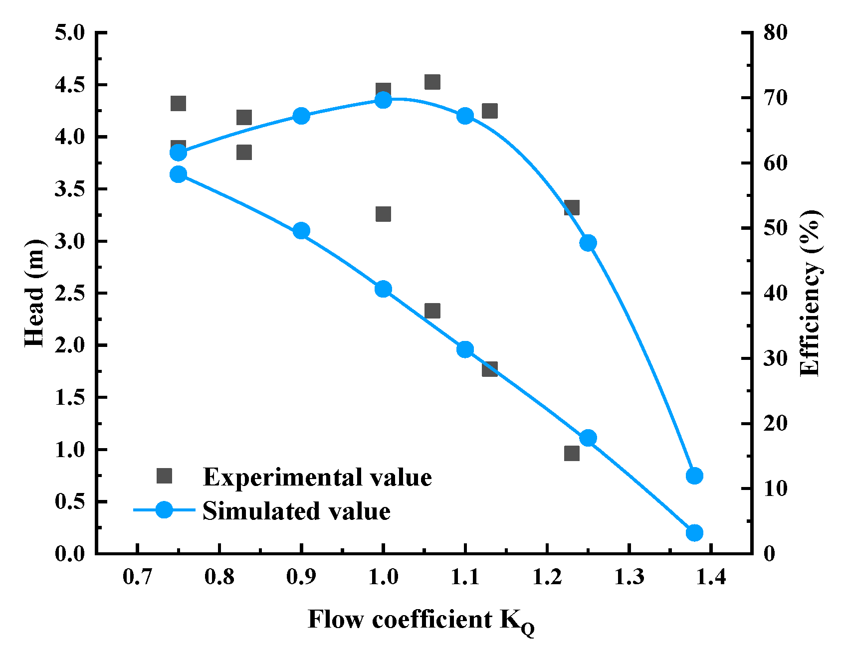
As shown in
Figure 8, by comparing the performance data of the prototype pump deduced by conversions and the performance curve of the device received by numerical simulation, the overall tendency is similar. The efficiency of the pumping unit gradually decreases with the increase in the flow rate; the head shows a trend of increasing and then decreasing with the increase in the flow rate, and the average error of the numerical simulation is within 5%. However, the distinction is more apparent when the flow coefficient
KQ < 1, and the values are alike with less error when
KQ > 1. The flow coefficient
KQ in the figure is the ratio of calculated flow rate to design flow rate. Often, the prototype pumping station is operated under high-flow conditions, and the head of the device is 0.01 m when the calculated flow reaches 1.4 times the design flow, so it is often adopted in operating conditions with high flow for its fluid calculation and analysis, whose data are highly trustworthy.
3. Calculation Results and Analysis
3.1. Vertical Axial-Flow Pump Flow Field Flow Velocity Distribution
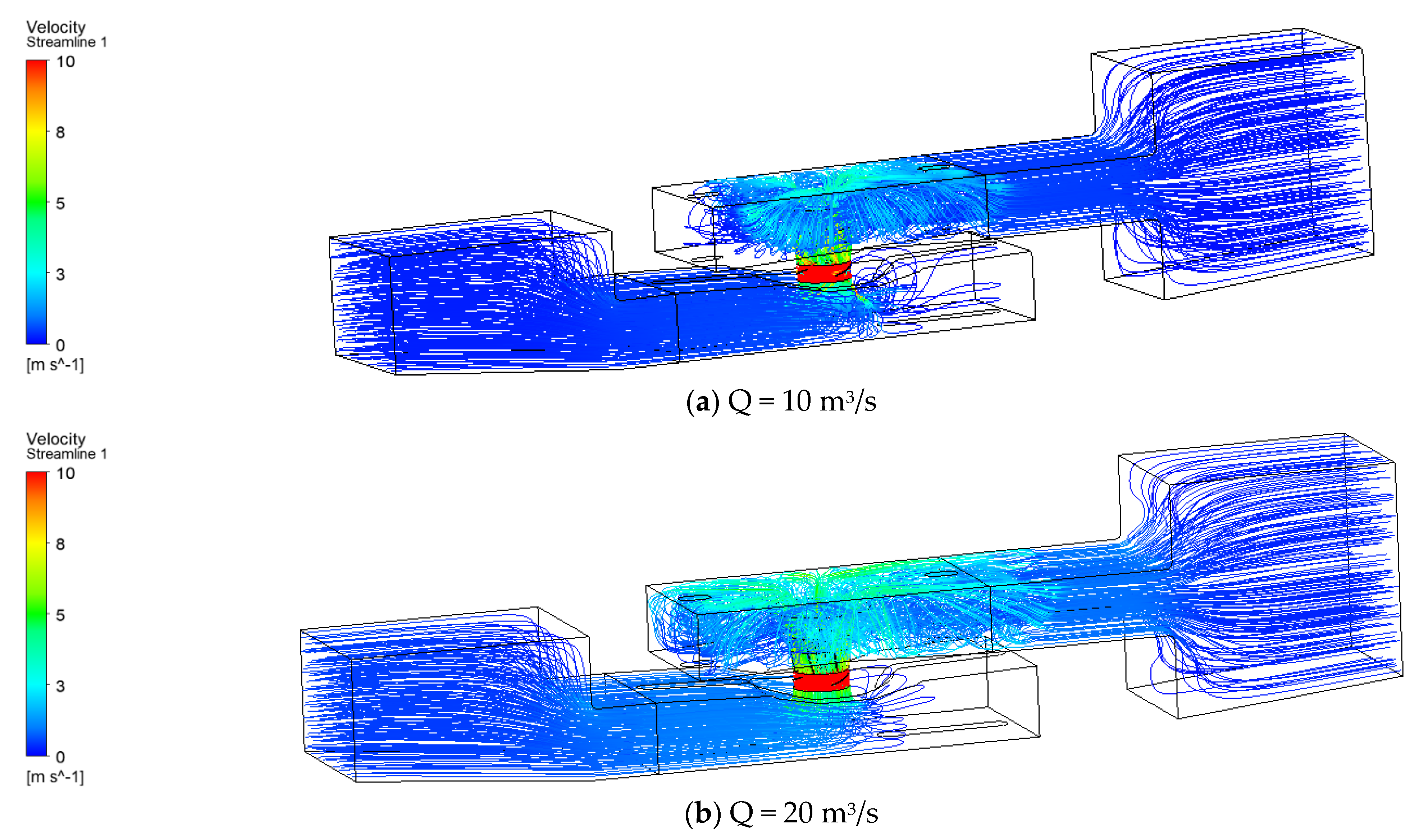
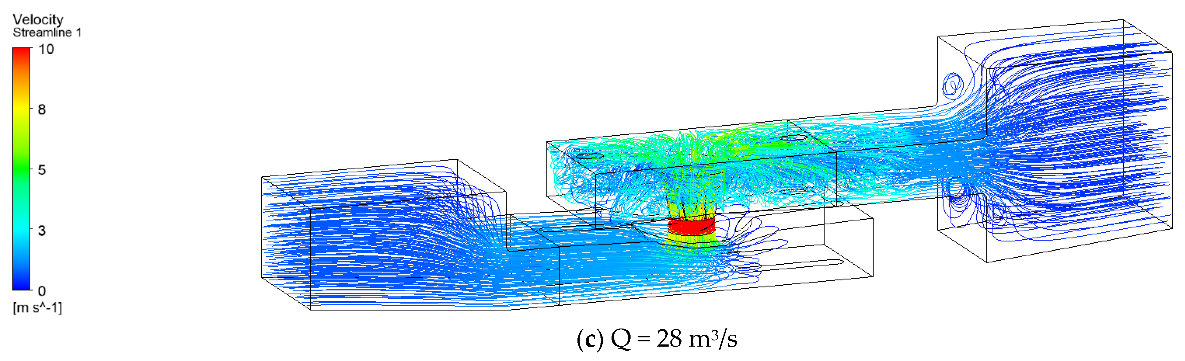
Figure 9 shows the flow diagrams of the full flow path of the axial-flow pump at 0.5, 1.0, and 1.4 times the design flow operating conditions.
From the flow diagram of the flow field, the flow velocity in the outflow channel gradually increases as the flow rate increases. The water flow in the inlet channel at different flow rates can be roughly divided into two parts. One is the stage where the water rushes into the intake channel and converges to the flapper pipe and the other is the adjustment stage. Most of the water flowing into the inlet channel enters the flapper pipe directly along the channel, with little water flow bypassing the sides and rear area into the flapper pipe. The water flow is constricted and adjusted in the inlet channel flapper pipe.
The water flow at different flow rates obtains energy in the impeller and then rotates into the guide vane body, which still has a certain amount of velocity ring after recovering part of the energy by the guide vane and spirals into the outflow channel. The water flow in the space formed by the horn pipe and the cone is rotating and spreading around, and the water flowing out of the space formed by the horn pipe and the cone is radially and sharply turning and spreading around, and the flow velocity is further reduced. Part of the water flows to the space behind the outflow channel and forms a large area of stagnant water here. The stagnant area in the outflow channel often produces a large range of backflow, and the area of backflow expands more and more as the flow increases. A portion of the water flow is blocked by the left- and the right-side walls as well as the stagnant area at the rear and is diverted to flow out; another part of the water flows directly in the direction of the outlet of the outflow channel in a spiral.
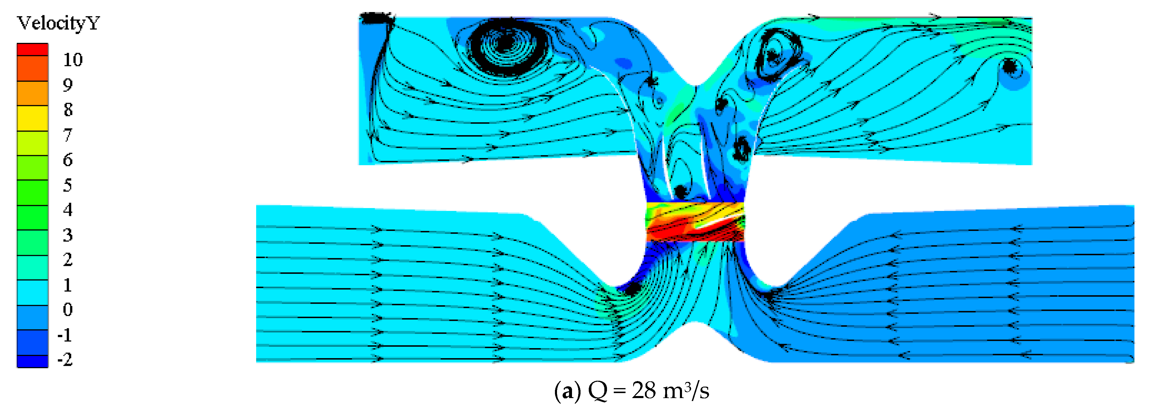
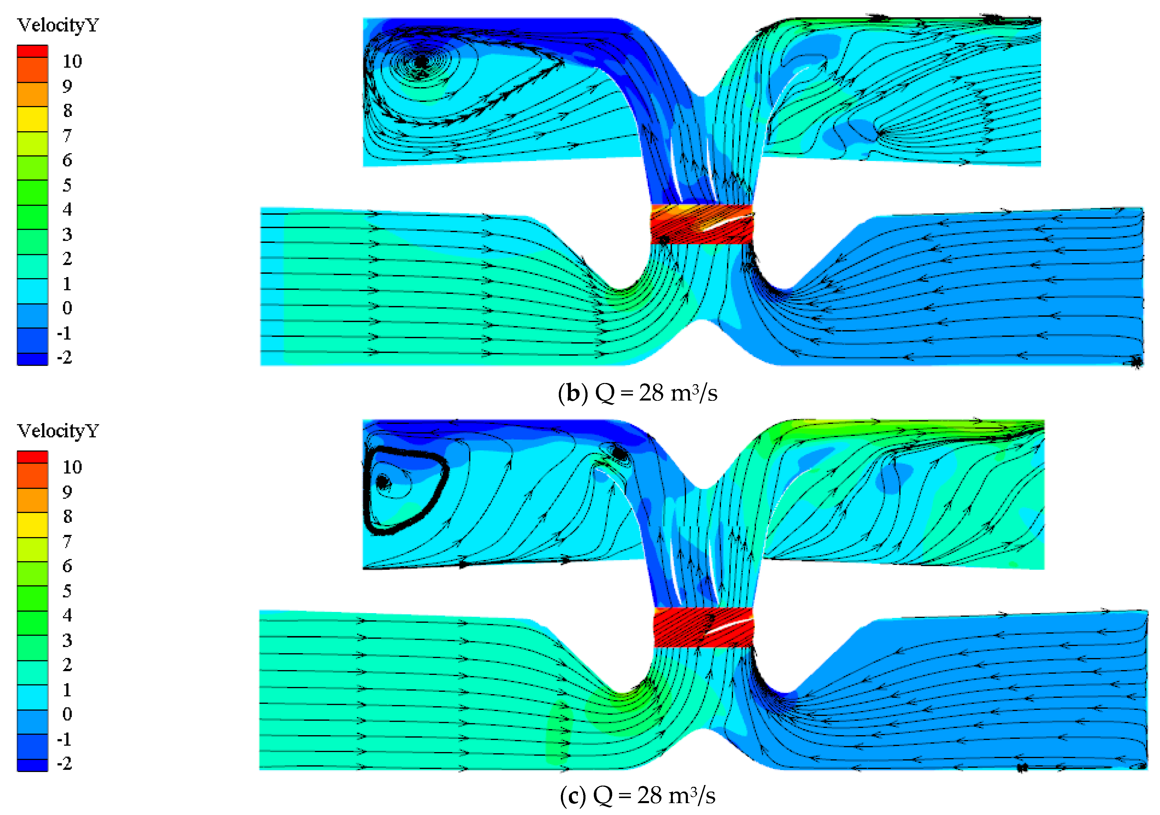
Figure 10 shows the flow diagrams of a cross-section of the full flow path of an axial pump at 0.5, 1.0, and 1.4 times the design flow rate.
As can be seen from the flow diagrams, under the low-flow conditions, the velocity of water in the flow runner is relatively low and a backflow zone is formed on the side of the stagnant water zone of the flow channel. Under the design flow condition, the range of the backflow within the stagnant water zone continues to expand, but the flow line is relatively flat, and a small vortex appears; then, the flow line readjusts to a uniform state. Under high-flow conditions, the backflow zone is further expanded, causing a large area of cyclonic roll in the flow channel.
3.2. Static Pressure Distribution of the Blade
The impeller is the core of the axial-flow pump; it is a significant working part of the axial-flow pump, and the blade is the main unit of the impeller. In many instances, cracks are raised by excessive stress concentrations at the structural transition between the blade and the hub, which affects the safe operation of the axial-flow pump. By calculating the three-dimensional flow field inside the vertical axial-flow pump device, the pressure situation suffered by the blade is obtained. The pressure distribution diagrams of blade surfaces are shown in
Figure 11,
Figure 12 and
Figure 13.
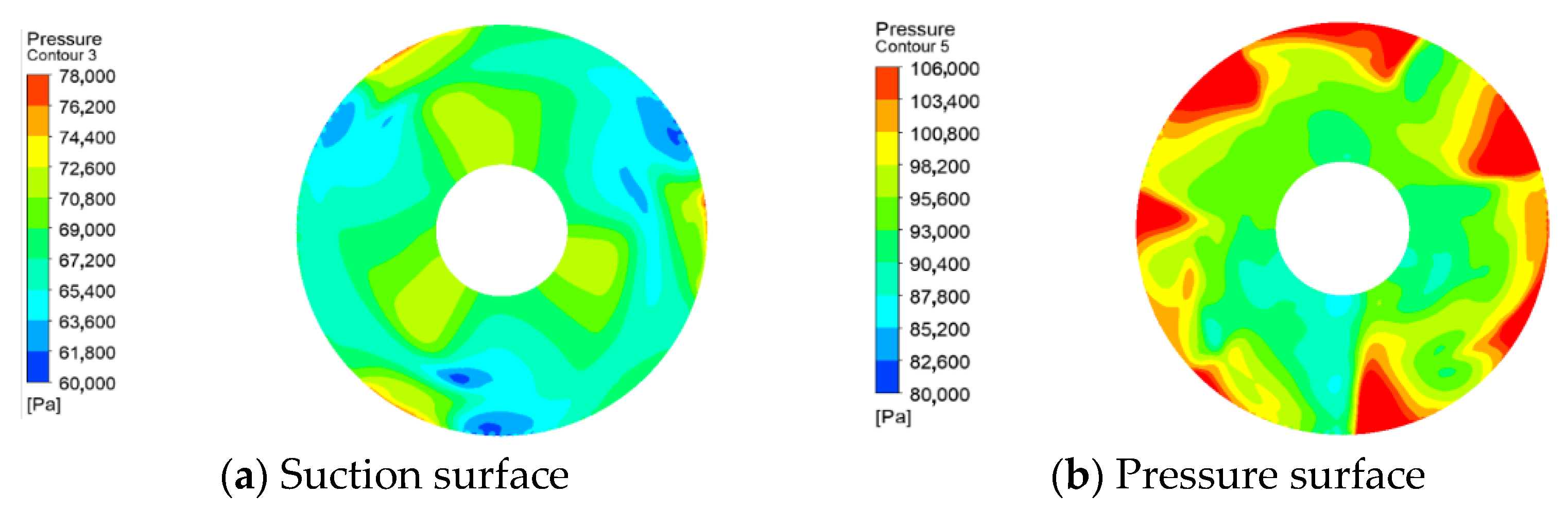
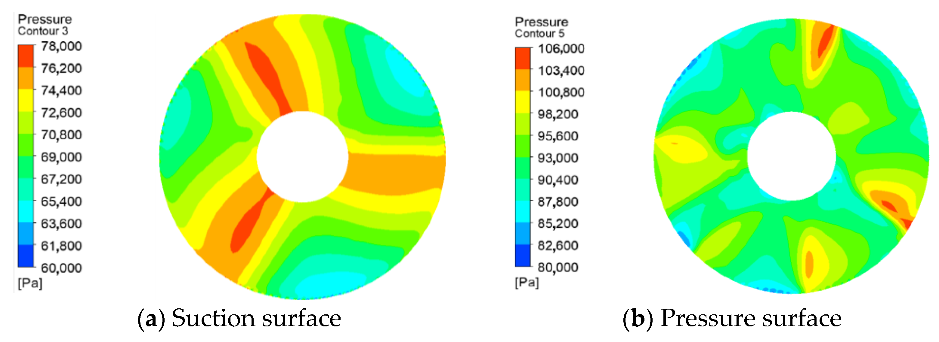
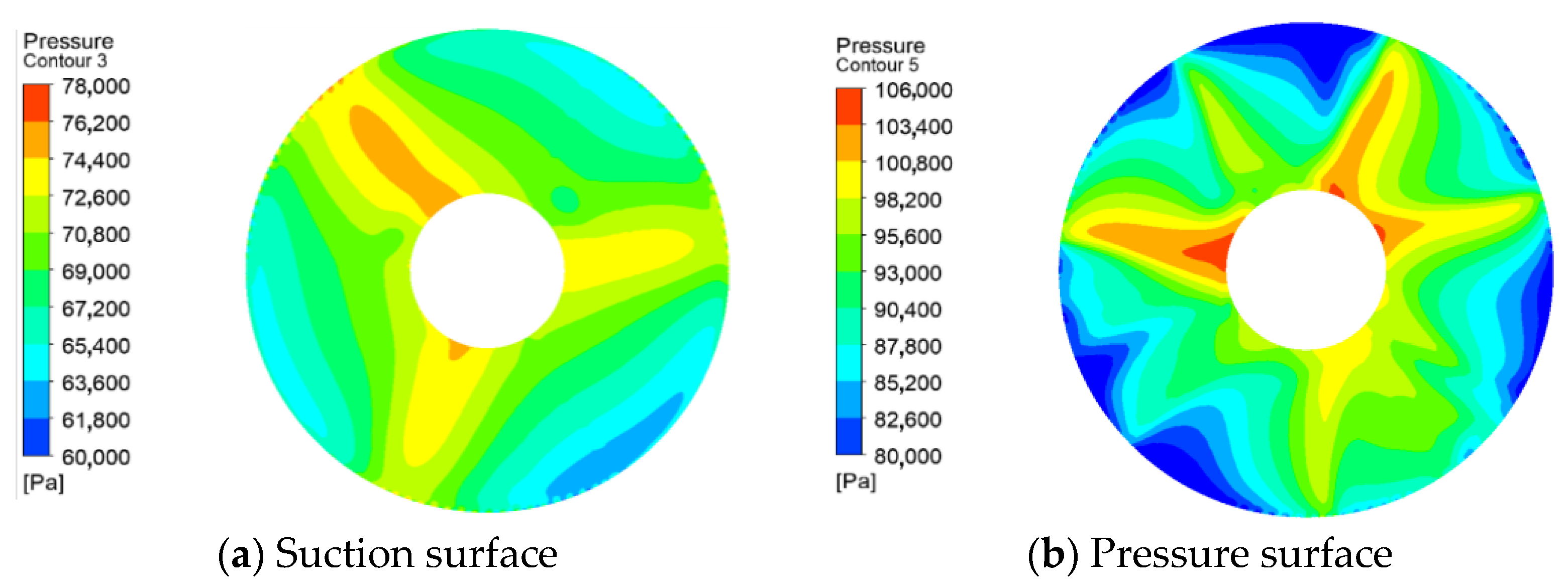
It can be discovered from the above figures that the pressure on the surface constantly varies periodically with the rotation of the impeller, whether on the suction or pressure surface, or under different flow operating conditions, and the static pressure distribution takes the shape of three petals, which coincides with the number of blades. In the nearby area of the rim at the inlet of the impeller, there appears a distinct low-pressure zone; the pressure in the vicinity of the blade is relatively high; with the increased flow, the range of the high-pressure area shows a trend of first increasing and then decreasing; and the pressure gradient distribution under the design conditions is more favorable to the water intake action.
The high-pressure area of the water body in the impeller is mainly in the vicinity of the blades. In the impeller outlet, the role of the guide vane begins to appear; as the water rises, the pressure at the hub gradually increases with the increased flow rate, while the pressure at the edge of the blade gradually decreases. There is a large pressure differential between the suction and pressure surfaces of the blades: the water flow under low-flow conditions is more easily lifted up to the guide vane, thus creating low pressure at the hub and high pressure at the rim, whereas under high-flow conditions the pressure distribution is exactly the opposite.
3.3. Stress Distribution of the Blade
When the water pump is in operation, the blade will rotate accordingly. During the rotation, the centrifugal force exits which can cause tension. The contact between the water and the blade creates friction force, and at the same time, the water pressure will then generate bending and torsional stresses. So, it can be seen that the blade force is quite complex. In order to study the distribution of the impeller equivalent force, this paper analyzes the blade equivalent force of a vertical axial-flow pump for three flow conditions based on the flow–solid coupling principle.
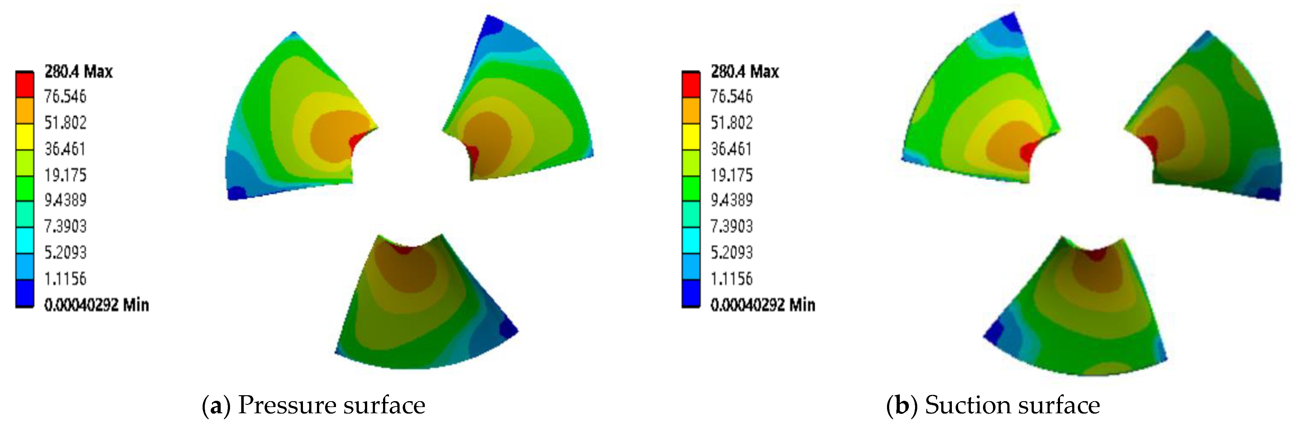
Figure 14 shows the equivalent force distribution of axial pump blade surfaces (suction and pressure surface) under 0.5 times the design flow condition. Under the small flow condition, the equivalent stress distribution spreads outward from the central point of concentrated stress at the entrance of the water flow, and the stress at the center position of the blade root to the middle part of the whole blade is relatively high, and the stress peak value is 280.4 MPa. The value of the equivalent force on the suction surface is slightly smaller compared to the pressure surface, while the stress value of the whole blade at the root and at the edge of the blade varies greatly.
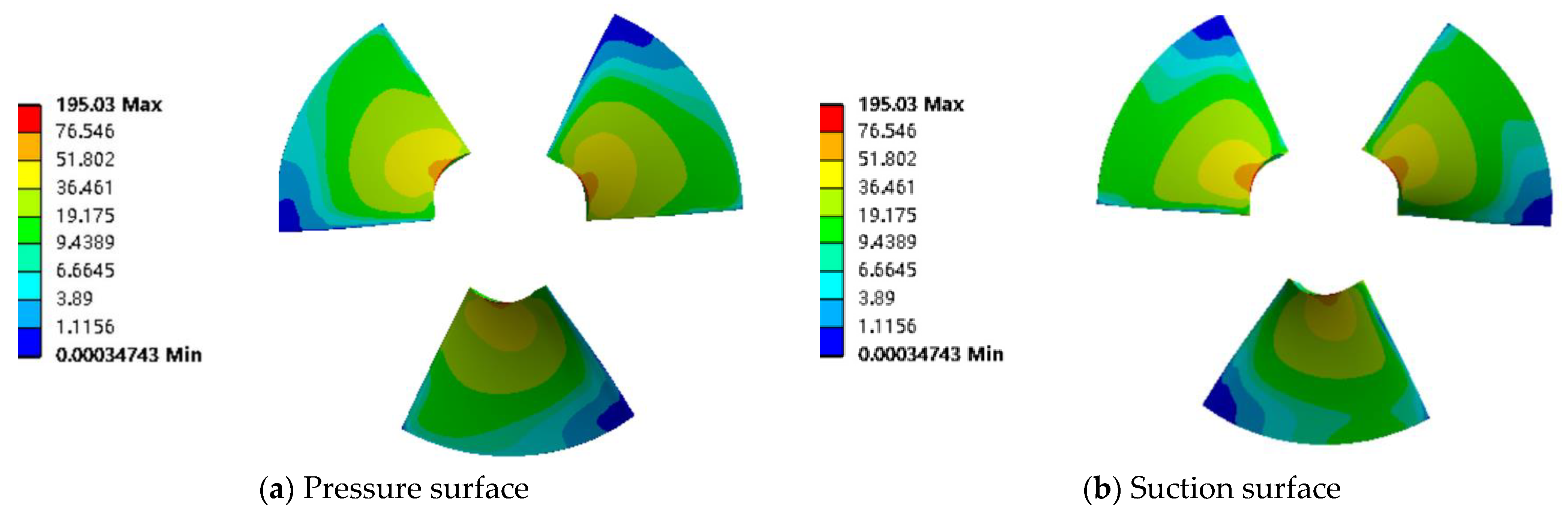
Figure 15 shows the equivalent force distribution of the suction surface and pressure surface of the axial-flow pump blade under the design flow condition. Under this operating condition, the blade equivalent stress concentration point is located in the middle of the blade root; its maximum stress value is 195.03 MPa. The stress distribution tends to decrease in all directions, and the stress value transitions more gently in the diffusion process suction surface, and pressure surface stress distribution law is basically the same; the difference between the stress value at the root and edge of the entire blade is small, and the blade by the stress is more uniform.
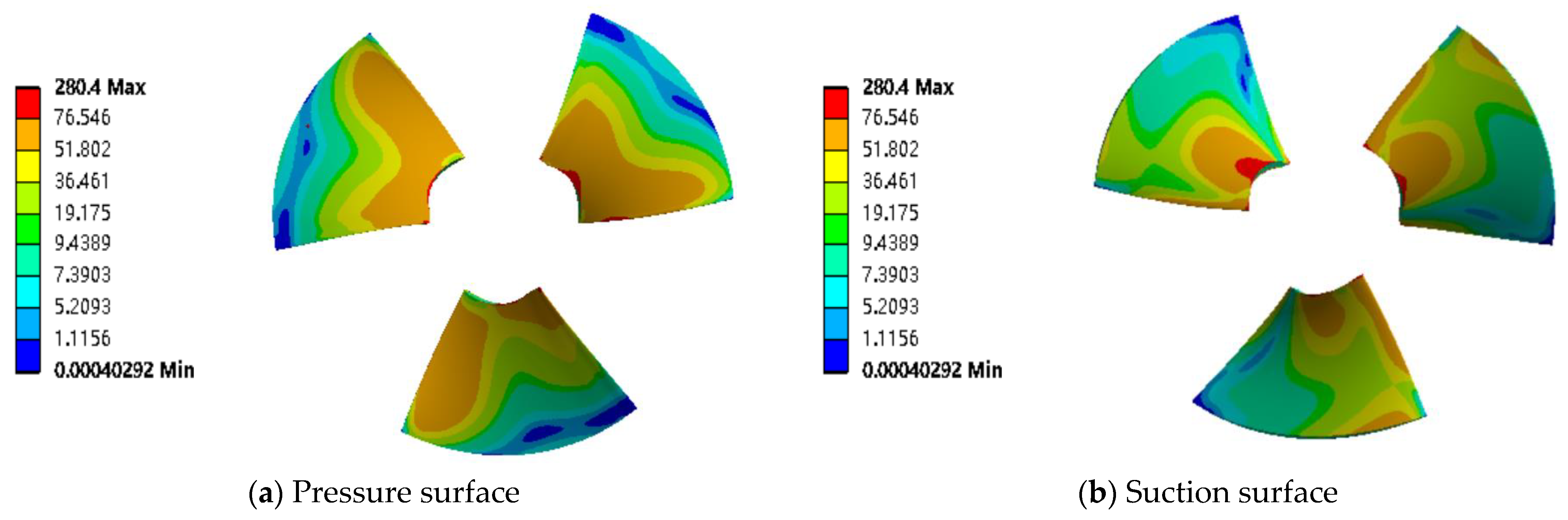
Figure 16 shows the equivalent force distribution of the suction surface and pressure surface of the axial-flow pump blade under 1.4 times the design flow condition. The water flow energy is stronger under the large flow conditions; the force exerted on the blade is more obvious. The thinner the thickness of the blade, the greater the pressure surface equivalent force value with the stress peak value at 62.6 MPa, while the suction surface stress value by the thickness of the influence is not large. Overall, the stress distribution of the blade suction surface and pressure surface shows decreasing tendency from the root to the outer edge along the radial. The stress value of the suction surface relative to the pressure one is small, but on the suction surface, the difference between the peak and trough values of stress is larger.
As can be seen from
Figure 14,
Figure 15 and
Figure 16, under the three working conditions, the peak values of the equivalent force are all occurring in the vicinity of the blade hub on the pressure surface of the blade, that is, the root of the blade on the water inlet side. The interface of blade and hub is a free surface, so the stress of the interface is not considered. There are more obvious stress concentration phenomena occurring on both surfaces of the blade near the hub. The stress distribution of the whole blade has a tendency to disperse outwards from the stress central point, which is at the location at which occurs the stress peak value near the hub on the water inlet, which is gradually decreasing stress outward; the rim of the blade of the water outlet side is where the stress is at its smallest. Under the same working condition, the difference between the stress value of the suction and pressure surface is not large and the law of the equivalent stress distribution is basically the same.
3.4. Deformation Analysis of the Blade
The results of the fluid–solid coupling revealed a slight deformation of the impeller blade,
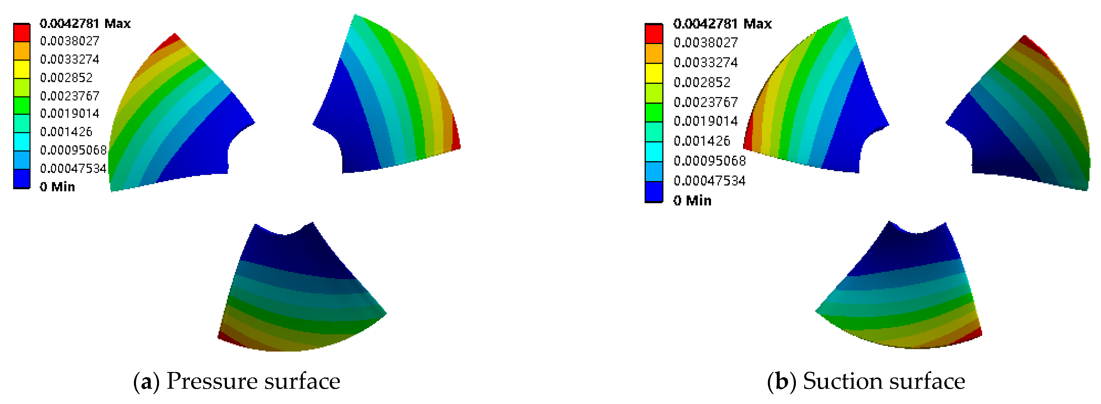
Figure 17 shows the deformation of the axial-flow pump impeller at 0.5 times the design flow condition. Under small-flow conditions, the deformation law of the suction surface and pressure surface of the blade are almost the same; the deformation peak is 4 mm, which occurs where the water inlet rim and outer edge intersect. The degree of the blade deformation decreases along the rim towards the hub, that is, the deformation condition becomes progressively better. There is no deformation of the blade at the hub.
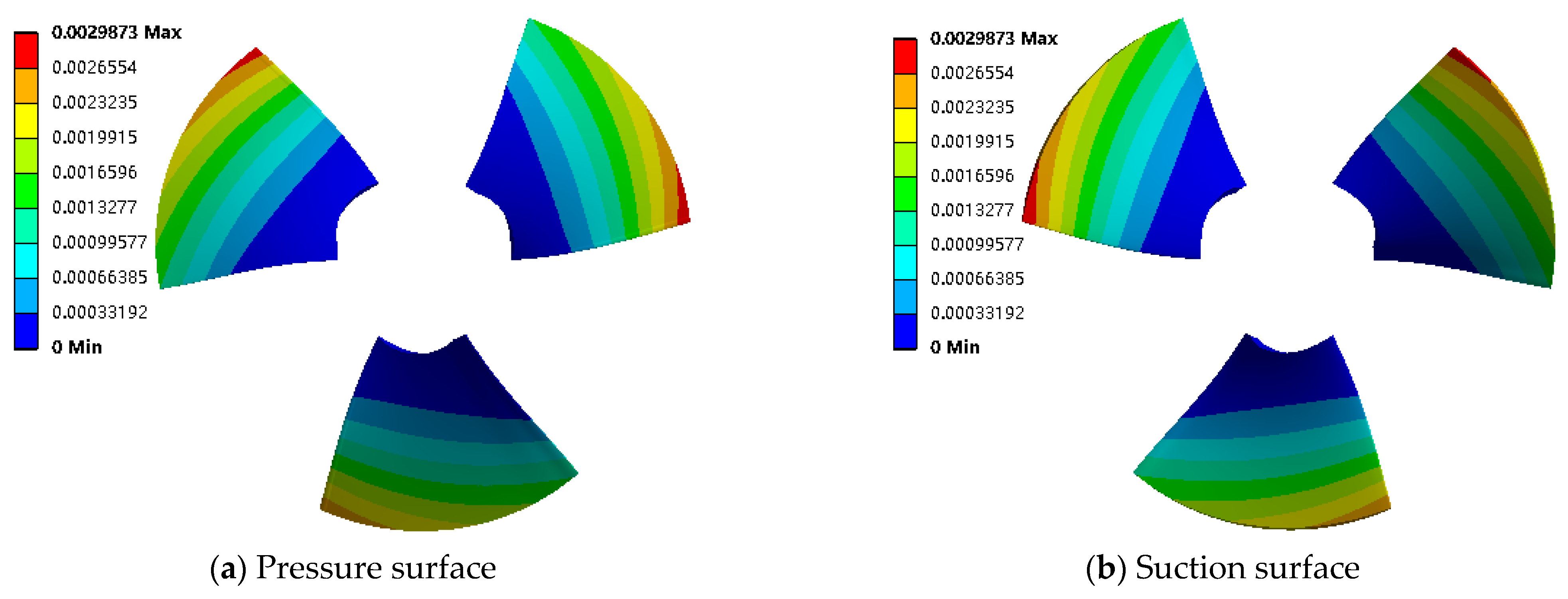
Figure 18 shows the deformation of the axial-flow pump blade under the design flow condition. The suction surface and pressure surface are basically similar in deformation position, the blade in the stress value is smaller at the outer edge of the deformation which is more serious, the maximum deformation is 2 mm, the deformation is smaller in the area closer to the hub, and the deformation value at the hub is 0.
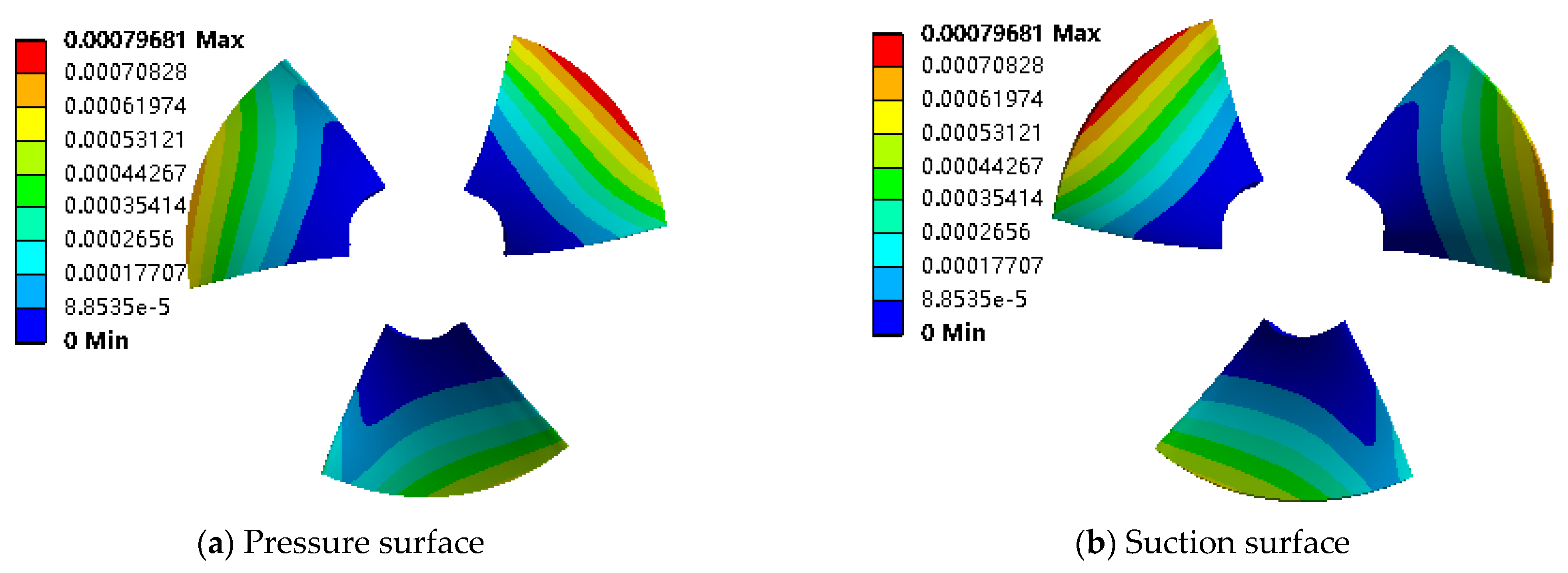
Figure 19 shows the deformation condition of the impeller of the axial-flow pump at 1.4 times the design flow rate. Under high-flow conditions, the area of the blade deformation region is relatively large, and the maximum deformation is 0.7 mm. The deformation law of the suction surface is similar to the pressure surface. The blade is deformed near the center of the outer edge and the deformation gradually decreases from the rim to the hub, with no deformation near the hub.
As can be seen from
Figure 17,
Figure 18 and
Figure 19, the most distinctive deformation of the blade mostly occurs at the outer edge of the inlet side of impeller. There is a gradual decrease in deformation from the edge to the hub, with no deformation occurring near the hub. The position of the greatest degree of deformation of the pressure surface and the suction surface is basically the same, and the size of the deformation is basically the same. Under the design working condition, the value of deformation will not be large, and the area where the deformation occurs will not be too large, which is conducive to making the blade maintain the original geometric parameters and ensuring the operation efficiency of the pump.
3.5. Comparative Analysis of Stress Characteristics
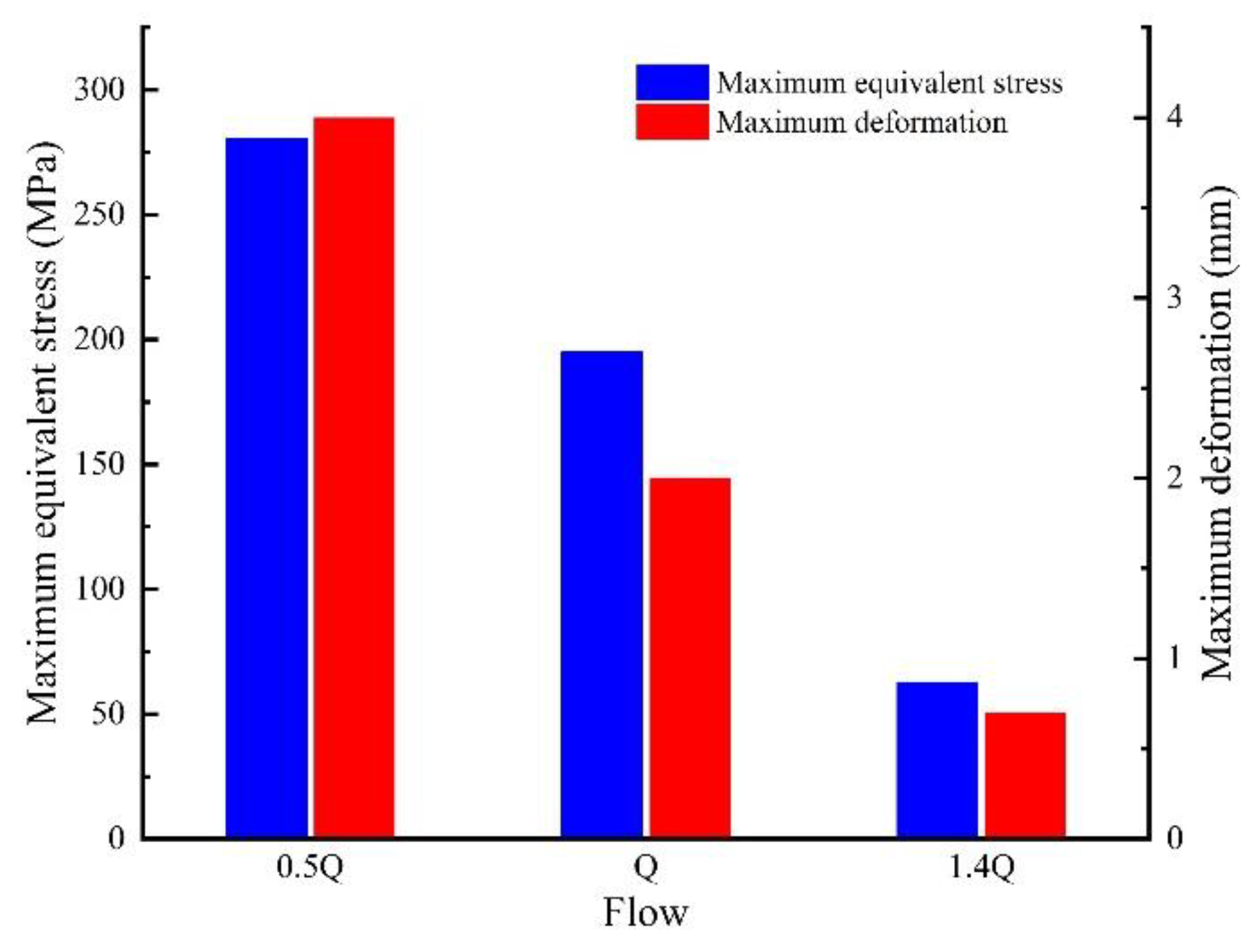
The maximum equivalent stress and maximum deformation of the blade under different working conditions are listed below.
As shown in
Table 1 and
Figure 20, the stress on the impeller blades varies significantly with the flow rate in the vertical bi-directional flow channel axial pump installations. With the increase in flow, the maximum equivalent stress and deformation progressively reduced. The shape characteristics of the impeller lead to a gradual increase in the equivalent force on the blade from the rim to the hub direction, with the maximum stress area appearing near the hub. As the flow rate increases, the maximum deformation of the blade shows a decreasing trend, and the range of obvious deformation in the blade increases with the flow rate.
The thickness of blades in the vertical bi-directional flow channel axial pump plays a dominant role in the amount of deformation of the blades, with the greatest thickness having the least amount of deformation near the root of the blades. Under the design working condition, the value of deformation will not be large, and the area where the deformation occurs will not be too large, which is conducive to making the blade maintain the original geometric parameters and ensuring the operation efficiency of the pump. The centrifugal force of the impeller is one of causes of the phenomenon of stress concentration at the root of the blade, and the complicated hydrodynamic operating environment is another significant reason for it. The combined effect of the two causes the blade to break. It has high probability to cause fatigue fraction. In engineering practice, the impeller generates cracks in the location of the blade root in most cases, which verifies the findings of this paper. There is only a fairly small gap between the blades and the pump casing; if the deformation of blade is too large, it will cause friction between the blade and the pump casing, affecting the normal work of the pump. In the design of an axial-flow pump impeller, the stress concentration near the root of the blades and the deformation at the rim of the blades should be fully considered; only by ensuring that both of these are within the permitted limits can the safe and stable operation of the impeller be guaranteed.
4. Conclusions
This paper presents a numerical simulation study of a vertical bi-directional flow channel axial pumping unit based on the continuity equation, the N-S equation and the RNG k-ε turbulence model, using a unidirectional fluid–structure coupling approach.
The blade stress characteristics of an axial-flow pump are analyzed in relation to the equivalent force distribution and deformation of the impeller blades in this study. This study can provide a theoretical reference for the optimization of the design of axial-flow pump vanes in order to prevent the fatigue fracture of the vanes that occurs more often during the operation of axial-flow pumps. The conclusions of this study are as follows.
- (1)
In the pressure distribution of the flow field of the axial-flow pump, a clear low-pressure area appears in the area near the edge of the impeller inlet, the pressure near the blades is relatively high, and as the flow rate increases, the high pressure area shows a trend of first increasing and then decreasing.
- (2)
Stress concentrations occur at the centre of the blade root–hub connection, with the maximum stress value at the stress concentration decreasing as the flow rate increases.
- (3)
The blade will be deformed in millimetres under stress, the maximum deformation is mainly distributed in the outer edge of the blade, and the closer to the hub, the smaller the deformation. As the flow rate increases, the blade deformation decreases.
For vertical bi-directional axial pumps, the conditions of the design flow conditions are more favorable for the safe and stable operation of the impeller blades.


