Reliability Assessment Method Based on Condition Information by Using Improved Proportional Covariate Model

Abstract

If sufficient historical failure life data exist, the failure distribution of the system can be estimated to identify the system initial hazard function. The conventional proportional covariate model (PCM) can reveal the dynamic relationship between the response covariates and the system hazard rate. The system hazard rate function can be constantly updated by the response covariates through the basic covariate function (BCF). Under the circumstances of sparse or zero failure data, the key point of the PCM reliability assessment method is to determine the proportional factor between covariates and the hazard rate for getting BCF. Being devoid of experiments or abundant experience of the experts, it is very hard to determine the proportional factor accurately. In this paper, an improved PCM (IPCM) is put forward based on the logistic regression model (LRM). The salient features reflecting the equipment degradation process are extracted from the existing monitoring signals, which are considered as the input of the LRM. The equipment state data defined by the failure threshold are considered as the output of the LRM. The initial reliability can be first estimated by LRM. Combined with the responding covariates, the initial hazard function can be calculated. Then, it can be incorporated into conventional PCM to implement the reliability estimation process on other equipment. The conventional PCM and the IPCM methods are respectively applied to aero-engine rotor bearing reliability assessment. The comparative results show that the assessing accuracy of IPCM is superior to the conventional PCM for small failure sample. It provides a new method for reliability estimation under sparse or zero failure data conditions.

1. Introduction

It is an important research issue how to guarantee the safety and reliability of a complex electromechanical system during its running process [1]. It is of great significance to prevent a major or catastrophic accident if the equipment failure can be estimated or predicted accurately in advance, which mainly depends on the reliability assessment techniques.

In general, the frequently used reliability assessment methods can be classified into two major categories: The traditional reliability analysis methods bases on large sample size failure life data and reliability analysis methods based on the performance degradation data. The former is required to obtain sufficient failure life data through reliability tests and then to acquire the equipment reliability index by using classical mathematical statistics. It lacks an individual characteristics description of the device itself [2]. The latter is required to acquire some professional background knowledge to evaluate the equipment degradation path or probability distribution function of the state features [3,4].

Due to the diversity, complexity, and randomness of the system parameters, loads, and environment, the mechanical system reliability is difficult to describe by using strict mathematical models. Too much simplification will influence the authenticity and credibility of the reliability models [5]. In view of the above problems, some researchers have begun to recognize the importance of the system operational condition information. Zio pointed out that the accuracy and reasonableness of reliability models will be improved if the operational condition information can be considered [6]. Li et al. [7] proposed a self-data-driven RUL prediction method for wind turbines considering continuously varying speeds by its own condition monitoring data without depending on failure event data. Yan et al. [8] investigated the degradation modeling and RUL prediction for dependent competing failure processes. The degradation models for both soft and hard failure processes are formulated, and the offline estimation and online update of parameters are jointly addressed. Chen et al. [9] proposed a new reliability assessment approach to cutting tools based on logistic regression model (LRM) by using vibration signals.

Proportional hazard model (PHM) was first proposed by scholar Cox to describe the system hazard risk with different joint covariates [10]. It has been widely used in life sciences, economics, electronic engineering, and preventive maintenance decisions [11,12]. In PHM, the baseline hazard function is established based on historical failure data, while the covariate function is established based on covariate data. If the covariates were replaced by the salient features extracted from the multi-resource conditional signals (vibration, force, torque, temperature, acoustic emission, etc.), the equipment conditional monitoring information can be introduced into PHM for reliability assessment and failure analysis [13]. Based on PHM model, the Center for Maintenance Optimization and Reliability Engineering (C-MORE) of the University of Toronto has developed the PHM’s algorithm and improved the CBM software (EXAKT), which has been applied to optimize the equipment operation strategy and maintenance costs [14]. In [15], the root mean square and peak index extracted from the vibration signals are severed as covariates of PHM to analyze the cutting tool reliability.

In PHM, a large number of failure data are needed to estimate the baseline hazard function and the weight parameters by Maximum Likelihood Estimation (MLE). The requirement limits the application effectiveness of PHM significantly when failure data are insufficient. Furthermore, the baseline hazard function is usually considered a constant function when the covariates are zeros. The hazard rate will change with the covariate of the system, i.e., the covariate is the explanatory variable and the hazard rate is the response variable. Actually, during the failure analysis process of an asset based on conditional monitoring data, the response covariates are extracted and applied to indicate the degree of equipment degradation. Under the circumstance, the covariates are response variables, and the hazard rate becomes the explanatory variable. Therefore, PHM is not appropriate for this condition.

To solve the above problems, Sun has proposed a new model named as proportional covariate model (PCM) to describe the hazard rate of a mechanical system [16]. PCM reveals the dynamic relationship between the response covariates and the system hazard rate. The system hazard rate function can be constantly updated by the response covariates through the basic covariate function. It uncovers the mapping relationship between conditional information and equipment reliability more accurately. Cai et al. introduced PCM into the reliability estimation for cutting tools based on condition monitoring data [17].

The key issue of PCM is how to evaluate the initial baseline covariate function $C(t)$. In [16], there are two approaches provided: Based on historical failure data and based on other supplementary information (e.g., data from accelerated life tests). The first one can be easily understood and put into use [17]. From the perspective of practical application, people are particularly interested in the life margin and current reliability of the items used in their system. Wherefore the second approach is more valuable, especially for the scenario of no failure or few failure samples. In [16], the average acceleration amplitude is selected as the covariate to indicate the degree of angular misalignment of the shaft. In another application case, the increment of Fe wear debris in the unit of parts per million is served as a covariate to calculate the initial baseline covariate function of the engines. The covariates are considered proportional to the hazard of the system and the linear proportional factor between the covariate and the hazard rate is given directly. However, in a real industrial scenario, the value of the linear proportional factor is very hard to determine in practice due to its complex working condition. It needs to take a long time to conduct a lot of experiments to identify the accurate value of the factor. Even if the method is feasible, the subjective deviation will inevitably be introduced to the evaluation process to affect the accuracy of the evaluation. Therefore, the effective method to obtain the baseline covariate function is welcome in the absence of historical failure data. In [18], a stochastic model based on the Kalman filter is selected to describe the relationship between the covariates and the hazard rate.

Logistic regression model (LRM) is a useful technology that can transform a linear combination of multiple variables into a binary classification problem [18]. Compared with other multiple regression and discriminant analysis methods, LRM has three advantages:

• It does not require the assumption that the independent variables and their errors conform to normal distribution. The application scope of the model is greatly expanded.
• Assuming that the degradation of equipment can be interpreted by a series of state characteristic parameters, the LRM can give the failure probability of the equipment. It increases the flexibility of the model application.
• The variables can be continuous variables, discrete variables, or dummy variables. Nor does it need to assume the existence of multivariate normal distribution between these variables. There is a complete set of test criteria for regression model parameter estimation.

There are some studies that have put forward the research about LRM on mechanical equipment reliability evaluation and remaining useful life (RUL) prediction [19,20,21]. With the promotion of material performance and processing technology, the device exhibits the characteristics of long life, less failure, and even zero failure during its operation. It is commonly acknowledged that the deterioration of equipment increases the system failure probability. The degradation process of a system can be evaluated by its conditional monitoring information. PCM is proposed and applied to construct a relationship between the failure rate function and conditional monitoring information. Considering the advantages of LRM, a new algorithm of initial failure rate function based on LRM is proposed to improve the engineering practicability of the PCM reliability assessment method under the circumstances of sparse or zero failure data. A comparative case study between the PCM method and the improved PCM (IPCM) method for aero-engine rotor bearings verifies the effectiveness of the proposed method. The overall structure of the article is organized as follows. PCM and LRM are briefly introduced in Section 2. The PCM reliability assessment method and the proposed IPCM reliability assessment method are presented in Section 3. A comparison study is presented in Section 4. Finally, some summarizing remarks are given in Section 5.

2. Proportional Covariate Model and Logistic Regression Model

2.1. Proportional Covariate Model

In PCM, the response covariate is the outer expression of the system failure rate. The system failure rate function can be constantly updated by the response covariates through the basic covariate function. There are two assumptions in PCM. One is that the covariates of a system are proportional to the hazard of the system [16,17]. The other is that the covariates have continuous monotonous changing trends corresponding to the system failure rate. The expression of the covariate function can be shown as

$$\psi (Z_r(t))=C(t)h(t)$$

(1)

where $Z_r(t)$, $C(t)$ and $h(t)$ are the covariate function, the baseline covariate, and the hazard function of a system, respectively. It means that the covariate of a system changes along with the changes in hazard rate, i.e., the covariate is response variable and the hazard is an explanatory variable in PCM. The simplification of Equation (1) with a single covariate is presented as

$$Z_r(t)=C(t)h(t)$$

(2)

The function $C(t)$ is the relationship between $Z_r(t)$ and $h(t)$. In [16], the relationship and comparing analysis between PCM and PHM are given out.

Similar to the reliability estimation method based on degradation tracks, there are some models employed to fit the change trend of the baseline covariate functions.

• Polynomial function

  $$C(t)=a_0+a_{1}t+a_2{t}^2+\cdots$$

  (3)
• Power function

  $$C(t)=a{t}^b$$

  (4)
• Exponential function

  $$C(t)=a{e}^{bt}$$

  (5)

  where $a_0,a_1,a_2,a$ and $b$ are the function parameters that need to be estimated. The above functions can be used alone or combined. They can be estimated by linearization techniques referring to the literature [22].

2.2. Logistic Regression Model

If the observed samples which consist of characteristic parameters and system states are obtained, LRM can be applied to establish the relationship between normality and failure [23]. Suppose that at time $t_i$, the equipment condition feature is a k + 1 dimensional vector $X_i={(1,x_{1i},x_{2i},\dots ,x_{ki})}^{\mathrm{T}}$ and the equipment state is $y_i$ ($y_i=1$ indicates normality and $y_i=0$ indicates failure), the reliability function is described as

$$R(t_i|X_i)=P(y_i=1|X_i)=\frac{\exp ({\beta }_0+{\beta }_1{x}_{1i}+{\beta }_2{x}_{2i}+\cdots +{\beta }_k{x}_{ki})}{1+\exp ({\beta }_0+{\beta }_1{x}_{1i}+{\beta }_2{x}_{2i}+\cdots +{\beta }_k{x}_{ki})}=\frac{\exp (B{X}_i)}{1+\exp (B{X}_i)}$$

(6)

where $B=({\beta }_0,{\beta }_1,\cdots ,{\beta }_k)$ is the model parameter vector and ${\beta }_0>0$. The expression of LRM is

$$\mathrm{Logit}(y_i)=\ln \frac{R(t_i|X_i)}{1-R(t_i|X_i)}=B{X}_i$$

(7)

The likelihood function of the observed equipment state and condition features can be expressed as

$$L(B)={\displaystyle \prod _i{P}_i^{y_i}{(1-P_i)}^{\left(1-y_i\right)}}$$

(8)

Equation (6) is substituted into Equation (8), and the log-likelihood function of the LRM is

$$\ln [L(B)]={\displaystyle \sum _i[y_{i}B{X}_i-\ln (1+\exp {(}_{i}B{X}_i))]}$$

(9)

The model parameters can be estimated by the MLE method. The reliability index and its 95% confidence interval (CI) for a new state vector $X_j$ can be presented as

$$\widehat{R}(t_j)=P(y_j=1|X_j)=\frac{\exp (\mathrm{logit}(y_j))}{1+\exp (\mathrm{logit}(y_j))}=\frac{\exp (\widehat{B}{X}_j)}{1+\exp (\widehat{B}{X}_j)}$$

(10)

$$[\frac{\exp \left(\widehat{B}{X}_j-1.96\sqrt{Var(\widehat{B}{X}_j)}\right)}{1+\exp \left(\widehat{B}{X}_j-1.96\sqrt{Var(\widehat{B}{X}_j)}\right)}, \frac{\exp \left(\widehat{B}{X}_j+1.96\sqrt{Var(\widehat{B}{X}_j)}\right)}{1+\exp \left(\widehat{B}{X}_j+1.96\sqrt{Var(\widehat{B}{X}_j)}\right)}]$$

(11)

where $\widehat{B}$ is the model parameters obtained and $Var(\widehat{B}{X}_j)$ is the variance of model parameters.

3. The Improved Reliability Estimation Method

3.1. The PCM Reliability Estimation Method

The reliability estimation process of PCM is described as follows:

• If the historical failure life data $\left\{T_i\right\} (i=1,2,\dots ,m_f)$ exist, the failure distribution parameters of the system are estimated to identify the system initial hazard function $h_{in}(t)$. Where $m_f$ is the number of failure sample.
• Calculate the discrete baseline covariate function using initial hazard function $h_{in}(t)$ and covariates extracted from the condition monitoring signals.

  $$C_k=\frac{Z_r(t_k)}{h_{in}(t_k)}\hspace{1em}\hspace{1em}(k=1,2,\cdots ,m_c)$$

  (12)

  where $m_c$ is the number of conditional monitoring sample. Estimate the mathematical expression of the baseline covariate function $C(t)$ by using the regression analysis method (RAM).
• If there are no historical failure life data, $C(t)$ is identified by the linear proportional factor r between the covariate and hazard rate based on the experience of the operator or other supplementary information.
• Update the system hazard function by adding some new covariates $\{Z_r(t_l)\}\hspace{1em}(l=1,2,\cdots ,m_n)$ and $C(t)$. $m_n$ is the number of the new conditional monitoring samples.

  $$\tilde{h}(t_i)=\frac{Z_r(t_i)}{C(t_i)}\hspace{1em}(i=1,2,\cdots ,m_c,m_c+1,\cdots ,m_c+m_n)$$

  (13)
  Estimate the mathematical expression of the system hazard function by using RAM.
• Repeat the above process to update $C(t)$ and $\tilde{h}(t)$ if there are new failure data and condition data are obtained.
• Calculate the reliability function of the system through $\tilde{h}(t)$.

  $$R(t)=\exp (-{\displaystyle {\int }_0^t\tilde{h}(t)}dt)$$

  (14)

If the hazard function $\tilde{h}(t)$ obeys Weibull distribution, i.e., $\tilde{h}(t)=(\beta /\eta ){(t/\eta )}^{\beta -1}$ (Wherein, $\beta >0$, $\eta >0$, $t\ge 0$, $\beta$ is the shape parameters and $\eta$ is the scale parameter of Weibull function), the reliability can be represented as

$$R(t)=\exp (-{(t/\eta )}^{\beta })$$

(15)

The flow diagram of PCM reliability estimation is listed in Figure 1.

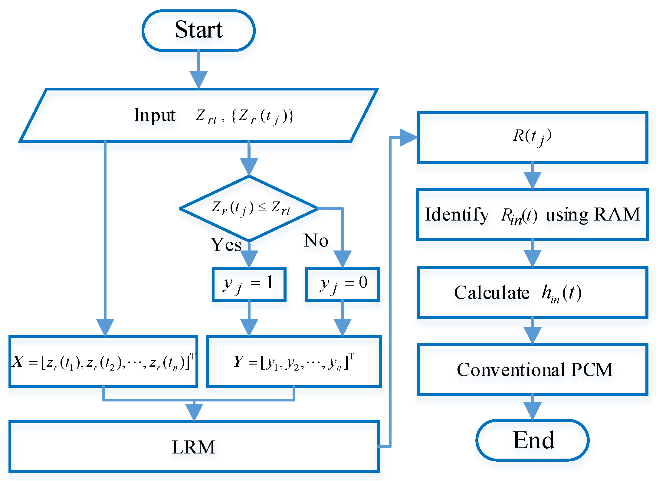
3.2. The IPCM Reliability Estimation Method

Under the circumstances of sparse or zero failure data, the key point of PCM is to determine the proportional factor r between the covariate and hazard rate for getting $C(t)$. From the point of the study, the reliability estimation method of PCM is theoretically feasible. However, being devoid of experiments and abundant experience of the experts, it is very hard to determine the proportional factor accurately. Through the introduction in Section 2.2, LRM may be a good choice to solve the problem.

The block diagram of the IPCM reliability assessment method is listed in Figure 2. Firstly, the salient feature indexes extracted from existing monitoring data are taken as input vectors of LRM to reflect the equipment operation performance. The equipment state variables determined by the failure threshold specified by the relevant standard or actual operation conditions are taken as the output of LRM. Then the initial reliability $R_{in}(t)$ can be estimated by LRM and incorporated into PCM to complete the process of reliability estimation. In the IPCM method, the initial hazard function $h_{i\mathrm{n}}(t)$ is evaluated only by using the existing condition information and asset state, which passes the decision process of the linear proportional factor r. The IPCM is independent of historical failure data and greatly expands using the scope of the PCM model for sparse or zero failure data.

The reliability estimation method based on IPCM is described as follows:

(1)

Input $Z_{rt}$ and $\{Z_r(t_j)\}\hspace{1em}(j=1,2,\cdots ,n)$, $Z_{rt}$ is the failure threshold of the response covariate and $\{Z_r(t_j)\}\hspace{1em}(j=1,2,\cdots ,n)$ is the response covariate dataset extracted from the monitoring data;

(2)

Identify the input vector $X$ and the output vector $Y$ of LRM, $X={[z_r(t_1),z_r(t_2),\cdots ,z_r(t_n)]}^{\mathrm{T}}$ and $Y={[y_1,y_2,\cdots ,y_n]}^{\mathrm{T}}$, if $Z_r(t_j)<Z_{rt}$, $y_j=1$ (under the normal state), otherwise $y_j=0$;

(3)

Estimate the parameters of LRM and calculate the concrete reliability $R(t_j)$ corresponding to $Z_r(t_j)$ by using Equation (10);

(4)

Identify the expression of $R_{in}(t)$ by using the regression analysis method (RAM).

(5)

Calculate the hazard function by equation $h_{in}(t)=f(t)/R_{in}(t)=-\mathrm{d}(\ln R_{in}(t))/\mathrm{d}t$ and implement the remaining reliability assessment procedures (4)~(6) of conventional PCM mentioned in Section 3.1, where $f(t)$ is the failure probability density function(PDF).

The algorithm of $h_{in}(t)$ shown in Figure 2 is illustrated in sole-response covariate form. For multi-dimension response covariates, the input $X={[Z_r(t_j)]}^{\mathrm{T}}\hspace{1em}(j=1,2,\cdots ,n)$ can be changed as $X={[Z_{ri}(t_j)]}^{\mathrm{T}}\hspace{1em}(i=1,2,\cdots ,K, j=1,2,\cdots ,n)$, K is the dimension of $X$. If the multivariate LRM is adopted, the proposed algorithm is still effective.

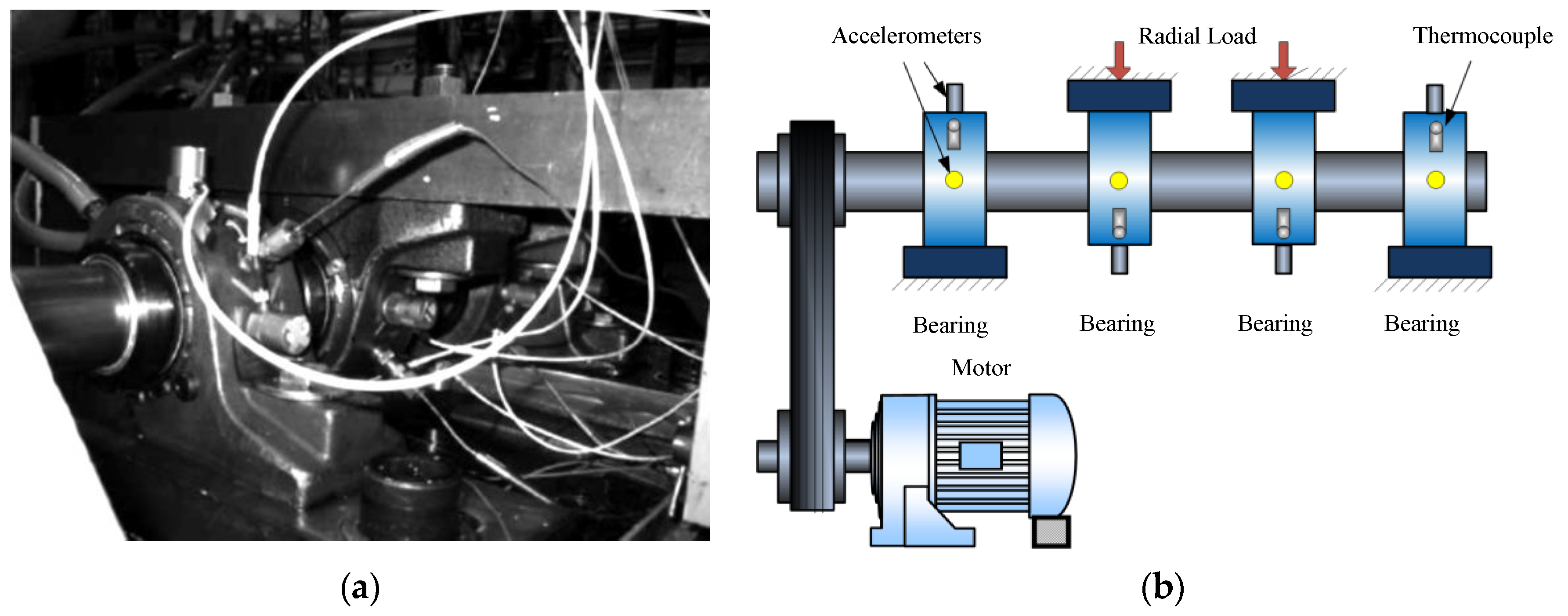
4. Case Study of Aero Engine Rolling Bearing

To verify the efficiency of the proposed improved PCM reliability assessment method under sparse or zero failure data condition, a case study is conducted on aero engine rolling bearing. The currently used maintenance strategy for aero engine rolling bearing is focused on controlling the flight hours or total cumulative cycle strictly to keep its stable performance due to the harsh working conditions. It is a highly conserved regular maintenance method [24]. Compared with failure life data, the operational condition data are easily obtained and can be used to characterize the performance degradation process of the individual bearing. If the salient features reflecting the degradation can be extracted by signal processing technology and taken as the input of the IPCM method, the mapping relationship between condition information and the system reliability will be built. It will be more suitable for industrial application in a single piece or small quantity equipment health assessment.

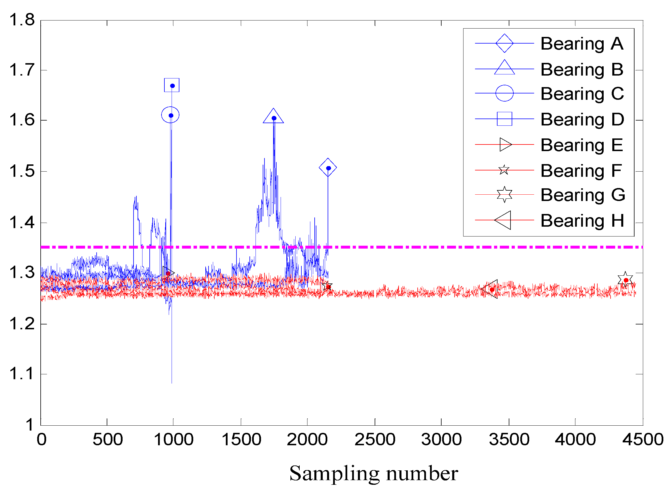
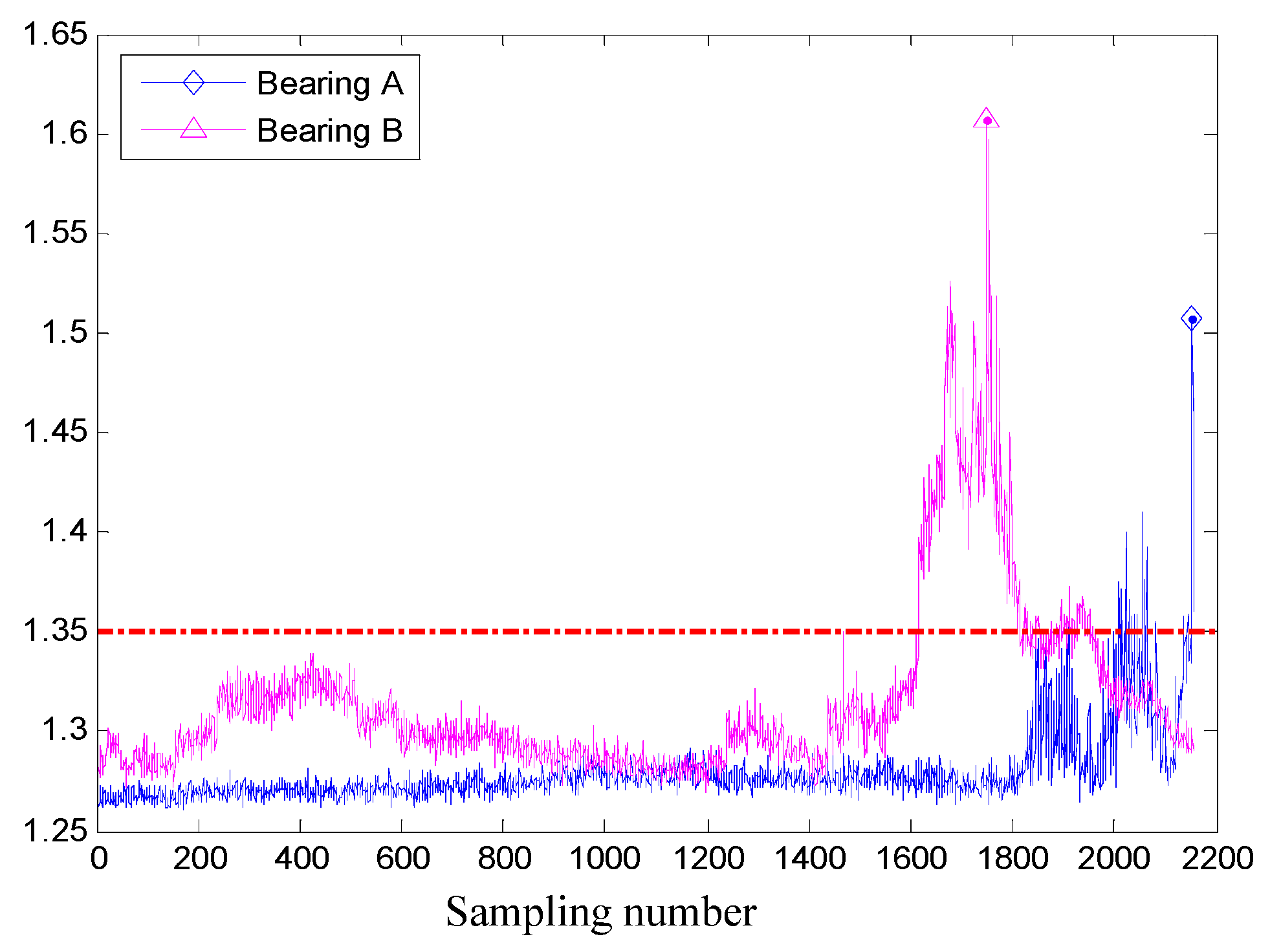
4.1. Data Description

The data come from UCR Center for Intelligent Maintenance Systems (IMS) [25]. The bearing test bench and sensor placement installations are shown in Figure 3. There are four ZA-2115 double row bearings were tested in the experiment. The structure parameters of the bearing are shown in

Table 1. The structure parameters of the rolling bearing.

Bearing Model	Pitch Diameter	Roller Diameter	Number of Rolling Element	Tapered Contact Angle
ZA-2115	2.815 in	0.331 in	16	15.17°

. The rotational speed was 2000 RPM and 6000 lb radial load was placed on the shaft by a spring mechanism. Eight PCB 353B33 ICP accelerometers were installed to collect the vibration signal. The data sampling frequency is 20 kHz, and the sampling points are 20,408. A magnetic plug was installed in the oil feedback pipe to collect debris from the oil as an indicator of bearing degradation. The test will stop when the accumulated debris adhered to the magnetic plug exceeds a certain level.

In the experiment, altogether, eight bearing’s vibration signals were acquired. Among them, only three bearings ran to failure and their lifetime varied quite a lot. It is a typical small sample failure data problem, and it is hard to estimate their reliability by using the conventional PCM model. In data set No. 1, an inner race defect was found in bearing 3 (labeled as bearing A), and a mixed roller element and outer race defect were observed in bearing 4 (labeled as bearing B). The remaining bearings are labeled as C~H.

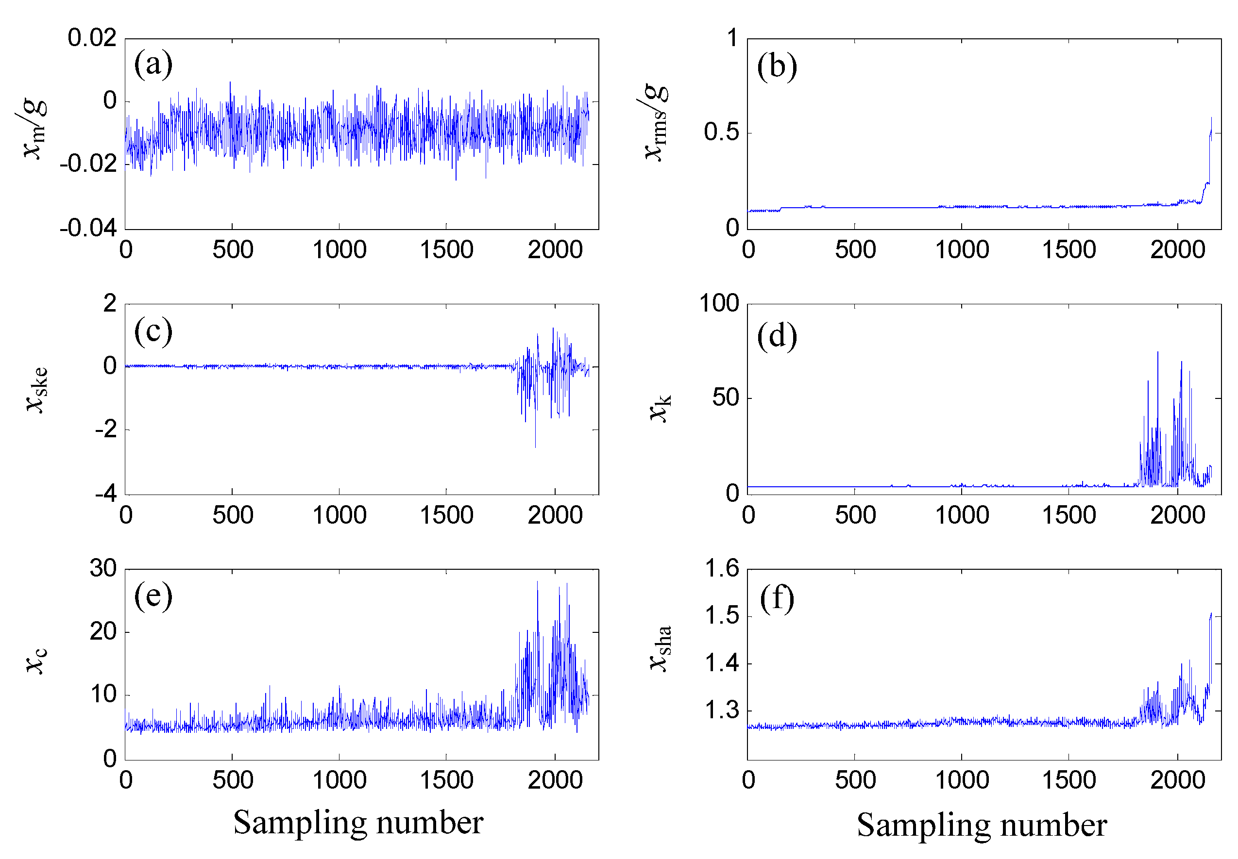
4.2. Data Analysis and Covariate Selection

Time-domain feature parameters are easy to calculate and commonly used in online conditional monitoring, which can reflect the working state of the rolling bearings [27]. Under normal circumstances, the amplitudes of the bearing vibration signals approximately obey a normal distribution with zero mean. If the bearing defect occurs, the amplitude of the time-domain signals will get larger [28]. The time domain features characterized by statistical analysis can be divided into dimensionless indicators and dimensional indicators [29]. The frequently used dimensional indicators include the mean, root mean square (rms) value, variance, etc. These values show a monotonically increasing trend with the increasing bearing failure. However, the dimensional indicators are sensitive and susceptible to the changes in load and rotational speed. Dimensionless indicators are substantially independent of rotational speed and load. The frequently used dimensionless time domain features include kurtosis indicator, peak indicator, and margin indicator, etc. [30]. In this section, there are 11 time-domain features are studied: Mean (x_m), peak (x_p), root amplitude (x_ra), root mean square (x_rms), standard deviation (x_std), skewness (x_ske), kurtosis (x_k), crest (x_c) margin (x_ma), shape (x_sha), and impulse factor (x_i). The mathematical descriptions of these features are shown in

Table 2. The time domain features.

$x_{\mathrm{m}}=\frac{{\displaystyle \sum _{n=1}^{N}x(n)}}{N}$	$x_{\mathrm{p}}=\max \left|x(n)\right|$	$x_{\mathrm{ra}}={(\frac{{\displaystyle \sum _{n=1}^N\sqrt{\left|x(n)\right|}}}{N})}^2$	$x_{\mathrm{xms}}=\sqrt{\frac{{\displaystyle \sum _{n=1}^N{(x(n))}^2}}{N}}$
$x_{\mathrm{std}}=\sqrt{\frac{{\displaystyle \sum _{n=1}^N{(x(n)-x_{\mathrm{m}})}^2}}{N-1}}$	$x_{\mathrm{ske}}=\frac{{\displaystyle \sum _{n=1}^N{(x(n)-x_{\mathrm{m}})}^3}}{(N-1)x_{\mathrm{std}}^3}$	$x_{\mathrm{k}}=\frac{{\displaystyle \sum _{n=1}^N{(x(n)-x_{\mathrm{m}})}^4}}{(N-1)x_{\mathrm{std}}^4}$	$x_{\mathrm{c}}=\frac{x_{\mathrm{p}}}{x_{\mathrm{rms}}}$
$x_{\mathrm{ma}}=\frac{x_{\mathrm{p}}}{x_{\mathrm{ra}}}$	$x_{\mathrm{sha}}=\frac{x_{\mathrm{rms}}}{x_{\mathrm{m}}}$	$x_{\mathrm{i}}=\frac{x_{\mathrm{p}}}{x_{\mathrm{m}}}$

where $x(n)$ is a time series $n=1,2,\dots ,N$, N is the number of data points.

.

The time domain feature extraction is applied to the vibration signals of bearing A. The above mentioned 11 time domain features have been calculated and only six representative feature figures are shown in Figure 4 because the other five features have similar changing trends to these six features. The similar relationships among them are listed in

Table 3. The similar relationships between different time domain features.

No.	1	2	3	4	5	6
similar relationships	xm	xrms,xra,xstd,xp	xske	xk	xc,xi,xmar	xsha

.

Since the sampling frequency is not uniformly spaced, the horizontal ordinate is expressed as the sampling number but not as real time. As is depicted in Figure 4, with the increase of operation time, different time domain features have apparently different changing trends. During the whole running process, x_m fluctuates extremely but has no obvious trend. The other five features are shown in Figure 4b–f. Their changing trends can be divided into two stages from the 1800th sampling number. x_rms nearly has no fluctuation but an apparently changing trend. Especially at the end of running, the values of x_rms increased monotonously from 0.15 to 0.6. On the contrary, x_ske fluctuates extremely but has no apparent changing trend. The amplitudes of x_k, x_c, and x_sha have some similar changing trends. In the first stage, their values are comparatively smaller. It means that the bearing operates healthily and normally. In the second stage, the amplitudes get larger, and the changing rate increases significantly. Two apparent crests can be clearly observed in Figure 4d–f. It means that the defects start emerging, propagating, and failing.

Generally speaking, the tendency of x_rms is the most obvious, while its susceptibility to incipient failure is the poorest. x_k is the most sensitive to incipient defect, but its tendency is not obvious. The tendency and susceptibility of x_c are comparatively good. However, it fluctuates extremely. Compared with the several above indicators, the sensitivity and the tendency of x_sha are relatively better, and the fluctuation is not very strong. Thus, it is selected as the response covariate.

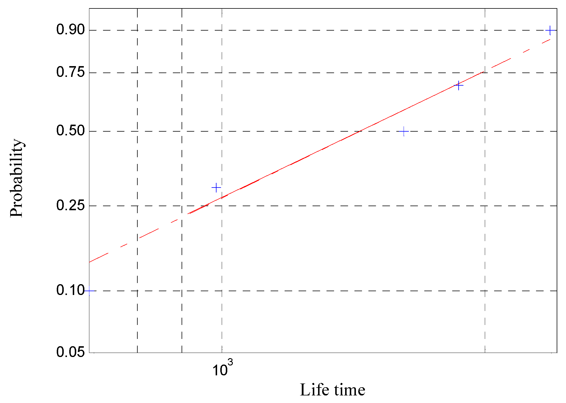
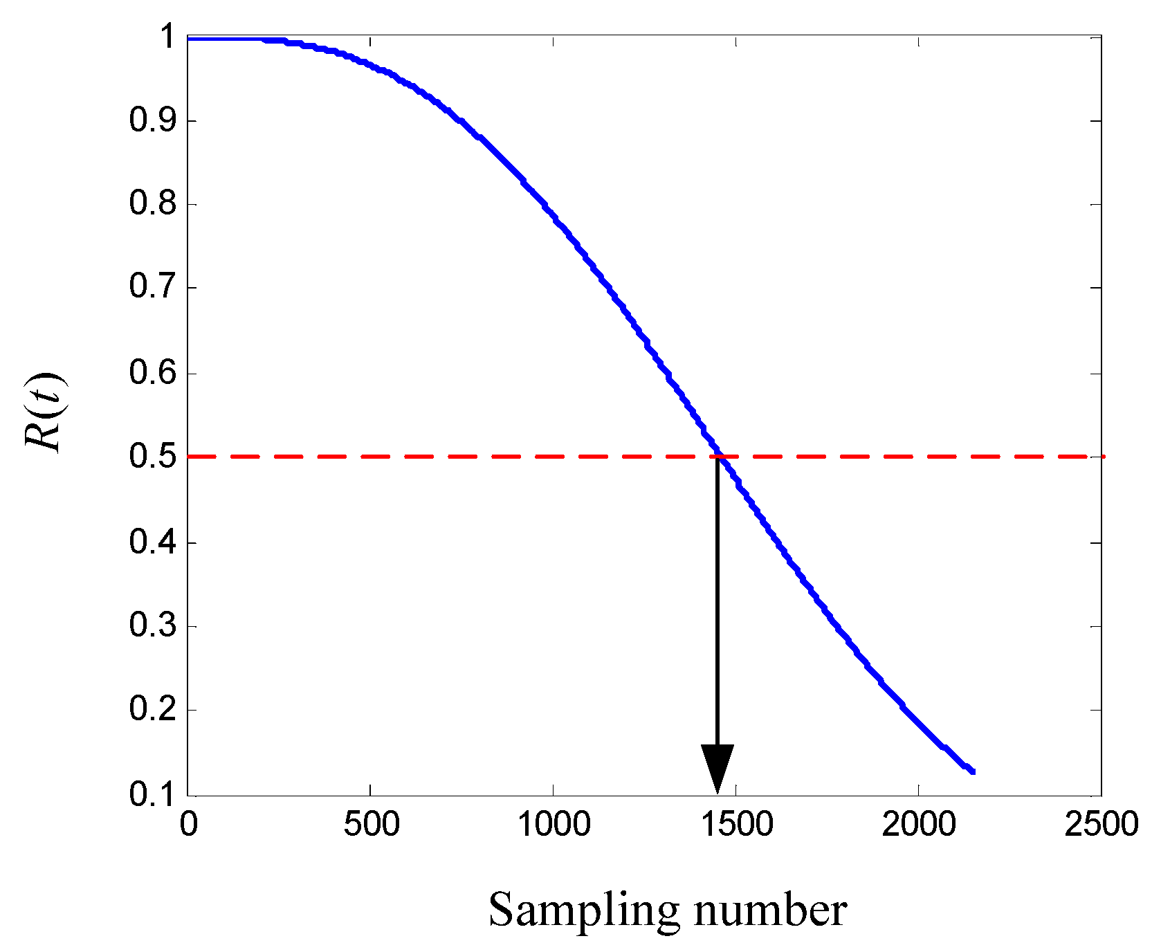
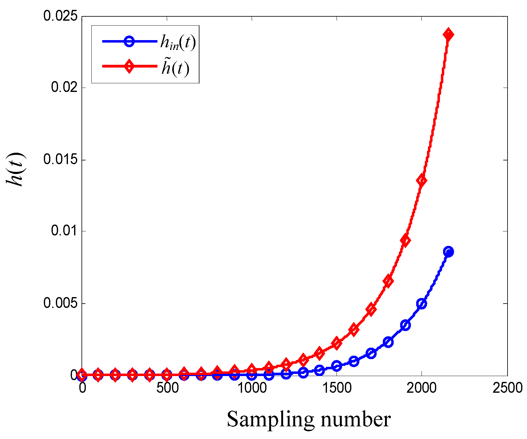
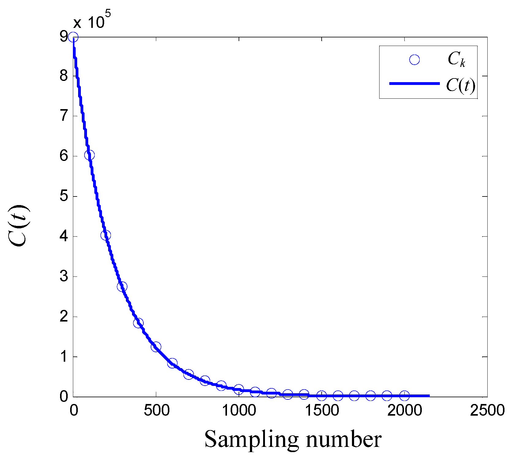
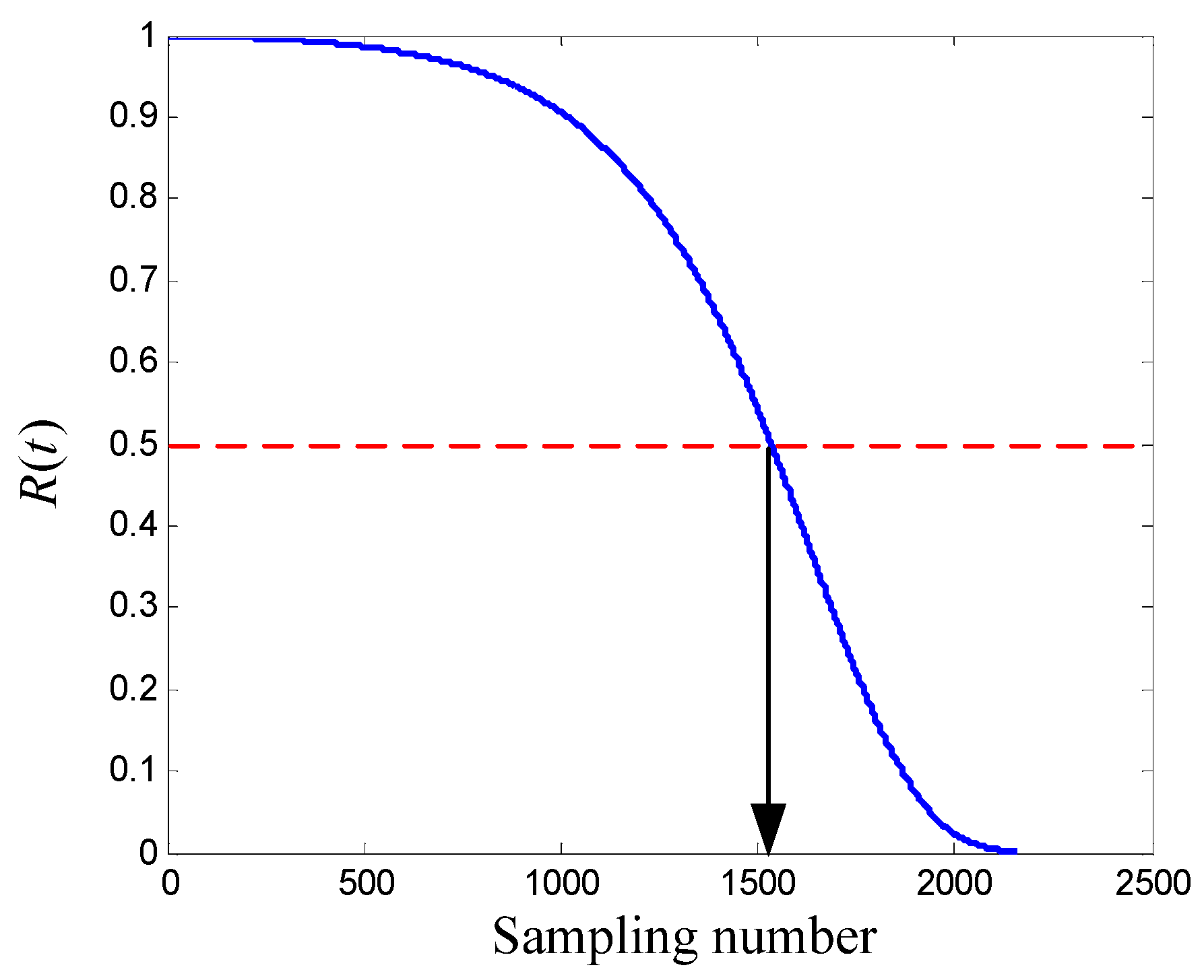
4.3. Reliability Estimation Based on Conventional PCM

According to Section 3.1, the failure life data should be acquired and used to evaluate the system initial hazard function $h_{in}(t)$. The degradation path model method [31] is considered to estimate the failure life for all the eight bearings labeled A~H. If the degradation of the equipment can be indicated by a condition feature, the equipment fails when the condition feature reaches a pre-set value, which is defined as the failure threshold [32]. The failure threshold has different identification criteria for different working situations. In [9], the flank wear value 0.6 mm is set as the failure threshold to identify the tool state with reference to ISO3685. In [33], the bearing running state can be classified into three different types, based on the maximum normalized shock value: Healthy (0 ≤ dB < 20), weak fault (20 ≤ dB < 35), and heavy fault (35 ≤ dB < 60). In [34], according to the industrial standard ISO 2372, an overall root mean square (rms) vibration acceleration level ranging between 2.0 and 2.2 Gs is considered a “danger level”. The vibration signals of the eight bearings have also been analyzed and their time domain features x_sha have been extracted and plotted together in Figure 5. In this study, we want to give an alarm threshold to trigger a preventive maintenance (PM) action (e.g., see [35]). As we can observe in Figure 5, the value 1.35 is suitable to select as the incipient failure threshold and is denoted as $x_{\mathrm{t}}$ in Figure 5 with a horizontal dot dash line. If $x_{s\mathrm{ha}}\le x_{\mathrm{t}}$, the bearing is considered normal. If $x_{s\mathrm{ha}}>x_{\mathrm{t}}$, the bearing is considered to have an incipient failure. Only the first four bearings A~D have reached the early failure criteria according to the incipient failure threshold. The failure lives of A~D determined by x_t are the 1864th, 1615th, 703th, and 983th sampling numbers, respectively. For the remaining bearings, the exponential function is employed to model the degradation process of the bearings. During the whole experimental period, the changing trends of x_sha of bearings F~H are not obvious. Thus, the degeneration path model fitting method is not available to obtain the incipient failure life. Only the degradation process of bearing E has been modeled as a biexponential function form.

$$x_{\mathrm{sha}}(t)=1.255\times e^{2.489\times {10}^{-6}t}+3.645\times {10}^{-18}\times e^{0.0159t}$$

(16)

The pseudo failure life of bearing E is the 2374 sampling number identified by x_t. Together with the previously mentioned four failure samples, there are five pieces of failure life data. The hypothesis test is implemented to analyze the failure distribution and the result is presented in Figure 6. It is rational to assume that the failure distribution of the bearings obeys a Weibull distribution, and the expression is shown as

$$F\left(t\right)=1-\exp \left[-{\left(\frac{t}{\eta }\right)}^{\beta }\right]=1-\exp \left[-{\left(\frac{t}{17008}\right)}^{2.8}\right]$$

(17)

Thus, the initial failure rate function of the bearings is

$$h_{in1}\left(t\right)=\frac{\beta }{\eta }{\left(\frac{t}{\eta }\right)}^{\beta -1}=\frac{2.8}{17008}{\left(\frac{t}{17008}\right)}^{1.8}$$

(18)

As described in Section 3.1, the discrete form of the baseline covariate function can be estimated based on $h_{in1}\left(t\right)$ and x_sha of the bearing A. The expression of the baseline covariate function by RAM for the bearing is listed as.

$$C_1(t)=4.962\times {10}^8{t}^{-1.8}$$

(19)

The response covariates $x_{\mathrm{sha}}$ of bearing B and $C_1(t)$ are introduced into Equation (13) to update $h_{in1}(t)$. Its continuous expression fitted by a power function curve is represented as

$${\tilde{h}}_1(t)=2.215\times {10}^{-9}{t}^{1.826}$$

(20)

The updated ${\tilde{h}}_1(t)$ is input into Equation (14) and the estimated reliability curve of bearing B is shown in Figure 7. If the threshold of reliability is selected as $R_{\mathrm{t}}=0.5$ [9], the estimated incipient failure time of bearing B is the 1465th sampling number. On the basis of the amount of the time accumulated debris, the actual incipient failure of bearings B is the 1615th sampling number. Supposing the sampling frequency is uniformly spaced. The estimation error is 9.29%.

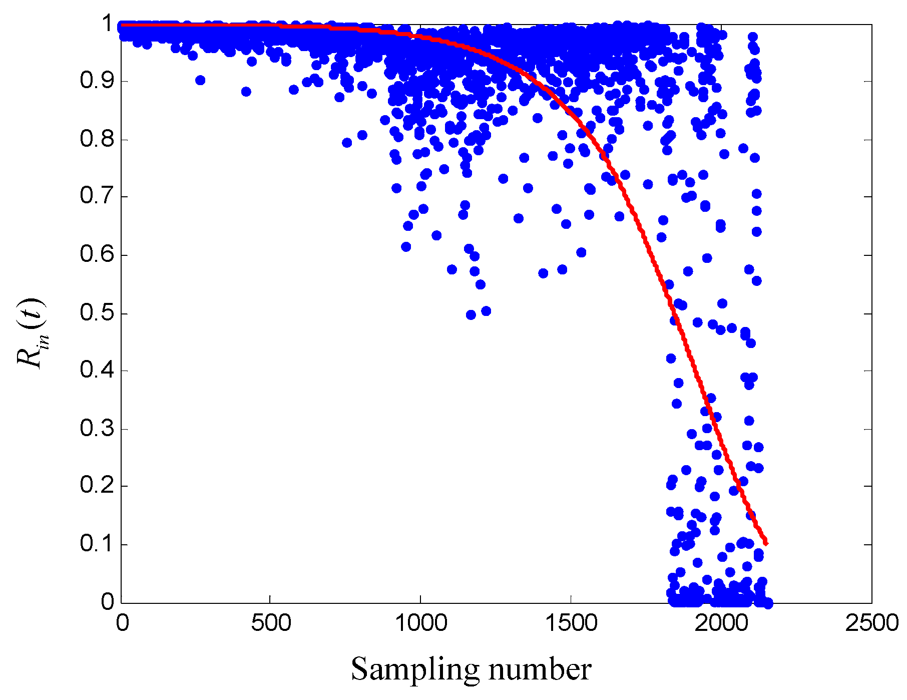
4.4. Reliability Estimation Based on IPCM

In order to compare with the results of the conventional PCM method, the IPCM reliability analysis method is also applied to bearing B. Similar to Section 4.2, the changing trends of x_sha of the first two failure bearings A and B are shown altogether in Figure 8. The failure starting points of bearings A and B determined by $x_{\mathrm{t}}$ are the 1864th and 1615th sampling numbers.

As the estimated procedure of IPCM described in Section 3.2, the vibration signals of the bearing A are taken as the existing information to calculate the initial hazard rate function $h_{in}(t)$. The vector X composed of shape factor $x_{\mathrm{sha}}^i$ at different sampling time t_i is taken as the input of the LRM. The vector Y composed of the bearing state variable y_i is taken as the output of the LRM (y_i is determined by the values of $x_{\mathrm{sha}}^i$ and $x_{\mathrm{t}}$. If $x_{s\mathrm{ha}i}<x_{\mathrm{t}}$, $y_i=1$, i.e., the bearing is normal, otherwise $y_i=0$). The model parameters are estimated by MLE and the obtained LRM is as follows.

$$\mathrm{Logit}(y_i)=\ln \frac{R(t_i|X_i)}{1-R(t_i|X_i)}=B{X}_i=271.4-210.2x_{\mathrm{sha}}^i$$

(21)

The reliability $R_{in2}(t_i)$ of the bearing A corresponding to different values of $x_{\mathrm{sha}}^i$ can be acquired based on Equation (10) and shown as the scatter diagram in Figure 9. Considering the descending trend of system reliability, one monotonous smooth curve can be used to fit the scatter diagram, shown as the solid lines in Figure 9. Then the discrete form of the initial hazard function $h_{in2}(t)$ can be calculated by equation $h_{in2}(t)=f(t)/R_{in2}(t)=-\mathrm{d}(\ln R_{in2}(t))/\mathrm{d}t$. Its continuous curve expression can be fitted by power function and exponential function and is described in

Table 4. The fitted model and parameters of $h_{in2}(t)$.

Model	$h_{in2}(t)=a{t}^b$	$h_{in2}(t)=a{e}^{bt}$
Parameters	a = 7.809 × 10−27  b = 7.212	a = 2.354 × 10−6 b = 0.003822
Goodness of fit:
SSE:	7.989 × 10−6	2.922 × 10−6
R-square:	0.999	0.9996
RMSE:	0.999	0.9996
Adjusted R-square:	6.091 × 10−5	3.684 × 10−5

. It can be found that the fitting goodness of the exponential function is superior to the power function. Therefore, it is selected as the function expression of $h_{in2}(t)$ and shown in Figure 10.

Just as the description in Section 3.2, once $h_{in2}(t)$ is obtained, the remaining reliability assessment procedures can be implemented by using the PCM method. The values of $x_{\mathrm{sha}}^i$ sever as the basic covariate and can be introduced into Equation (12) to calculate the discrete form $C_{k2}$ of the baseline covariate function. Its continuous function form $C_2(t)$ is fitted by an exponential model, whose advantages are more obvious than other models, as shown in Figure 11. The expression of $C_2(t)$ is

$$C_2(t)=8.994\times {10}^5{e}^{-0.003964t}$$

(22)

The response covariates $x_{\mathrm{sha}}$ of bearing B and $C(t)$ are simultaneously introduced into Equation (13) to update $h_{in2}(t)$. Considering the assumption that the covariates are proportional to the hazard of the system, the product factor expressed as $\exp (x_{\mathrm{sha}-\mathrm{B}}^i/x_{\mathrm{sha}-\mathrm{A}}^i)$ is introduced into the process of the hazard ratio function updating, where $x_{\mathrm{sha}-\mathrm{A}}^i$ and $x_{\mathrm{sha}-\mathrm{B}}^i$ are the shape values sampling time t_i of bearings A and B, respectively. Equation (13) has been changed as

$$\tilde{h}(t_i)=\frac{Z_r(t_i)}{C(t_i)}\exp (x_{\mathrm{sha}-\mathrm{B}}^i/x_{\mathrm{sha}-\mathrm{A}}^i)$$

(23)

Its continuous function fitted by the exponential curve is expressed as Equation (24) and shown in Figure 10.

$${\tilde{h}}_2(t)=9.811\times {10}^{-6}{e}^{3.613\times {10}^{-3}t}$$

(24)

The updated ${\tilde{h}}_2(t)$ is input into Equation (14) and the reliability of bearing B can be obtained. The estimated reliability curve is shown in Figure 12. Similar to Section 4.3, if the threshold of reliability is identified as $R_{\mathrm{t}}=0.5$, the estimated incipient failure time of bearing B is at the 1535th sampling number and the estimation error is 4.95%. Indeed, the assessment result of IPCM reliability is superior to the conventional PCM method.

The above reliability estimation process only involves the univariate condition. In Section 4.2, there are other 10 time domain features that have been analyzed. Through the signal processing method, we can also obtain more state characteristic indexes. The sensitivity, trends, and stability of the features are different. If some of them can be fused together to combine one or two new health indicator(s) (HI) with excellent properties, such as the MQE indicator used by Qiu and Lee [26] and the new HI obtained from the 6 AE features by Liu [36], the evaluative accuracy of the IPCM method will be increased. The fused methods, such as principal component analysis (PCA), factor analysis, distance analysis, and rough set, etc. [37,38], can be used for feature dimensionality reduction and extraction. In addition, because LMR is a multivariable model, this method is also feasible for multiple covariates.

It can be seen from the above comparative analysis that the conventional PCM analysis method relies on the failure life data excessively. Fewer failure samples will lead to a large deviation between the PDF of the failure life date estimated by the hypothesis and the actual PDF of the failure life. In the subsequent reliability assessment process, this deviation will be gradually transferred to the calculation of $h_{in}\left(t\right)$, $c\left(t\right)$, and ${\tilde{h}}_0\left(t\right)$, resulting in a large deviation between the actual evaluation reliability and the actual value.

5. Conclusions

The present study proposes a new kind of reliability assessment method named as IPCM under the condition of sparse or zero failure data. LRM is employed to calculate the initial hazard function and PCM is then employed to estimate the equipment’s operational reliability. Through the case studies of conventional PCM and IPCM to the aero engine rolling bearings, we can draw some conclusions as follows:

(1)

The LRM-based estimation method only needs acquiring the equipment’s response covariate vectors and their corresponding states without requiring specific mechanical knowledge or making many assumptions about the PDFs of variables. It passes the process of the proportional factor identification between covariate and hazard rate so that it can avoid the influence of the subjective deviation.

(2)

The salient features extracted and selected from conditional monitoring data during the equipment operation process are more suitable for the equipment degradation evaluation. The assessing accuracy of IPCM is superior to conventional PCM for a small failure sample, which verifies the plausibility and effectiveness of the proposed method. The method reveals the equipment performance from the conditional monitoring data and provides a new method for reliability assessment under sparse or zero failure data conditions.

(3)

This paper only studies the evaluation method and results of IPCM in the case of univariate. Some suggestions are given for the multivariable. The specific operation process and effectiveness need to be tested in future work.

References

1. Cerrada, M.; Sánchez, R.; Li, C.; Pacheco, F.; Cabrera, D.; de Oliveira, J.V.; Vásquez, R.E. A review on data-driven fault severity assessment in rolling bearings. Mech. Syst. Signal Process. 2018, 99, 169–196. [Google Scholar] [CrossRef]
2. Li, H.; Zuo, H.; Su, Y.; Xu, J.; Yin, Y. Study on segmented distribution for reliability evaluation. Chin. J. Aeronaut. 2017, 30, 310–329. [Google Scholar] [CrossRef]
3. Baussaron, J.; Mihaela, B.; Léo, G.; Fabrice, G.; Paul, S. Reliability assessment based on degradation measurements: How to compare some models? Reliab. Eng. Syst. Saf. 2014, 131, 236–241. [Google Scholar] [CrossRef] [Green Version]
4. Bhuyan, P.; Sengupta, D. Estimation of reliability with semi-parametric modeling of degradation. Comput. Stat. Data Anal. 2017, 115, 172–185. [Google Scholar] [CrossRef]
5. O’Connor, P.D. Commentary: Reliability-past, present, and future. IEEE Trans. Reliab. 2000, 49, 335–341. [Google Scholar] [CrossRef]
6. Zio, E. Reliability engineering: Old problems and new challenges. Reliab. Eng. Syst. Saf. 2009, 94, 125–141. [Google Scholar] [CrossRef] [Green Version]
7. Li, N.; Xu, P.; Lei, Y.; Cai, X.; Kong, D. A self-data-driven method for remaining useful life prediction of wind turbines considering continuously varying speeds. Mech. Syst. Signal Process. 2022, 165, 108315. [Google Scholar] [CrossRef]
8. Yan, T.; Lei, Y.; Li, N.; Wang, B.; Wang, W. Degradation Modeling and Remaining Useful Life Prediction for Dependent Competing Failure Processes. Reliab. Eng. Syst. Saf. 2021, 212, 107638. [Google Scholar] [CrossRef]
9. Chen, B.; Chen, X.; Li, B.; He, Z.; Cao, H.; Cai, G. Reliability estimation for cutting tools based on logistic regression model using vibration signals. Mech. Syst. Signal Process. 2011, 25, 2526–2537. [Google Scholar] [CrossRef]
10. Sy, J.P.; Taylor, J.M. Estimation in a Cox proportional hazards cure model. Biometrics 2000, 56, 227–236. [Google Scholar] [CrossRef]
11. Kumar, D.; Klefsjö, B. Proportional hazards model: A review. Reliab. Eng. Syst. Saf. 1994, 44, 177–188. [Google Scholar] [CrossRef]
12. Lin, D.; Banjevic, D.; Jardine, A.K. Using principal components in a proportional hazards model with applications in condition-based maintenance. J. Oper. Res. Soc. 2006, 57, 910–919. [Google Scholar] [CrossRef]
13. Zhang, Q.; Hua, C.; Xu, G. A mixture Weibull proportional hazard model for mechanical system failure prediction utilising lifetime and monitoring data. Mech. Syst. Signal Process. 2014, 43, 103–112. [Google Scholar] [CrossRef]
14. Banjevic, D.; Jardine, A.; Makis, V.; Ennis, M. A control-limit policy and software for condition-based maintenance optimization. INFOR Inf. Syst. Oper. Res. 2001, 39, 32–50. [Google Scholar] [CrossRef]
15. Ding, F.; He, Z. Cutting tool wear monitoring for reliability analysis using proportional hazards model. Int. J. Adv. Manuf. Technol. 2011, 57, 565–574. [Google Scholar] [CrossRef]
16. Sun, Y.; Ma, L.; Mathew, J.; Wang, W.; Zhang, S. Mechanical systems hazard estimation using condition monitoring. Mech. Syst. Signal Process. 2006, 20, 1189–1201. [Google Scholar] [CrossRef]
17. Cai, G.; Chen, X.; Li, B.; Chen, B.; He, Z. Operation reliability assessment for cutting tools by applying a proportional covariate model to condition monitoring information. Sensors 2012, 12, 12964–12987. [Google Scholar] [CrossRef] [Green Version]
18. Rabbani, M.; Manavizadeh, N.; Balali, S. A stochastic model for indirect condition monitoring using Proportional Covariate model. IJE Trans. A Basics 2008, 21, 45–56. [Google Scholar]
19. Yan, J.; Lee, J. Degradation assessment and fault modes classification using logistic regression. J. Manuf. Sci. Eng. 2005, 127, 912–914. [Google Scholar] [CrossRef]
20. Liao, H.; Zhao, W.; Guo, H. Predicting remaining useful life of an individual unit using proportional hazards model and logistic regression model. In Proceedings of the RAMS’06 Annual Reliability and Maintainability Symposium, Newport Beach, CA, USA, 23–26 January 2006; pp. 127–132. [Google Scholar]
21. Wang, F.; Wang, B.; Dun, B.; Chen, X.; Yan, D.; Zhu, H. Remaining life prediction of rolling bearing based on PCA and improved logistic regression model. J. Vibroeng. 2016, 18, 5192–5203. [Google Scholar] [CrossRef]
22. Myers, R.H.; Montgomery, D.C.; Vining, G.G.; Robinson, T.J. Generalized Linear Models: With Applications in Engineering and the Sciences; John Wiley & Sons: Hoboken, NJ, USA, 2012; ISBN 0470556978. [Google Scholar]
23. Menard, S. Applied Logistic Regression Analysis; Sage: Thousand Oaks, CA, USA, 2002; ISBN 0761922083. [Google Scholar]
24. Xuewen, M.; Cong, N.; Yun, Y.; Lei, H.; Jie, H. Grade-lfe prognostic model of aircraft engine bearing. Trans. Nanjing Univ. Aeronaut. Astronaut. 2012, 29, 171–178. [Google Scholar]
25. Lee, J.; Qiu, H.; Yu, G.; Lin, J. Bearing Data Set’, IMS; University of Cincinnati: Cincinnati, OH, USA, 2007. [Google Scholar]
26. Qiu, H.; Lee, J.; Lin, J.; Yu, G. Robust performance degradation assessment methods for enhanced rolling element bearing prognostics. Adv. Eng. Inform. 2003, 17, 127–140. [Google Scholar] [CrossRef]
27. Lei, Y.; Lin, J.; Zuo, M.J.; He, Z. Condition monitoring and fault diagnosis of planetary gearboxes: A review. Measurement 2014, 48, 292–305. [Google Scholar] [CrossRef]
28. He, Q.; Ding, X. Sparse representation based on local time–frequency template matching for bearing transient fault feature extraction. J. Sound Vib. 2016, 370, 424–443. [Google Scholar] [CrossRef]
29. Xue, X.; Zhou, J. A hybrid fault diagnosis approach based on mixed-domain state features for rotating machinery. ISA Trans. 2017, 66, 284–295. [Google Scholar] [CrossRef]
30. Lei, Y.; He, Z.; Zi, Y.; Hu, Q. Fault diagnosis of rotating machinery based on multiple ANFIS combination with GAs. Mech. Syst. Signal Process. 2007, 21, 2280–2294. [Google Scholar] [CrossRef]
31. Gorjian, N.; Ma, L.; Mittinty, M.; Yarlagadda, P.; Sun, Y. A review on degradation models in reliability analysis. In Engineering asset Lifecycle Management; Springer: Berlin/Heidelberg, Germany, 2010; pp. 369–384. [Google Scholar]
32. Jiang, R.; Jardine, A.K. Health state evaluation of an item: A general framework and graphical representation. Reliab. Eng. Syst. Saf. 2008, 93, 89–99. [Google Scholar] [CrossRef]
33. Li, Z.; He, Z.; Zi, Y.; Chen, X. Bearing condition monitoring based on shock pulse method and improved redundant lifting scheme. Math. Comput. Simul. 2008, 79, 318–338. [Google Scholar]
34. Gebraeel, N.Z.; Lawley, M.A. A neural network degradation model for computing and updating residual life distributions. IEEE Trans. Autom. Sci. Eng. 2008, 5, 154–163. [Google Scholar] [CrossRef]
35. Jiang, R. Optimization of alarm threshold and sequential inspection scheme. Reliab. Eng. Syst. Saf. 2010, 95, 208–215. [Google Scholar] [CrossRef]
36. Liu, Y.; Hu, X.; Zhang, W. Remaining useful life prediction based on health index similarity. Reliab. Eng. Syst. Saf. 2019, 185, 502–510. [Google Scholar] [CrossRef]
37. Chen, B.; Shen, B.; Zhang, F.; Xiao, W.; Chen, F.; Tian, H.; Chen, S. Operation reliability evaluation of cutting tools based on singular value decomposition transform and support vector space. Proc. Inst. Mech. Eng. Part O J. Risk Reliab. 2019, 233, 175–185. [Google Scholar] [CrossRef]
38. Thangavel, K.; Pethalakshmi, A. Dimensionality reduction based on rough set theory: A review. Appl. Soft Comput. 2009, 9, 1–12. [Google Scholar] [CrossRef]
Figure 1. The flow diagram of PCM reliability estimation.
Machines 10 00337 g001
Figure 2. The flowchart of the reliability estimation method based on IPCM.
Machines 10 00337 g002
Figure 3. Bearing test bench and sensor installation (a) the picture of test bench (b) the structure chart of test bench and sensor installation. Reprinted from Qiu, H.; Lee, J.; Lin, J.; Yu, G. (2003) [26].
Machines 10 00337 g003
Figure 4. The time domain features extracted from the vibration signals of bearing A (a) xm, (b) xrms, (c) xske, (d) xk, (e) xc, (f) xsha.
Machines 10 00337 g004
Figure 5. The time domain features xsha of the eight bearings.
Machines 10 00337 g005
Figure 6. The fitted Weibull distribution of the failure life data.
Machines 10 00337 g006
Figure 7. The estimated reliability of bearing B based on PCM.
Machines 10 00337 g007
Figure 8. The time domain features xsha of the two failure bearings.
Machines 10 00337 g008
Figure 9. The scatter diagram and the fitted function of initial reliability R i n 2 ( t ) .
Machines 10 00337 g009
Figure 10. The initial hazard function h i n 2 ( t ) and its updated form h ˜ 2 ( t ) .
Machines 10 00337 g010
Figure 11. The discrete form Ck2 and the continuous function form C2(t) of baseline covariate function.
Machines 10 00337 g011
Figure 12. The estimated reliability of bearing B based on improved PCM.
Machines 10 00337 g012