An Object Detection Model for Paint Surface Detection Based on Improved YOLOv3

Abstract

To solve the problem of poor performance of the target detection algorithm and false detection in the detection of paint surface defects of office chairs five-star feet, we propose a defect detection method based on the improved YOLOv3 algorithm. Firstly, a new feature fusion structure is designed to reduce the missed detection rate of small targets. Then we used the CIOU loss function to improve the positioning accuracy. At the same time, a parallel version of the k-means++ initialization algorithm (K-means||) is used to optimize and determine the parameters of the a priori anchor so as to improve the matching degree between the a priori anchor and the feature layer. We constructed a dataset of paint surface defects on the five-star feet of office chairs and performed optimization training, and used multiple algorithms and different datasets to conduct comparative experiments to validate the algorithm. The experimental results show that the improved YOLOv3 algorithm is effective in that the average precision on the self-made dataset reaches 88.3%, which is 5.8% higher than the original algorithm. At the same time, it has also been verified based on the Aliyun Tianchi competition aluminum dataset, and the average precision has reached 89.2%. This method realizes the real-time detection of the paint surface defects of the five-star feet of the office chair very well.

1. Introduction

In the field of industrial production, with the development of information technology, the application of big data in industrial manufacturing has gradually become an essential method of intelligent production. In the office chair manufacturing industry, the appearance quality of the office chair has a significant impact on the sales of its products. The paint defect detection of the five-star feet is an essential part of improving the overall appearance quality of the office chair, so the paint surface of the five-star feet needs to be inspected. In detecting paint surface defects of office chair five-star feet, the traditional detection method relies on artificial eyes to execute. It can only be judged by existing standards and common sense, which requires workers to have sufficient experience and common sense. It requires long-term concentration and is prone to fatigue, resulting in misjudgment. Therefore, the efficiency of manual detection is very low, and the cost will increase in the long run.

Traditional target detection methods mainly use manual extraction of signs and then detection by sliding window. It primarily consists of region selection, feature extraction, and classifier. However, it has apparent shortcomings: in natural scenes, it is often difficult to extract features due to factors such as occlusion and distance, the region selection strategy based on the sliding window is not targeted, the amount of calculation is large, the time complexity is high, the window is redundant, it does not have good robustness, and there are often missed detections and false detections during detection.

With the development of computer technology, deep learning, and the rapid improvement of GPU computing power, it is possible to apply deep learning-based defect detection methods in industrial manufacturing. The task of object detection is to find all objects of interest in an image and determine their location, size, and category information. With the rise of deep learning, the extracted deep features have more powerful representation capabilities than traditional handcrafted features. Target detection algorithms based on deep learning have gradually become the mainstream target detection algorithms. In addition, it can be divided into two categories, the first category is the two-stage target detection algorithm, and the representative algorithm is R-CNN (region-convolution neural network) [1,2], Fast R-CNN [3], Faster R-CNN [4,5], etc. These algorithms have low recognition error and miss recognition rates, but the detection speed is slow and cannot be performed in real-time detection. The second category is single-stage object detection algorithms [6], which can also be called end-to-end object detection algorithms. It does not require the stage of generating candidate regions. Still, it directly generates the object category’s probability and coordinate position values, and the final result can be obtained in a single detection. Therefore, the detection speed of this type of algorithm is faster, and the representative algorithms are SSD (Single Shot MultiBox Detector) [7,8], YOLO (You Only Look Once) [9,10], YOLOv2 [11], YOLOv3 [12,13,14,15,16,17], YOLOv4 [18], etc. Due to the structure of the YOLOv3 algorithms being more concise than the alternatives, it is more widely used in the industry. Although the detection performance of YOLOv3 is not as good as that of YOLOv4 [19,20,21], its transmission path is simple, and its versatility is strong. Therefore, the YOLOV3 algorithm is selected as the basis for the research method of the paint surface defect detection of the five-star feet of the office chair in this paper.

Although the target detection algorithm has developed a lot, there are still some problems to be solved, such as the research on small target detection not being mature, the resolution of small targets being low, and the proportion of pixels being small. The resolution of small targets is low, and the effective information that can be obtained during the target detection process is small. Due to the large deep receptive field in the convolutional neural network, it is difficult to extract the features of small targets after multiple down sampling. Therefore, the target detection algorithm is still poor for small-sized target recognition, and detection errors often occur [22,23].

In order to solve the problem of small target detection, Zhang Xu [24] and others proposed to add an anchor in each scale of YOLOv3 to improve the detection accuracy of small targets. Li Weigang [25] and others proposed to fuse shallow features and in-depth features to form a new large-scale detection layer, use a new clustering algorithm to optimize and determine a priori frame parameters, and finally achieve the purpose of improving detection accuracy. Xu Lifeng [26] and others proposed to build a feature pyramid structure in dense blocks of different levels of DenseNet, combining the high resolution of low-level features and the high semantics of high-level features and introducing soft threshold non-maximum suppression to improve the detection rate and accuracy. In the current research, it is usually considered an optimization and improvement to the YOLOv3 algorithm when combining new structures or functions.

On the basis of previous research, this paper uses the improved deep learning algorithm YOLOv3 to detect small objects. The improvement directions include network structure, clustering algorithm, and bounding box loss function. Firstly, the clustering algorithm is optimized to obtain better anchor boxes, improving average detection accuracy and speed. Secondly, the network structure is improved to enhance the small target detection performance. Finally, the bounding box loss function is improved to improve the positioning accuracy and the overall detection effect. In addition, we constructed a dataset of paint surface defects on the five-star feet of office chairs and performed optimization training and validation.

2. Principle of the YOLOv3 Algorithm

2.1. Detection Principle

YOLOv3 integrates the feature pyramid network (FPN), residual network (ResNet), and other methods, extracts multiple feature detection layers of different scales for detection, and improves the algorithm’s ability to detect targets of various sizes. The YOLOv3 algorithm can predict the category and location of objects while generating candidate regions. It does not need to be divided into two stages to complete the detection task and achieve end-to-end detection. YOLOv3 is mainly composed of a prediction network and darknet-53 feature extraction network. The network structure of YOLOv3 is shown in Figure 1.

Darknet-53 eliminates gradient dispersion with five residual blocks, and its network structure is shown in Figure 2 [14]. The Darknet-53 network is the core idea of the YOLOv3 algorithm. Its structure includes multiple convolutional layers, and the output YOLO layer image has three scales: small, medium, and large. Therefore, even if some of the detected feature information is lost or interfered with by external influences and other factors, the target can be detected.

2.2. Loss Function

The loss function is usually used to evaluate the model’s actual and predicted values. The loss function plays a vital role in the network learning speed and the final model prediction effect. The loss function of YOLOv3 is shown in Equation (1).

$$\begin{gathered} Loss={\lambda }_{coord}{{\displaystyle \sum }}_{i=0}^{S^2}{{\displaystyle \sum }}_{j=0}^B{I}_{ij}^{obj}[{(x_i^j-{\widehat{x}}_i^j)}^2+{\left(y_i^j-{\widehat{y}}_i^j\right)}^2] \\ +{\lambda }_{coord}{{\displaystyle \sum }}_{i=0}^{S^2}{{\displaystyle \sum }}_{j=0}^B{I}_{ij}^{obj}[{\left(\sqrt{w_i^j}-\sqrt{{\widehat{w}}_i^j}\right)}^2+{\left(\sqrt{h_i^j}-\sqrt{{\widehat{h}}_i^j}\right)}^2] \\ -{\displaystyle \sum }_{i=0}^{S^2}{\displaystyle \sum }_{j=0}^B{I}_{ij}^{obj}[{\widehat{C}}_i^{j}log\left(C_i^j\right)+\left(1-{\widehat{C}}_i^j\right)log\left(1-C_i^j\right)] \\ -{\lambda }_{noobj}{{\displaystyle \sum }}_{i=0}^{s^2}{{\displaystyle \sum }}_{j=0}^B{I}_{ij}^{noobj}[{\widehat{C}}_i^{j}log\left(C_i^j\right)+\left(1-{\widehat{C}}_i^j\right)log\left(1-C_i^j\right)] \\ -{\displaystyle \sum }_{i=0}^{S^2}{I}_{ij}^{obj}{\displaystyle \sum }_{C\in classes}\left(\left[{\widehat{P}}_i^{j}log\left(P_i^j\right)+\left(1-{\widehat{P}}_i^j\right)log\left(1-P_i^j\right)\right]\right) \end{gathered}$$

(1)

In Equation (1), S represents the grid size; that is, $S^2$ represents 13 × 13, 26 × 26, 52 × 52. B represents the number of prediction frames. $I_{i,j}^{obj}$ indicates the probability that the box appears at i, j, if it is not 0, it is 1, $I_{i,j}^{noobj}$ is the same as $I_{i,j}^{obj}$, on the contrary, it represents the probability that the box has no target at i, j, which is either 0 or 1. $w_i^j、h_i^j \mathrm{and} \widehat{w_i^j}、\widehat{h_i^j}$ represent the width and height of the prediction frame and the real frame, respectively. ${\widehat{C}}_i^j$ represents the real value, and the value of ${\widehat{C}}_i^j$ is determined by whether the Bounding Box in the grid is responsible for predicting an object. If it is responsible, it is ${\widehat{C}}_i^j$, otherwise, it is 0. $P_i^j$ and ${\widehat{P}}_i^j$ represent the predicted value and the actual value of the predicted target probability, respectively. 𝜆_{𝑐𝑜𝑜𝑟𝑑} and 𝜆_{𝑛𝑜𝑜𝑏𝑗} denote the weights of bounding box loss and confidence loss, respectively.

3. Improvement of YOLOv3 Algorithm

3.1. Improvement of Network Structure

Because the paint surface of the five-star feet of the office chair has small defect types, and because the down sampling multiple of the original YOLOv3 algorithm is too large, it creates a large receptive field of the feature map, resulting in a poor detection effect of small targets and missed detections. The YOLOv3 algorithm draws on the FPN method and uses multi-scale feature maps to detect objects of different sizes to improve the prediction ability of small objects. It obtains three feature maps of different scales by down sampling 32 times, 16 times, and 8 times, and the feature map of each scale will predict three priors’ anchor. This paper will improve the YOLOv3 algorithm by extending one scale to achieve small target detection.

On the basis of the 52 × 52 feature map obtained by eight times the down sampling, the 104 × 104 feature map is obtained by two times the up sampling. Then, it is stacked and fused with the 104 × 104 feature map obtained by down sampling the backbone network four times, and it is predicted from the feature map obtained this time. There are a total of 118 fully convolutional layers after the network improvement. Moreover, it has four different feature scales for independent prediction after improvement. It realizes the multiplexing of shallow information and can perform regression classification on the feature map after four times the down sampling, so as to achieve the purpose of enhancing the detection ability of small objects. The improved network structure is shown in Figure 3, and the part marked by the dotted box in the figure is the newly added feature scale.

3.2. Improvement of Bounding Box Loss Function

The IOU loss is an important indicator in object detection, which mainly describes the overlapping area of the predicted anchor and the ground-truth anchor. That is, the IOU is calculated by the ratio of the intersection and union between the predicted box and the ground-truth box and is often used to evaluate the pros and cons of the bounding box, as shown in Equation (2).

$$\mathrm{IOU}=\frac{\left|\mathrm{A}\cap \mathrm{B}\right|}{\left|\mathrm{A}\cup \mathrm{B}\right|}$$

(2)

In Equation (2), A and B represent the predicted anchor and the real anchor, respectively. The IOU is scale-invariant, but if the two boxes do not intersect, as shown in Figure 4, the values of IOU of the A box and the B box, and the A box and the C box are all 0. However, at this time, the distance between the B box and the C box is closer than the distance between the A box and the B box, and the IOU cannot calculate the distance between the two bounding boxes. In addition, the fine-tuning of the bounding box adopts the L2 norm. When there is no intersection of the real boxes, the IOU value is 0, and the gradient when optimizing the loss function is also 0, so learning and training cannot be performed.

GIOU [27] is optimized on the basis of IOU. Figure 5 shows the regression process of GIOU and CIOU, in which box a is the target box, box b is the anchor box, and box c is the offset result of the anchor box after different iterations. Moreover, both GIOU and CIOU can guide the detection anchor movement. GIOU adjusts the prediction anchor by position, aspect ratio, size, etc. As shown in Figure 5, during the regression process of GIOU, when the IOU is 0, GIOU first allows the anchor to overlap with the target anchor. Then GIOU will gradually degenerate into an IOU regression strategy, so the whole process will be slow, and there is a risk of divergence. Therefore, the idea of CIOU is introduced to solve the problem. CIOU is based on DIOU [28] and considers the width–length ratio in the three elements of bounding box regression, while DIOU considers the center distance information of the bounding box on the basis of IOU. CIOU quickly pulls back the position without changing the shape of the prediction frame, so CIOU pulls back the prediction frame faster than GIOU and makes its IOU greater than 0. When the IOU is greater than 0, CIOU will quickly adjust the size. When the IOU is more significant than 0.5, the aspect ratio part of the CIOU will start to be the main part of the gradient propagation so that the prediction box and the target box have the same aspect ratio. Moreover, CIOU is a better evaluation standard at present, so this paper will use CIOU to replace IOU in the original algorithm.

The CIOU loss function equation is shown in Equation (3).

$$L_{CIOU}=1-IOU+\frac{{\rho }^2\left(b,b^{gt}\right)}{c^2}+\alpha v$$

(3)

In Equation (3), ${\rho }^2\left(b,b^{gt}\right)$ represents the Euclidean distance between the center points of the prediction frame and the real frame, respectively, and C represents the diagonal distance of the minimum closure area that can contain the prediction frame and the real anchor at the same time. α is the weight function and v is the parameter to measure the consistency of the aspect ratio. α as shown in Equation (4), v as shown in Equation (5), and $\omega ,h and {\omega }^{gt},h^{gt}$ in Equation (5) represent the width and height of the prediction anchor and the real anchor, respectively. In Equation 5, $\omega and h$ represent the width and height of the predicted frame, and ${\omega }^{gt}and h^{gt}$ represent the width and height of the real frame.

$$\alpha =\frac{v}{\left(1-IOU\right)+v}$$

(4)

$$v=\frac{4}{{\pi }^2}{\left(arctan\frac{{\omega }^{gt}}{h^{gt}}-arctan\frac{\omega }{h}\right)}^2$$

(5)

The modified loss function is shown in Equation (6).

$$\begin{gathered} Loss={{\displaystyle \sum }}_{i=0}^{s^2}{{\displaystyle \sum }}_{j=0}^B{I}_{ij}^{obj}\left(1-IOU+\frac{{\rho }^2\left(b,b^{gt}\right)}{c^2}+\alpha v\right)*(2-{\widehat{w}}_i^j{\widehat{h}}_i^j) \\ -{\displaystyle \sum }_{i=0}^{S^2}{\displaystyle \sum }_{j=0}^B{I}_{ij}^{obj}[{\widehat{C}}_i^{j}log\left(C_i^j\right)+\left(1-{\widehat{C}}_i^j\right)log\left(1-C_i^j\right)] \\ -{\lambda }_{noobj}{{\displaystyle \sum }}_{i=0}^{s^2}{{\displaystyle \sum }}_{j=0}^B{I}_{ij}^{noobj}\left[{\widehat{C}}_i^{j}log\left(C_i^j\right)+\left(1-{\widehat{C}}_i^j\right)log\left(1-C_i^j\right)\right] \\ -{{\displaystyle \sum }}_{i=0}^{S^2}{I}_{ij}^{obj}{{\displaystyle \sum }}_{C\in classes}\left(\left[{\widehat{P}}_i^{j}log\left(P_i^j\right)+\left(1-{\widehat{P}}_i^j\right)log\left(1-P_i^j\right)\right]\right) \end{gathered}$$

(6)

3.3. Improvement of Clustering Algorithm

The YOLOv3 algorithm uses the K-means clustering algorithm to cluster and select anchor boxes. On the COCO dataset, nine kinds of priors’ anchors are obtained by clustering, and the allocation of priors’ anchors is shown in

Table 1. Priors anchor assignment.

Feature Map	Receptive Field	A Priori Box Size
13 × 13	Big	(116 × 90), (156 × 198), (373 × 326)
26 × 26	Middle	(30 × 61), (62 × 45), (59 × 119)
52 × 52	Small	(10 × 13), (16 × 30), (33 × 23)

.

The K-means algorithm randomly determines the initial clustering centers. Different clustering centers will lead to different clustering results, which may lead to slower convergence of the clustering algorithm and clustering errors. Therefore, the K-means++ [29,30] algorithm is proposed to solve the problem so that the distance between the cluster centers is far enough, and the distance is defined as follows.

$$d=1-GIOU\left(box,centroid\right)$$

(7)

However, since the selection of the next center point in the K-means++ algorithm depends on the center point that has been selected, in order to solve this defect, the K-means|| algorithm is used to solve it. The K-means|| algorithm is a variant of the K-means++ algorithm. The main idea of the algorithm is to change the sampling strategy for each traversal. Instead of taking out only one sample per traversal as in K-means++, each traversal takes O(k) samples. This paper will adopt the K-means|| algorithm, and its steps are shown in Algorithm 1.

Algorithm 1 K-means||

Input: DATA X; clusters K; oversampling l.

Output: set of prototypes C = {c1,c2,…,ck}.

1. Uniformly and randomly select a sample from X as a candidate cluster center C.

2.  $\psi \leftarrow$compute ${\varnothing }_X\left(C\right)$

3. for $O\left(log\left(\psi \right)\right)$ times do

4. $\mathrm{C}$sample each point $x\in X$ independently with probability $p_x=\frac{l·d^2\left(x,C\right)}{{\varphi }_X\left(C\right)}$

5. $\mathrm{C}\leftarrow$$\mathrm{C}’\cup$C

6. end for

7. Run the weighted K-means++ algorithm on the set of candidate centers to get the exact K cluster centers.

8. Run the standard K-means algorithm with the resulting K cluster centers.

Calculate $\psi$ in step 2, the initial cost of the clustering after this selection. In general, it is sufficient to increase the oversampling from l to 2 K. and to take the value of $O\left(log\left(\psi \right)\right)$ as 5. In step 4, calculate the distance from each sample to the nearest cluster center by using Equation (8) and extract a batch of points according to the probability as candidate cluster centers. Repeat step 4 and cycle five times to obtain a set of candidate clustering centers that is larger than the preset K. Calculate the density of each candidate center. Finally, run steps 7 and 8.

$$D=1-GIOU\left(X_i，C_i\right)$$

(8)

Select 12 anchor boxes according to the cluster center, and then use the logistic regression function to perform confidence regression on each anchor box at different scales, predict the bounding boxes, and then select the most suitable category according to the confidence.

This article will use the optimized K-means|| clustering algorithm. The K value is 12, and after the clustering algorithm iteration, the corresponding anchor boxes are selected as (20 × 16), (55 × 29), (99 × 30), (110 × 35), (166 × 37), (208 × 40), (246 × 75), (326 × 84), (345 × 119), (407 × 146), (408 × 180), and (411 × 254). Figure 6 is the comparison of the three clustering algorithms under different numbers of cluster centers. The accuracy of the three algorithms is calculated in the six cases where the cluster centers are 3, 6, 9, 12, 15, and 18, respectively. According to Figure 6, it can be seen that the accuracy of K-means|| is generally better than the other two types of clustering algorithms. When the K value is 12, the accuracy of K-means|| is significantly better than that of the other two types of clustering algorithms.

4. Experiment and Result Analysis

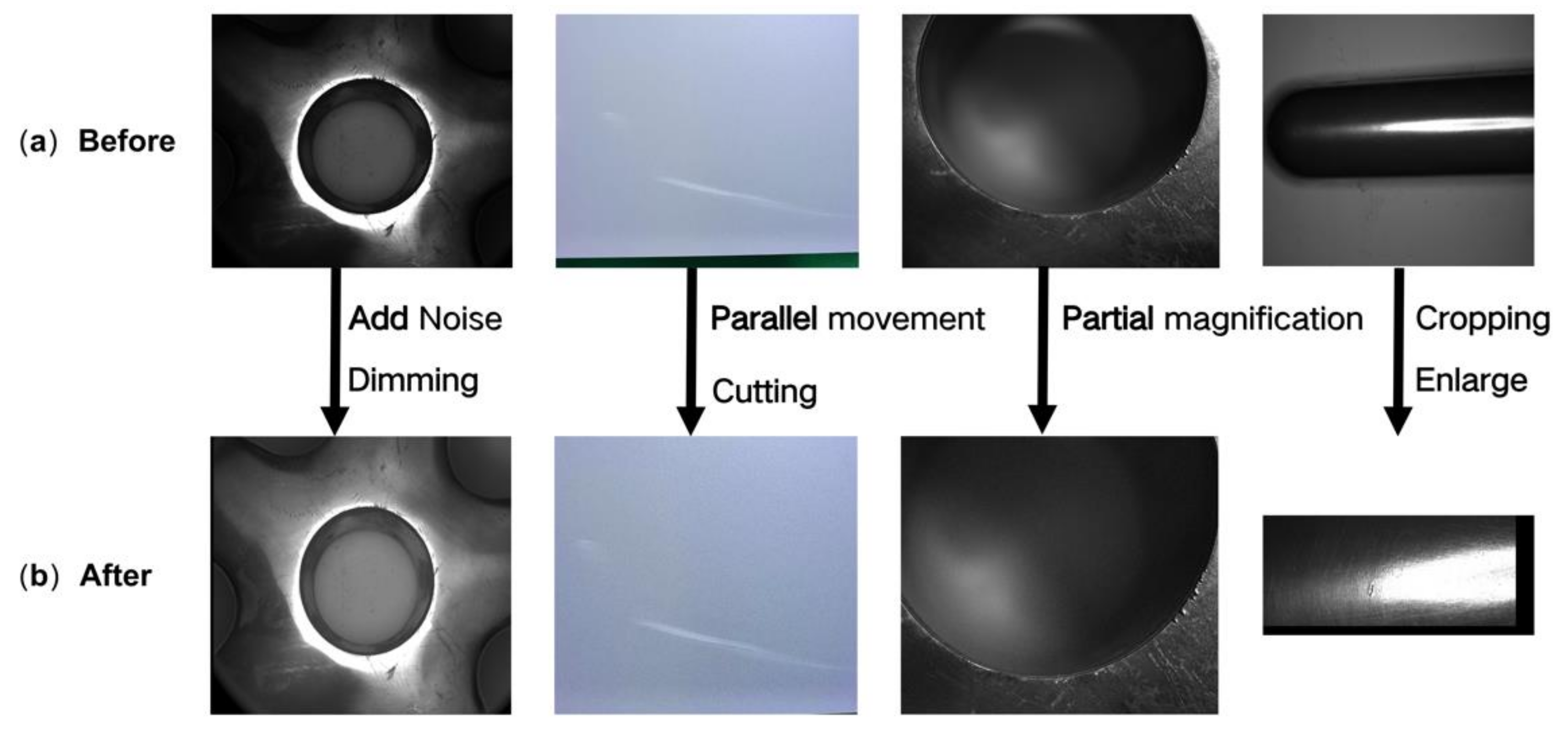
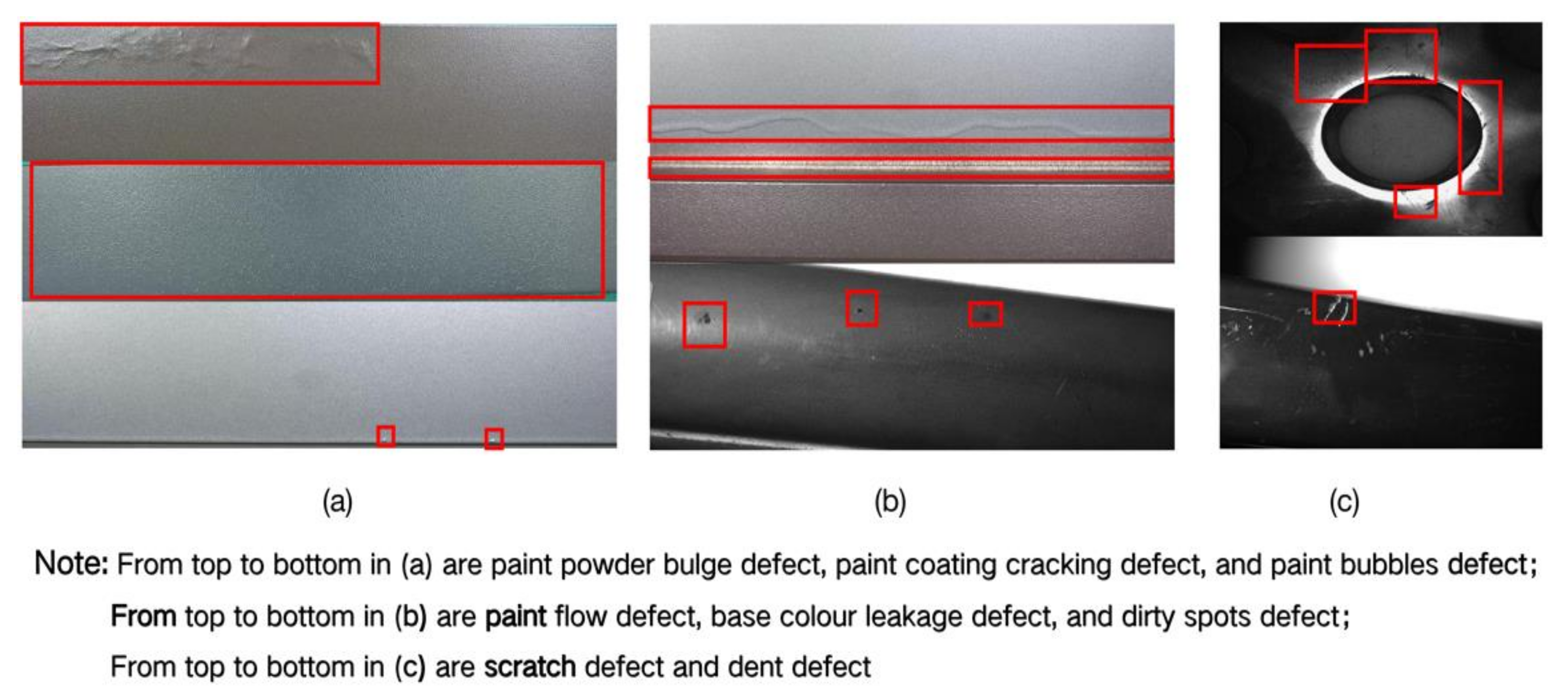
4.1. Experimental Dataset

The five-star feet are a key component of the office chair, which support and stabilize the whole office chair. The five-star feet are shown in Figure 7. At present, the production materials of the five-star feet for the office chair are mainly metal and nylon. The production of the data set in this paper mainly considers the five-star feet made of metal materials.

The data set comes from the five-star feet of office chairs shot by industrial cameras. The self-made data set is augmented and optimized by writing scripts to obtain 2300 images. The processing methods of data set image augmentation mainly include cropping, parallel movement, adding noise, dimming, etc.; the step of cropping is shown in Algorithm 2, and the step of parallel movement is shown in Algorithm 3; the image augmentation processing results of the dataset are shown in Figure 8. Augmented optimization of dataset images can enrich datasets and make dataset images more suitable for training. LabelImg labeling software was used for sample labeling, the data set was in VOC format, and it was divided into a training set, validation set, and test set. Due to the different sizes of the original pictures, the pixels of the pictures are uniformly processed to 416 × 416.

Algorithm 2 Image cropping

Input: W and H are the width and height of the input image. $B_{xmin}$$, B_{xmax}$$, B_{ymin}$ and $B_{ymax}$ are the bounding box information in the input XML file.

Output: new image, new XML file.

1. $x_{max}\leftarrow max\left(0,B_{xmax}\right)$

2. $y_{max}\leftarrow max(0,B_{ymax}$)

3. $x_{min}\leftarrow min\left(W,B_{xmin}\right)$

4. $y_{min}\leftarrow min\left(H,B_{ymin}\right)$

5. $d_r\leftarrow W-x_{max}$

6. $d_b\leftarrow H-y_{max}$

7. $C_{xmin}\leftarrow max\left(0,int\left(x_{min}-random.uniform\left(0,x_{min}\right)\right)\right)$

8. $C_{ymin}\leftarrow max\left(0,int\left(y_{min}-random.uniform\left(0,y_{min}\right)\right)\right)$

9. $C_{xmax}\leftarrow min\left(W,int\left(x_{max}-random.uniform\left(0,d_r\right)\right)\right)$

10. $C_{ymax}\leftarrow min\left(H,int\left(y_{max}-random.uniform\left(0,d_b\right)\right)\right)$

11. crop_img$\leftarrow img\left[C_{ymin}:C_{ymax},C_{xmin} :C_{xmax}\right]$

12. crop_bboxes$\leftarrow \left[B_{xmin}-C_{xmin},B_{ymin}-C_{ymin},B_{xmax}-C_{xmin},B_{ymax}-C_{ymin}\right]$

The process of this algorithm can be understood as follows: First, obtain a set of data according to the input parameters, as shown in the first four steps. Then, calculate the maximum right-shift distance and the maximum down-shift distance, including all target boxes. Steps 7 to 10 are to randomly expand this minimum box and ensure that it does not exceed the bounds. Finally, obtain the cropped image and the information of the cropped bounding box.

Algorithm 3 Image cropping

Input: W and H are the width and height of the input image. $B_{xmin}$$, B_{xmax}$$, B_{ymin}$$\mathrm{and} B_{ymax}$ are the bounding box information in the input XML file.

Output: new image, new XML file.

1. $x_{max}\leftarrow max\left(0,B_{xmax}\right)$

2. $y_{max}\leftarrow max\left(0,B_{ymax}\right)$

3. $x_{min}\leftarrow min\left(W,B_{xmin}\right)$

4. $y_{min}\leftarrow min\left(H,B_{ymin}\right)$

5. $d_r\leftarrow W-x_{max}$

6. $d_b\leftarrow H-y_{max}$

7. $x\leftarrow random.uniform\left(-\frac{x_{min}-1}{3},\frac{d_r-1}{3}\right)$

8. $y\leftarrow random.uniform\left(-\frac{y_{min}-1}{3},\frac{d_b-1}{3}\right)$

9. $M\leftarrow np.float32\left(\left[1,0,x\right],\left[0,1,y\right]\right)$

10. shift_img$\leftarrow cv2.warpAffine\left(img, M, \left(W，H\right)\right)$

11. shift_bboxes$\leftarrow \left[B_{xmin}+x, B_{ymin}+y, B_{xmax}+x, B_{ymax}+y\right]$

The process of this algorithm can be understood as follows: First, obtain a set of data according to the input parameters, as shown in the first four steps. Then, calculate the maximum right-shift distance and the maximum down-shift distance, including all target boxes. In step 7, x is the pixel value moved left or right, positive is right, and negative is left; y is the pixel value moved up or down, positive is up, and negative is down. In step 8, M is an affine transformation matrix, which is used to represent the relation of translation or rotation. Finally, obtain the horizontally shifted image and the information of the horizontally shifted bounding box.

When combined with the actual production, this paper divides the paint surface defects of five-star feet into paint powder bulge defect, paint coating cracking defect, paint bubbles defect, paint flow defect, base color leakage defect, dirty spots defect, scratch defect, dent defect, etc. This article is mainly for the detection of a single defect on the five-star feet. A single defect means that only one type of paint surface defect appears on a picture. As shown in Figure 9, the first column from the left is a paint powder bulge defect, a paint coating cracking defect, and a paint bubbles defect, the second column is a paint flow defect, a base color leakage defect, and a dirty spots defect, and the third column is a scratch defect and a dent defect.

As can be seen from Figure 8, paint bubbles and dirty spots are the main small target defect types in the self-made dataset. Among them, paint bubble defects include defects less than or equal to 5mm, and dirty spot defects include defects less than or equal to 6 mm². The original YOLOv3 algorithm is insufficient for the detection of small target defects. The improved YOLOv3 algorithm proposed in this paper will be applied in the self-made data set to verify the performance of the algorithm.

4.2. Evaluation Indicators

When evaluating the performance of the model, it is usually necessary to take into account both the precision rate and the recall rate. Equation (9) is the formula for calculating the precision rate, and Equation (10) is the formula for calculating the recall rate. The average precision rate under different recall rates is defined as the Average Precision (AP), which is used to evaluate the detection accuracy of a certain class. In target detection, the mean Average Precision (mAP) is usually used to evaluate the model performance, and the small target missed detection rate is evaluated by comparing the prediction effect before and after the YOLOv3 algorithm. The precision and recall are defined as the following equation.

$$precision=\frac{TP}{TP+FP}$$

(9)

$$recall=\frac{TP}{TP+FN}$$

(10)

In Equations (9) and (10), TP is the number of positive samples successfully predicted, FP is the number of negative samples incorrectly predicted as positive samples by the model, and FN is the number of positive samples incorrectly predicted as negative samples by the model.

The precision rate represents the proportion of the number of correctly predicted samples in the prediction target of a certain category to the total number of correct samples, and the recall rate represents the proportion of the number of correctly predicted samples to the total number of predicted samples. In this paper, the performance of the model will be evaluated by using the two indexes of mAP and fps. The calculation Equation of mAP and fps are as follows.

$$mAP=\frac{{{\displaystyle \sum }}_{i=0}^{n}AP\left(i\right)}{n}$$

(11)

$$fps=\frac{Num Figure}{Total Time}$$

(12)

In Equation (11), AP(i) is the detection accuracy of a certain category, and n is the number of categories. In Equation (12), NumFigure is the total number of detected pictures, and TotalTime is the total detection time.

4.3. Analysis of Experimental Results

The hardware configuration of the experimental platform is AMD ryzen7 5800 h Radeon graphics CPU, 16 GB memory, 6 GB NVIDIA GeForce RTX 3060 laptop GPU, the operating system is Windows, and the software environment is CUDA 11.4 and cuDNN V8.2.2. Using PyTorch to build the network model, using the transfer learning idea, loading darknet53.conv.74 as the pre-training weight for training, iterating for a total of 10,000 generations, and the initial configuration parameters (i.e., initial learning rate, number of channels, momentum value, mini-batch size, etc.) have been kept the same as the original parameters in the YOLOv3 model. Figure 10 is the convergence curve of the average loss function during the training process. It can be seen from the figure that the Loss value decreases rapidly at the beginning, and when the iteration approaches 1000 times, the Loss value begins to stabilize.

The experimental results are shown in Figure 11. The first column from the left is a paint powder bulge defect, a paint coating cracking defect, and a paint bubbles defect, the second column is a paint flow defect, a base color leakage defect, and a dirty spots defect, and the third column is a scratch defect and a dent defect. The improved algorithm in this paper achieves an mAP value of 88.3% and a detection speed of 50 f·s⁻¹, which meets the accuracy and real-time requirements for the detection of the paint surface of the five-star feet.

To verify the superiority of the model proposed in this paper, we first compare the detection performance of models using anchor boxes obtained by different clustering algorithms for detection. Secondly, we compare the detection performance of models using different bounding box loss functions. Then, we use the Faster R-CNN algorithm, the SSD algorithm, the YOLOv3 algorithm, and the proposed model to detect the office chair five-star feet paint defect dataset and compare their detection performance. Finally, the proposed model is used to detect defects in the aluminum data set released by the Aliyun Tianchi Competition [24] and compared with the model proposed in the literature [24] to further verify the performance of the proposed model. The test results of the model are based on IOU = 0.5.

• Improve the Network Structure and Clustering Algorithm

Table 2. The average accuracy of the different clustering algorithms.

Network Structure	Clustering Algorithm	fps	mAP@.50 (%)
Original YOLOv3	K-means	55	82.5
Original YOLOv3	K-means||	55	84.2
Proposed model	K-means	50	86.7
Proposed model	K-means++	50	87
Proposed model	K-means||	50	88.3

shows the performance comparison of target detection algorithms after obtaining anchor boxes using different clustering algorithms. After changing the priors anchor clustering method from K-means to K-means||, the mAP value of the original YOLOv3 algorithm has been improved. When using the same clustering algorithm, since the improved YOLOv3 algorithm has been adjusted in the network structure, the mAP value has been significantly improved. When using the same target detection algorithm, the mAP value of K-means|| is better than that of K-means and K-means++. Using the improved YOLOv3 algorithm, combined with the new anchor box clustered by the K-means|| algorithm for defect detection, the mAP value can reach 88.3%.

2.

Comparative Analysis of the Performance of Different Loss Functions

Figure 12 shows the performance comparison of algorithms using different loss functions. It can be seen from Figure 12 that the performance of the algorithm using CIOU is optimized to a certain extent compared to algorithms using other loss functions. In the case of using the original YOLOv3 algorithm, the mAP value using the CIOU loss function is 2.2% higher than that using the IOU loss function. In the case of using the improved YOLOv3 algorithm, the mAP value using the CIOU loss function is 2.7% higher than that using the IOU loss function.

3.

Comparative Analysis of the Performance of Different Algorithms

Table 3. Comparison results of different algorithms.

Algorithm	fps	mAP@.50 (%)
Faster R-CNN	12	79.6
SSD	51	81.3
YOLOv3	55	82.5
Proposed model	50	88.3

shows the performance comparison of different algorithms on the paint surface dataset of self-made office chairs with five-star feet. From the obtained results, it can be found that the mAP value of the improved algorithm in this paper reaches 88.3%, which is better than other comparison algorithms. The detection speed of the improved algorithm in this paper reaches 50$f·s^{-1}$, which is lower than the original algorithm, but it also meets the real-time requirements. The main reason for the reduction in detection speed is that the network structure adds a detection scale, which increases the amount of calculation.

4.

Comparative Analysis of Different Types of Defect Detection Performance

Figure 13 is a comparison of the detection results of the original YOLOv3 algorithm and the improved YOLOv3 algorithm in this paper. The detection scale of the improved YOLOv3 algorithm has been increased from 3 to 4, and 12 a priori anchors need to be set. It can be seen from the results that the mAP values of all defects of the improved YOLOv3 algorithm are improved compared to the original YOLOv3 algorithm. The mAP values for defects such as dirty spots and paint bubbles also increased from 76% and 83% to 81% and 88%, respectively. The improved YOLOv3 algorithm can meet the detection requirements of the five-star feet paint defect types of office chairs in the industry.

5.

Comparative Analysis of Algorithm Performance Based on Public Datasets

We conducted a comparative experiment on the algorithm performance in the Alibaba Tianchi aluminum data set, and the comparison results are shown in

Table 4. Comparison of Algorithms for Aluminum Data Set of the Aliyun Tianchi Competition.

Algorithm	Data Set	fps	mAP @.50 (%)
Improved YOLOv3 [24]	Aliyun Tianchi	51	87.1
Proposed model	Aliyun Tianchi	50	89.2

. The mAP value of the improved algorithm in this paper on the Aliyun Tianchi aluminum data set reaches 89.2%. Compared with the improved algorithm proposed in the literature [24], the mAP value of the improved YOLOv3 algorithm in this paper is also improved.

5. Discussion and Conclusions

We propose an improved YOLOv3 algorithm that can solve the problem of paint defect detection of office chairs’ five-star feet. The clustering algorithm is optimized by using the K-means|| algorithm instead of the traditional K-means algorithm to obtain better anchor boxes. We improve its network structure and loss function to design a fast and accurate end-to-end five-star feet paint defect detection algorithm for office chairs.

The following conclusions are obtained through experiments.

• The new anchor boxes are obtained by K-means|| algorithm clustering, which increases the mAP value by 5.8%.
• By optimizing and improving the network structure of the YOLOv3 algorithm, a new detection scale is added to improve its detection ability for small target defect samples, and the CIOU loss function is used to improve the positioning accuracy. The mAP value is increased by 5.8% compared with the original algorithm.
• On the self-made five-star feet paint surface data set, the mAP value of 8 types of paint surface defect detection reached 88.3%, and the detection speed was also maintained at 50fps. Further verification was carried out on the aluminum data set released by the Aliyun Tianchi Competition. The mAP value of the improved YOLOv3 algorithm in this paper reached 89.2%, and the detection speed could be maintained at 50 fps.
• Through comparative experiments with other algorithms, the improved YOLOv3 algorithm has faster detection speed and better detection accuracy for small target defect detection.

The improved algorithm realizes the end-to-end fast and accurate detection of paint defects on the five-star feet of office chairs.

In this paper, after adding a new detection scale, the overall calculation volume of the algorithm is also increased, which affects the detection speed. Therefore, the network structure can be further optimized in the follow-up research, and the optimizer can be improved to improve the detection performance. At the same time, the preset anchor boxes not only add more parameters to the algorithm but also affect the detection speed. Next, we will further study how to eliminate the dependence on anchor boxes and improve the overall detection speed.

References

1. Chen, C.; Liu, M.-Y.; Tuzel, O.; Xiao, J. R-CNN for small object detection. In Proceedings of the Asian Conference on Computer Vision, Taipei, Taiwan, 20–24 November 2016; pp. 214–230. [Google Scholar]
2. Girshick, R.; Donahue, J.; Darrell, T.; Malik, J. Rich feature hierarchies for accurate object detection and semantic segmentation. In Proceedings of the IEEE Conference on Computer Vision and Pattern Recognition, Columbus, OH, USA, 23–28 June 2014; pp. 580–587. [Google Scholar]
3. Girshick, R. Fast r-cnn. In Proceedings of the IEEE International Conference on Computer Vision, Washington, DC, USA, 7–13 December 2015; pp. 1440–1448. [Google Scholar]
4. Ren, S.; He, K.; Girshick, R.; Sun, J. Faster R-CNN: Towards Real-Time Object Detection with Region Proposal Networks. IEEE Transactions on Pattern Analysis & Machine Intelligence. 2017, 39, 1137–1149. [Google Scholar] [CrossRef] [Green Version]
5. Wang, Y.; Liu, M.; Zheng, P.; Yang, H.; Zou, J. A smart surface inspection system using faster R-CNN in cloud-edge computing environment. Adv. Eng. Inform. 2020, 43, 101037. [Google Scholar] [CrossRef]
6. Tian, Z.; Shen, C.; Chen, H.; He, T. Fcos: Fully convolutional one-stage object detection. In Proceedings of the IEEE/CVF International Conference on Computer Vision, Seoul, Korea, 27–28 October 2019; pp. 9627–9636. [Google Scholar]
7. Liu, W.; Anguelov, D.; Erhan, D.; Szegedy, C.; Reed, S.; Fu, C.-Y.; Berg, A.C. Ssd: Single shot multibox detector. In Proceedings of the European Conference on Computer Vision, Amsterdam, The Netherlands, 11–14 October 2016; pp. 21–37. [Google Scholar]
8. Zhai, S.; Shang, D.; Wang, S.; Dong, S. DF-SSD: An improved SSD object detection algorithm based on DenseNet and feature fusion. IEEE Access 2020, 8, 24344–24357. [Google Scholar] [CrossRef]
9. Qing, Y.; Liu, W.; Feng, L.; Gao, W. Improved Yolo network for free-angle remote sensing target detection. Remote Sens. 2021, 13, 2171. [Google Scholar] [CrossRef]
10. Redmon, J.; Divvala, S.; Girshick, R.; Farhadi, A. You only look once: Unified, real-time object detection. In Proceedings of the IEEE conference on Computer Vision and Pattern Recognition, Las Vegas, NV, USA, 27–30 June 2016; pp. 779–788. [Google Scholar]
11. Redmon, J.; Farhadi, A. YOLO9000: Better, faster, stronger. In Proceedings of the IEEE Conference on Computer Vision and Pattern Recognition, Honolulu, HI, USA, 21–26 July 2017; pp. 7263–7271. [Google Scholar]
12. Cheng, L.; Li, J.; Duan, P.; Wang, M. A small attentional YOLO model for landslide detection from satellite remote sensing images. Landslides 2021, 18, 2751–2765. [Google Scholar] [CrossRef]
13. Liu, C.; Wu, Y.; Liu, J.; Sun, Z. Improved YOLOv3 Network for Insulator Detection in Aerial Images with Diverse Background Interference. Electronics 2021, 10, 771. [Google Scholar] [CrossRef]
14. Redmon, J.; Farhadi, A. Yolov3: An incremental improvement. arXiv 2018, arXiv:1804.02767. [Google Scholar]
15. Tian, Y.; Yang, G.; Wang, Z.; Li, E.; Liang, Z. Detection of apple lesions in orchards based on deep learning methods of cyclegan and yolov3-dense. J. Sens. 2019, 2019, 7630926. [Google Scholar] [CrossRef]
16. Xianbao, C.; Guihua, Q.; Yu, J.; Zhaomin, Z. An improved small object detection method based on Yolo V3. Pattern Anal. Appl. 2021, 24, 1347–1355. [Google Scholar] [CrossRef]
17. Zhao, L.; Li, S. Object detection algorithm based on improved YOLOv3. Electronics 2020, 9, 537. [Google Scholar] [CrossRef] [Green Version]
18. Yu, J.; Zhang, W. Face mask wearing detection algorithm based on improved YOLO-v4. Sensors 2021, 21, 3263. [Google Scholar] [CrossRef] [PubMed]
19. Roy, A.M.; Bhaduri, J. Real-time growth stage detection model for high degree of occultation using DenseNet-fused YOLOv4. Comput. Electron. Agric. 2022, 193, 106694. [Google Scholar] [CrossRef]
20. Roy, A.M.; Bose, R.; Bhaduri, J. A fast accurate fine-grain object detection model based on YOLOv4 deep neural network. Neural Comput. Appl. 2022, 1–27. [Google Scholar] [CrossRef]
21. Nepal, U.; Eslamiat, H. Comparing YOLOv3, YOLOv4 and YOLOv5 for Autonomous Landing Spot Detection in Faulty UAVs. Sensors 2022, 22, 464. [Google Scholar] [CrossRef]
22. Jiang, X.; Gao, T.; Zhu, Z.; Zhao, Y. Real-time face mask detection method based on YOLOv3. Electronics 2021, 10, 837. [Google Scholar] [CrossRef]
23. Rani, E. LittleYOLO-SPP: A delicate real-time vehicle detection algorithm. Optik 2021, 225, 165818. [Google Scholar]
24. Zhang, X.; Huang, D. Defect detection on aluminum surfaces based on deep learning. J. East China Norm. Univ. (Nat. Sci.) 2020, 2020, 105. [Google Scholar]
25. Li, W.; Ye, X.; Zhao, Y.; Wang, W. Strip Steel Surface Defect Detection Based on Improved YOLOv3 Algorithm. Acta Electron. Sin. 2020, 48, 1284–1292. [Google Scholar]
26. Xu, L.; Huang, H.; Ding, W.; Fan, Y. Detection of small fruit target based on improved DenseNet. J. Zhejiang Univ. (Eng. Sci.) 2021, 55, 377–385. [Google Scholar]
27. Rezatofighi, H.; Tsoi, N.; Gwak, J.; Sadeghian, A.; Savarese, S. Generalized Intersection Over Union: A Metric and a Loss for Bounding Box Regression. In Proceedings of the 2019 IEEE/CVF Conference on Computer Vision and Pattern Recognition (CVPR), Long Beach, CA, USA, 15–16 June 2019. [Google Scholar]
28. Zheng, Z.; Wang, P.; Liu, W.; Li, J.; Ye, R.; Ren, D. Distance-IoU loss: Faster and better learning for bounding box regression. In Proceedings of the AAAI Conference on Artificial Intelligence, New York, NY, USA, 7–12 February 2020; pp. 12993–13000. [Google Scholar]
29. Bahmani, B.; Moseley, B.; Vattani, A.; Kumar, R.; Vassilvitskii, S. Scalable k-means++. arXiv 2012, arXiv:1203.6402 2012. [Google Scholar] [CrossRef]
30. Hämäläinen, J.; Kärkkäinen, T.; Rossi, T. Improving scalable K-means++. Algorithms 2021, 14, 6. [Google Scholar] [CrossRef]
Figure 1. YOLOv3 algorithm network structure.
Machines 10 00261 g001
Figure 2. Darknet-53 network structure.
Machines 10 00261 g002
Figure 3. Improved YOLOv3 algorithm network structure.
Machines 10 00261 g003
Figure 4. The relative distance between the bounding boxes.
Machines 10 00261 g004
Figure 5. GIOU and CIOU’s bounding box regression steps. a(green box) and b(black box) denote target box and anchor box, respectively. c(blue box in GIOU, red box in CIOU) denote predicted boxes.
Machines 10 00261 g005
Figure 6. A priori box clustering result.
Machines 10 00261 g006
Figure 7. Five-star feet of the office chair.
Machines 10 00261 g007
Figure 8. Data set image augmentation processing results (partial).
Machines 10 00261 g008
Figure 9. Manually marked defects (partial).
Machines 10 00261 g009
Figure 10. Convergence curve of loss function.
Machines 10 00261 g010
Figure 11. Defects detected and flagged by the proposed model (partial).
Machines 10 00261 g011
Figure 12. Comparison of mAP values obtained using different loss functions.
Machines 10 00261 g012
Figure 13. Comparison of mAP values of different defects.
Machines 10 00261 g013