
Multi-Objective Design Optimization of Flexible Manufacturing Systems Using Design of Simulation Experiments: A Comparative Study

 ,
,  , ,
, ,
Abstract
:1. Introduction
1.1. Literature Overview
1.1.1. General Literature Review of MOSO Methods
- According to the articulation of the preferences of the Decision Maker (DM). This first classification criterion is proposed by Rosen et al. [8]. Four groups of methods are possible and include the following: (1) a priori MOSO methods when the DM expresses their preferences before optimization is conducted; (2) a posteriori MOSO methods (in these methods, the DM selects a solution at the end of the search. Although this approach avoids the disadvantage of the a priori approach by taking into account preference information only at the end of the optimization process, it can lead to extremely high computational costs); (3) a progressive articulation of DM preferences (also named Interactive MOSO Methods) (the progressive approaches repeatedly solicit preference information from the DM to guide the optimization process). These methods enable DM to change his preferences during the optimization process by incorporating knowledge that only becomes available during the search. Interactive methods may be useful when simulation runs are expensive and the DM is readily available to provide input. Finally, the fourth group involves (4) non preference MOSO methods that operate without regard to the preference of DM.
- According to the research set and variables nature. This second classification criterion is proposed by Hunter et al. [7]. Three groups of methods are possible, including the following: (1) MOSO on finite sets, called Multi-Objective Ranking and Selection (MORS); (2) MOSO with integer-ordered decision variables; and (3) MOSO with continuous decision variables. In the context of integer-ordered and continuous decision variables, we focus on methods that provably converge to a local efficient set under natural ordering. Furthermore, these methods of the three groups can also be viewed two groups according to the type of the final solution: global solution versus local solution [7]. The MORS methods provide a global solution, in which simulation replications are usually obtained from every point in the finite feasible set, and the estimated solution is the global estimated best. In addition, metaheuristics methods (named also random search) such as simulated annealing, Genetic Algorithms (GA), Tabu Search (TS), etc., also provide global solutions. Metaheuristics methods are efficient because they appropriately control stochastic error. However, the task is more challenging as it results in a number of solutions with different trade-offs among criteria, also known as Pareto optimal or efficient solutions.
- According to the use or non-use of metamodels. This third classification is proposed implicitly in many research studies such as in Barton and Meckesheimer [9], do Amaral et al. [10], etc. A metamodel or model of the simulation model simplifies the SO in two ways: The metamodel response is deterministic rather than stochastic, and the run times are generally much shorter than the original simulation. The metamodel is used to identify and estimate the relationship between the inputs and outputs of the simulation model, forming a mathematical function that is used to evaluate possible solutions in the optimization process. For example, Hassannayebi et al. [11] highlight that the adoption of metamodel-based SO in industry and service problems has grown due to its potential to reduce the number of simulation rounds necessary in the optimization process. Note that the MOSO methods, which are based on the metamodel, also provide a global solution such as that discussed in the second classification criterion.
1.1.2. FMS Design Literature Review
1.2. The Proposed Conceptual Classification of MOSO for FMS Design
1.3. The Objective of the Case Study
2. Materials and Methods
2.1. Simulation of Possible FMS Designs according to the DoE
2.1.1. The Case Study
- To capture the FMS flexibility effect on its performance, this research adopts different machine LAYOUT (LAYOUT) for the studied FMS. Indeed, Functional Layout (FL) and Cellular Layout (CL) are the two most used machine layouts in FMSs. In FL, functionally similar machines are grouped into departments, and all machines of every department can perform production operations for any incoming part [31]. However, CL is made up of independent manufacturing cells. Each of these cells is made up of different machine types dedicated to the treatment of similar parts grouped into families. In addition, this work aimed also to measure the effect of part Batch Size (BS), part Inter-Arrival Time (IAT), and scheduling RULEs (RULE) on FMS performances (Table 3). The IAT, defined as the difference between the arrival times to the FMS of two consecutive parts, is generally generated by common probabilistic laws. In addition, parts are grouped into batches to reduce the machine’s setup repetitions and transport times between work stations [31]. Furthermore, parts arriving at any work station are made to wait in a queue until the required machine becomes available. Once this required machine is idle, parts must be selected from the waiting queue based on scheduling rules [32,33,34]. As shown in Table 3, each of the considered FMS factors considered is studied with 2 levels.
- The FMS considered is composed of 8 machines grouped into 3 departments in FL and 2 cells in CL. The two departments “M” and “L” are composed of 3 machines each, while department “M” comprises only 2 machines. This MS is also characterized by two-part families composed of each of 2 part types. Each type of part requires 2 to 5 manufacturing operations (Table 4).
- The setup and processing times for each type of part are provided in Table 5. Setup times on every machine can be reduced or cancelled by the setup factor (δ) depending on the similarity of the successive parts family or type. Indeed, if successive parts belong to the same family, the subsequent part setup time must be reduced by a factor of δ = 0.5. On the other hand, if these successive parts have the same type, no machine setup is needed and the subsequent part setup time must be cancelled by a factor of δ = 0. Transfer times in the two layouts follow a statistical uniform law between 10 and 16 min.
- To characterize the fluidity of parts flow in FMS, different optimization studies used WIP and MFT as major performance measures [31]. WIP has mainly been measured as the number of parts in the system, and MFT is simply obtained by averaging all durations between every part exit times and entry times in FMS. The TR of the production was adopted as the third performance measure. To evaluate TR, it is normal to measure the number of processed parts per unit of time. The maximization of such a measure of performance reflects the best use of material and human resources. To enhance the efficiency of FMS piloting, various optimization studies used the waiting and transfer times (WT and TT) as performance indicators, and they essentially aimed to minimize these two indicators.
2.1.2. The Simulation Model
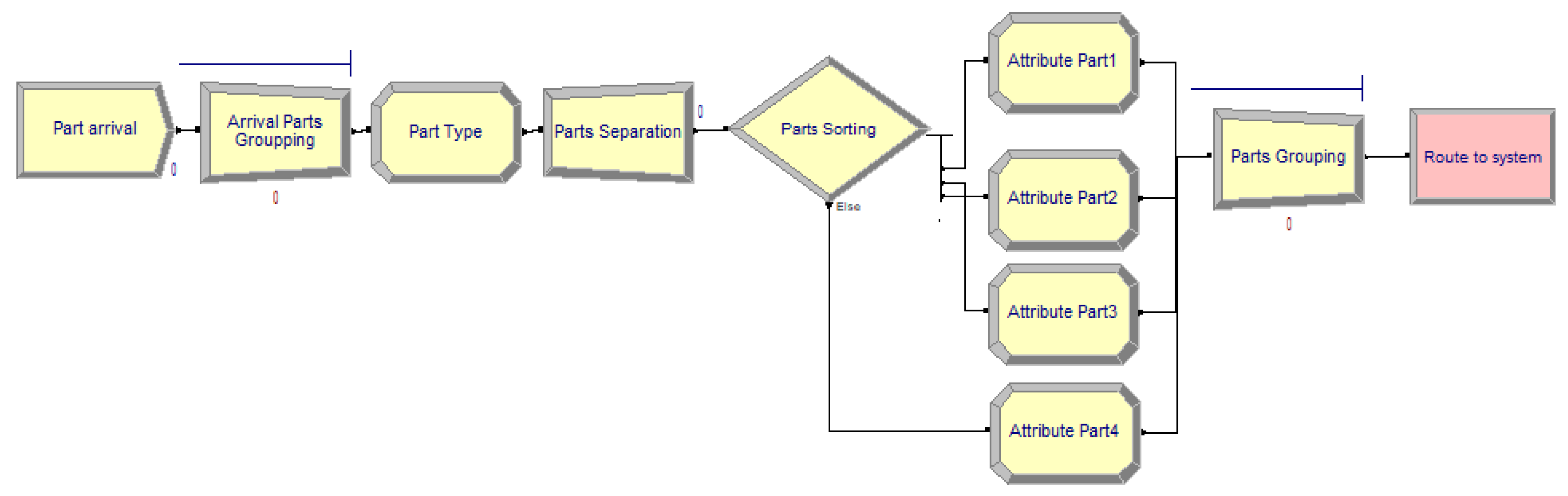
- Parts enter to the system through a “Create” module named “Parts Arrival” in which the BS and IAT times are specified. Then, they are grouped into batches by a “Batch” module, named “Arrival Parts Grouping”, to assign them their corresponding types through an “Assign” module named “Part Type”. Due to the stochastic nature of their PT and ST, these batches are separated into unit products through a “Separate” module called “Parts Separation” to assign them each of their execution times through one of the four “Assign” modules named “Attribute Part i’’. However, a preliminary step must be performed through a “Decide” module called “Parts Sorting” to direct each type of product to the corresponding “Assign” module. The products then proceed through a “Batch” module named “Parts Grouping” before proceeding through the “Route” module named “Transfer to System’’ (Figure 2).
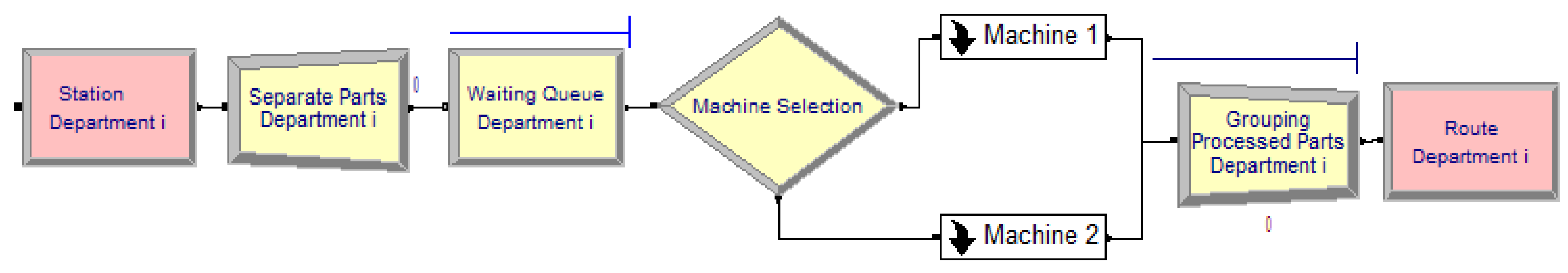
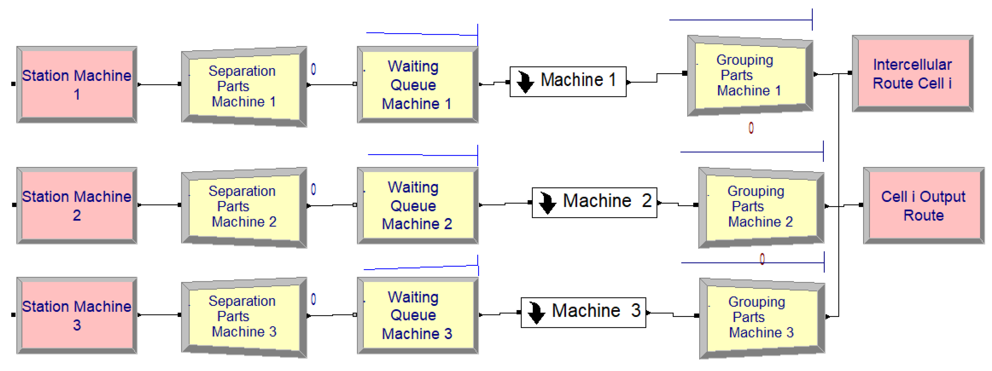
- As soon as one products batch arrives in one of the departments, it is separated into unit products and put on hold in the department queue via the “Hold” module named “Waiting Queue Department i”. This queue is governed by a “Queue” module in which the scheduling rule must be specified. Once one of the department machines becomes free, the selected waiting product is released from the “Hold” module. It then passes through a test, represented by the module “Decide” named “Machine Selection”, which affects it toward this free machine. The processed products of the machines are grouped again in batches by the “Batch” module named “Grouping of Processed Parts Department i’’, which succeeds these machines. Finally, each batch of products is transferred to the next step in its production sequence through the module called “Route Department i’’ (Figure 3).


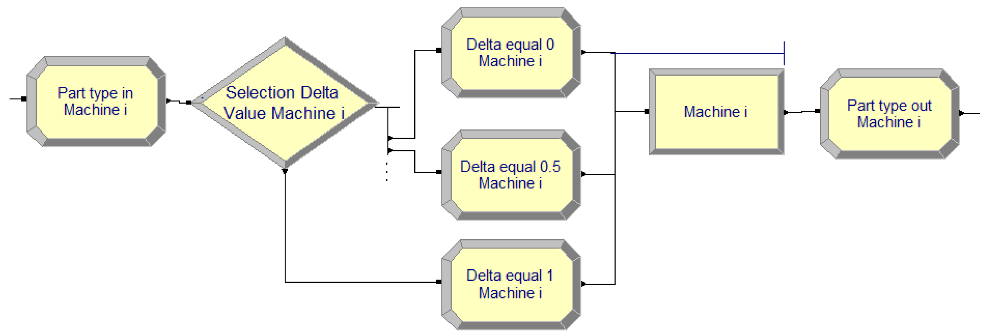
- In the two FL and CL simulation models, the machines are modeled by “Process” modules. In these modules, the transformation times are defined, which are function of PT and ST weighted by factor δ. Thus, Transformation time = PT + δxST. The value of factor δ depends on the similarity of the types of products entering and leaving the machine. In fact, a module called “Selection Delta Value Machine Selection i” applies a test on all incoming products to the machine to look for the value of this factor. For this, it compares two variables named “Part Type” and “Part Family” defined in the two “Assign” modules, named “Part Type in Machine i” and “Part Type Out Machine i”. If the two variables “Part Type” are identical, the module “Delta value machine selection i” directs the incoming product to the module “Assign” named “Delta Equal 0 Machine i” corresponding to the value of factor δ = 0. If the two variables “Part Type” are different but the two variables “Part Family” are identical, the module “Delta Value Machine i” directs the incoming product to the module “Assign” named “Delta Equal 0.5 Machine i” corresponding to the value of factor δ = 0.5. Otherwise, module “Selection Delta Value Selection Machine i” directs the incoming product to the module “Assign” named “Delta Equal 1 Machine i”, corresponding to the value of factor δ = 1 (Figure 5).
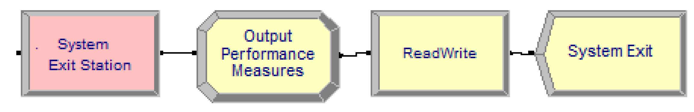
- The leaving products batch proceeds through an “Assig” module, called “Output Performance Measures”, for computing and updating all variables defined as performance measures. The acquired data are then stored in an Excel file using a “Readwrite” module for further treatment and analysis. Finally, the batches of products are evacuated from the simulation model via the “Dispose” module named “System Exit” (Figure 6).
2.2. Design of Experiments (DoE)
2.3. Multi-Objective Optimization Methods
2.3.1. The GP Method
- gi: The goal set for the ith objective for (i =1…p) (the objectives here are the performance measures);
- xj: The jth decision variable for (j = 1…n) (the decision variables here are the significant FMS factors and interactions);
- aij: The technological parameters (these parameters are the coefficients of the developed mathematical models relating the performance measures to significant FMS factors and interactions);
- : The matrix of coefficients related to the physical FMS constraints;
- C: The vector of available physical FMS resources;
- The positive and negative deviations from the goals values.
2.3.2. The DF Method
2.3.3. The GRA Method
2.3.4. The VIKOR Method
3. Results
3.1. Simulation Results
3.2. Multi-Objective Optimization Methods
3.2.1. The GP Method
- Determination of statistically significant FMS parameters: The main effects of the studied factors and interactions were analyzed in α = 0.05 of significance levels using the MINITAB statistical package (Table 6). Significant factors and interactions (p ≤ 0.05) are shown in bold.
- 2.
- Development of mathematical models: Based on the simulation results, mathematical models were computed. Regression Equations (27)–(31) with identified significant factors and interactions effects have been derived for MFT, WIP, TT, and WT.
| MFT = 144.633 – 13633 × BS − 5742.6 × IAT − 68028 × RULE − 71627 × LAYOUT + 542.4 × BS × IAT + 6511 × BS × RULE + 6809 × BS × LAYOUT + 2721.8 × IAT × RULE + 2845.2 × IAT × LAYOUT + 33807 × RULE × LAYOUT − 260.52 × BS × IAT × RULE − 269.48 × BS × IAT × LAYOUT − 3235.7 × BS × RULE × LAYOUT − 1352.5 × IAT × RULE × LAYOUT + 129.46 × BS × IAT × RULE × LAYOUT | (27) |
| With R2 = 99.41% and R2(adj) = 99.34%, |
| WIP = 1078.3 − 96.84 × BS − 42.75 × IAT + 239.6 × RULE − 529.2 × LAYOUT + 3.849 × BS × IAT − 25.91 × BS × RULE + 48.47 × BS × LAYOUT − 9.52 × IAT × RULE + 20.99 × IAT × LAYOUT − 121.6 × RULE × LAYOUT + 1.031 × BS × IAT × RULE − 1.912 × BS × IAT × LAYOUT + 13.16 × BS × RULE × LAYOUT + 4.835 × IAT × RULE × LAYOUT − 0.5237 × BS × IAT × RULE × LAYOUT | (28) |
| With R2 = 99.47% and R2(adj) = 99.42%, |
| TP = −61.61 + 9.883 × BS + 4.1508 × IAT + 2.415 × RULE + 98.713 × LAYOUT − 0.50632 × BS × IAT − 9.4912 × BS × LAYOUT − 0.0971 × IAT × RULE − 3.9333 × IAT × LAYOUT − 1.116 × RULE × LAYOUT + 0.37771 × BS × IAT × LAYOUT + 0.0448 × IAT × RULE × LAYOUT | (29) |
| With R2 = 99.88% and R2(adj) = 99.87%, |
| TT = 3.12 + 51.558 × BS − 1.898 × LAYOUT − 12.7192 × BS × LAYOUT | (30) |
| With R2 = 99.97% and R2(adj) = 99.97%, |
| WT = 669,420 − 58944 × BS − 26657 × IAT − 298872 × RULE − 334431 × LAYOUT + 2351 × BS × IAT + 27062 × BS × RULE + 30009 × BS × LAYOUT + 11951 × IAT × RULE + 13247 × IAT × LAYOUT + 148498 × RULE × LAYOUT − 1081.9 × BS × IAT × RULE − 1176.1 × BS × IAT × LAYOUT − 13447 × BS × RULE × LAYOUT − 5937 × IAT × RULE × LAYOUT + 537.4 × BS × IAT × RULE × LAYOUT | (31) |
| With R2 = 97.86% and R2(adj) = 97.64%, |
- 3.
- GP model formulation and resolution: We propose a GP model in which the selected performance measures are considered. The optimal configuration of decision variables minimizes the sum of penalties (dj). The parameter dj are deviations from the desired levels of the goals that are subject to series constraints. With the regression equations presented previously, the above-mentioned goal programming model can be stated as shown in Equations (32)–(40):
| (33) | |
| (34) | |
| (35) | |
| (36) | |
| (37) | |
| LAYOUT and RULE are binary (1 or 2), | (38) |
| 5 ≤ IAT ≤ 25, | (39) |
| 5 ≤ BS ≤ 10, | (40) |
- 4.
- The GP model was solved using the mathematical software LINGO 18.0. The best value of the objective function was found to be equal to 136.99 and was obtained for the following levels of the studied factors: LAYOUT = CL, RULE = FCFS, IAT = 25, and BS = 5.
3.2.2. The DF Method
3.2.3. The GRA Method
3.2.4. The VIKOR Method
4. Discussion
5. Conclusions
- In this study, four MOSO methods are compared. Two methods belong to group A of the proposed new classification, while the other two belong to group B. The extension of the current comparison to other MOSO methods belonging to group C is the first objective of our interesting perspectives.
- The studied MOSO methods have been applied on a model of an FMS inspired from the literature. This model has six machines grouped in two cells in the CL and three departments in FL. In addition, this FMS processes only four products grouped into two families. Extending the comparison performed in this study to real and more complex FMSs to evaluate the reliability of MOSO methods is the second objective of our interesting perspectives.
- The experimental design developed in this comparison study and which is the basis for the simulation results used in the analysis and generation of optimization solutions is based on four factors: IAT, BS, RULE, and LAYOUT. These four factors are explored on the basis of two levels each. This number of factors and levels remains relatively limited and generates a limited number of experiments. The comparison of MOSO Methods in Manufacturing Systems characterized by a large number of factors and levels is the third objective of our interesting perspectives.
- The application of the compared MOSO methods proceeds through different steps to generate optimization solutions. These steps usually require the intervention of a user to transfer the results from one step to another. The integration of these analysis and optimization steps into the simulation software, as in the case of the OptQuest tool in several simulation tools, would be a very interesting perspective.
Author Contributions
Funding
Institutional Review Board Statement
Informed Consent Statement
Data Availability Statement
Acknowledgments
Conflicts of Interest
Appendix A

| EXP | Factor Levels | Replication | ||||||||||||
|---|---|---|---|---|---|---|---|---|---|---|---|---|---|---|
| LAYOUT | RULE | IAT | BS | 1 | 2 | 3 | 4 | 5 | 6 | 7 | 8 | 9 | 10 | |
| 1 | 1 | 1 | 5 | 5 | 16,334.1 | 16,645.9 | 16,612.2 | 16,866.2 | 17,446.5 | 16,523.3 | 16,778.2 | 16,601.8 | 17,529.3 | 18,119.7 |
| 2 | 1 | 1 | 5 | 10 | 2312.8 | 1636.8 | 2435.7 | 3132.7 | 2374.0 | 3222.1 | 3128.3 | 1968.7 | 4831.2 | 2432.0 |
| 3 | 1 | 1 | 25 | 5 | 597.0 | 549.5 | 559.6 | 528.5 | 614.4 | 540.6 | 583.7 | 577.4 | 552.6 | 569.8 |
| 4 | 1 | 1 | 25 | 10 | 538.0 | 565.0 | 560.4 | 577.7 | 559.5 | 581.1 | 546.9 | 538.7 | 538.2 | 547.6 |
| 5 | 1 | 2 | 5 | 5 | 2574.7 | 3339.8 | 2014.4 | 2735.9 | 2348.5 | 2484.6 | 2698.9 | 1959.8 | 2784.8 | 3760.3 |
| 6 | 1 | 2 | 5 | 10 | 1881.7 | 1261.2 | 1463.6 | 1614.9 | 1166.6 | 1919.4 | 1276.1 | 1449.3 | 1662.2 | 2019.3 |
| 7 | 1 | 2 | 25 | 5 | 547.0 | 570.4 | 567.4 | 564.8 | 552.6 | 559.2 | 599.0 | 565.1 | 606.4 | 577.2 |
| 8 | 1 | 2 | 25 | 10 | 546.7 | 544.0 | 545.1 | 561.6 | 544.9 | 565.4 | 543.0 | 558.3 | 559.2 | 562.0 |
| 9 | 2 | 1 | 5 | 5 | 1460.9 | 1149.0 | 1314.0 | 711.9 | 825.9 | 699.7 | 848.5 | 846.1 | 832.2 | 859.4 |
| 10 | 2 | 1 | 5 | 10 | 1087.7 | 1052.0 | 1305.7 | 993.0 | 1214.9 | 1155.9 | 1038.4 | 1132.8 | 1153.9 | 1085.4 |
| 11 | 2 | 1 | 25 | 5 | 434.5 | 431.8 | 423.1 | 422.7 | 419.7 | 427.9 | 423.9 | 423.9 | 424.8 | 433.5 |
| 12 | 2 | 1 | 25 | 10 | 773.0 | 769.2 | 796.1 | 783.9 | 771.2 | 768.1 | 772.8 | 769.6 | 791.4 | 783.7 |
| 13 | 2 | 2 | 5 | 5 | 690.2 | 717.1 | 752.2 | 721.7 | 1260.2 | 741.1 | 721.4 | 748.1 | 690.2 | 777.0 |
| 14 | 2 | 2 | 5 | 10 | 1159.5 | 1053.5 | 1133.9 | 1121.7 | 1080.1 | 1187.4 | 1071.3 | 1085.1 | 1080.9 | 1094.4 |
| 15 | 2 | 2 | 25 | 5 | 438.0 | 427.5 | 421.1 | 422.6 | 428.0 | 425.6 | 423.8 | 426.3 | 436.3 | 432.3 |
| 16 | 2 | 2 | 25 | 10 | 773.0 | 769.0 | 796.1 | 783.9 | 771.0 | 768.1 | 772.8 | 769.6 | 791.4 | 783.4 |
| EXP | Factor Levels | Replication | ||||||||||||
|---|---|---|---|---|---|---|---|---|---|---|---|---|---|---|
| LAYOUT | RULE | IAT | BS | 1 | 2 | 3 | 4 | 5 | 6 | 7 | 8 | 9 | 10 | |
| 1 | 1 | 1 | 5 | 5 | 276.4 | 285.9 | 287.2 | 288.6 | 296.7 | 286.0 | 286.4 | 288.0 | 299.9 | 308.5 |
| 2 | 1 | 1 | 5 | 10 | 38.5 | 27.3 | 41.1 | 52.3 | 39.8 | 53.7 | 52.1 | 33.1 | 80.0 | 40.6 |
| 3 | 1 | 1 | 25 | 5 | 6.1 | 5.6 | 5.7 | 5.4 | 6.2 | 5.5 | 5.9 | 5.9 | 5.6 | 5.8 |
| 4 | 1 | 1 | 25 | 10 | 5.4 | 5.7 | 5.6 | 5.8 | 5.6 | 5.9 | 5.5 | 5.4 | 5.4 | 5.5 |
| 5 | 1 | 2 | 5 | 5 | 325.0 | 345.3 | 302.0 | 349.1 | 318.0 | 322.5 | 332.9 | 329.0 | 371.0 | 343.7 |
| 6 | 1 | 2 | 5 | 10 | 58.2 | 23.5 | 38.3 | 29.4 | 22.4 | 65.8 | 22.7 | 35.2 | 48.4 | 38.5 |
| 7 | 1 | 2 | 25 | 5 | 5.9 | 6.2 | 6.2 | 6.1 | 6.0 | 6.0 | 6.5 | 6.1 | 6.6 | 6.3 |
| 8 | 1 | 2 | 25 | 10 | 5.6 | 5.6 | 5.6 | 5.7 | 5.6 | 5.8 | 5.5 | 5.7 | 5.7 | 5.7 |
| 9 | 2 | 1 | 5 | 5 | 24.4 | 19.2 | 22.0 | 12.0 | 13.9 | 11.7 | 14.2 | 14.2 | 14.0 | 14.4 |
| 10 | 2 | 1 | 5 | 10 | 18.2 | 17.6 | 21.9 | 16.6 | 20.3 | 19.3 | 17.4 | 18.9 | 19.3 | 18.1 |
| 11 | 2 | 1 | 25 | 5 | 4.4 | 4.4 | 4.3 | 4.3 | 4.3 | 4.3 | 4.3 | 4.3 | 4.3 | 4.4 |
| 12 | 2 | 1 | 25 | 10 | 7.8 | 7.7 | 8.0 | 7.9 | 7.7 | 7.7 | 7.8 | 7.7 | 8.0 | 7.9 |
| 13 | 2 | 2 | 5 | 5 | 14.4 | 13.1 | 14.2 | 13.2 | 24.0 | 13.6 | 16.3 | 13.7 | 12.5 | 13.0 |
| 14 | 2 | 2 | 5 | 10 | 20.1 | 18.1 | 19.7 | 19.4 | 18.6 | 20.6 | 19.1 | 18.7 | 18.7 | 18.8 |
| 15 | 2 | 2 | 25 | 5 | 4.5 | 4.4 | 4.3 | 4.3 | 4.4 | 4.4 | 4.4 | 4.4 | 4.5 | 4.5 |
| 16 | 2 | 2 | 25 | 10 | 7.8 | 7.8 | 8.0 | 7.9 | 7.8 | 7.8 | 7.8 | 7.8 | 8.0 | 7.9 |
| EXP | Factor Levels | Replication | ||||||||||||
|---|---|---|---|---|---|---|---|---|---|---|---|---|---|---|
| LAYOUT | RULE | IAT | BS | 1 | 2 | 3 | 4 | 5 | 6 | 7 | 8 | 9 | 10 | |
| 1 | 1 | 1 | 5 | 5 | 39.54 | 38.37 | 37.72 | 38.23 | 37.29 | 37.99 | 38.23 | 37.76 | 36.74 | 35.8 |
| 2 | 1 | 1 | 5 | 10 | 37.84 | 38.59 | 36.66 | 36.33 | 38.07 | 35.98 | 35.96 | 37.22 | 34.69 | 37.81 |
| 3 | 1 | 1 | 25 | 5 | 28.52 | 28.46 | 28.31 | 28.48 | 28.4 | 28.36 | 28.42 | 28.37 | 28.46 | 28.45 |
| 4 | 1 | 1 | 25 | 10 | 14.31 | 14.31 | 14.31 | 14.26 | 14.31 | 14.26 | 14.31 | 14.28 | 14.24 | 14.27 |
| 5 | 1 | 2 | 5 | 5 | 39.7 | 39.05 | 41.83 | 37.92 | 40.49 | 40.27 | 39.34 | 39.88 | 35.48 | 38.14 |
| 6 | 1 | 2 | 5 | 10 | 36.3 | 38.67 | 37.49 | 38.27 | 38.46 | 35.59 | 39.18 | 37.21 | 36.57 | 37.71 |
| 7 | 1 | 2 | 25 | 5 | 28.52 | 28.48 | 28.35 | 28.36 | 28.41 | 28.45 | 28.37 | 28.41 | 28.33 | 28.28 |
| 8 | 1 | 2 | 25 | 10 | 14.27 | 14.31 | 14.27 | 14.3 | 14.27 | 14.34 | 14.31 | 14.35 | 14.27 | 14.27 |
| 9 | 2 | 1 | 5 | 5 | 76.95 | 77.61 | 77.27 | 78.35 | 78.27 | 78.71 | 78.5 | 78.53 | 78.23 | 78.24 |
| 10 | 2 | 1 | 5 | 10 | 38.79 | 38.88 | 38.56 | 39.05 | 38.91 | 38.88 | 38.89 | 38.91 | 38.87 | 39.12 |
| 11 | 2 | 1 | 25 | 5 | 28.54 | 28.5 | 28.58 | 28.54 | 28.58 | 28.5 | 28.62 | 28.54 | 28.58 | 28.62 |
| 12 | 2 | 1 | 25 | 10 | 14.19 | 14.19 | 14.15 | 14.23 | 14.22 | 14.16 | 14.18 | 14.23 | 14.18 | 14.22 |
| 13 | 2 | 2 | 5 | 5 | 78.5 | 78.52 | 78.24 | 78.47 | 77.5 | 78.6 | 77.39 | 78.63 | 78.72 | 78.46 |
| 14 | 2 | 2 | 5 | 10 | 38.92 | 39.06 | 38.73 | 39.03 | 38.92 | 38.97 | 38.77 | 39.03 | 38.93 | 39.05 |
| 15 | 2 | 2 | 25 | 5 | 28.53 | 28.5 | 28.58 | 28.5 | 28.54 | 28.55 | 28.62 | 28.54 | 28.57 | 28.58 |
| 16 | 2 | 2 | 25 | 10 | 14.19 | 14.19 | 14.15 | 14.23 | 14.22 | 14.16 | 14.18 | 14.23 | 14.18 | 14.22 |
| EXP | Factor Levels | Replication | ||||||||||||
|---|---|---|---|---|---|---|---|---|---|---|---|---|---|---|
| LAYOUT | RULE | IAT | BS | 1 | 2 | 3 | 4 | 5 | 6 | 7 | 8 | 9 | 10 | |
| 1 | 1 | 1 | 5 | 5 | 82,836.8 | 85,752.2 | 86,140.3 | 86,578.0 | 89,250.2 | 84,996.3 | 85,347.6 | 85,214.9 | 89,138.4 | 92,596.2 |
| 2 | 1 | 1 | 5 | 10 | 21,801.7 | 15,089.4 | 22,715.8 | 29,844.8 | 22,789.5 | 30,417.2 | 29,423.0 | 18,018.8 | 46,237.5 | 23,032.6 |
| 3 | 1 | 1 | 25 | 5 | 1927.4 | 1838.2 | 1837.4 | 1681.1 | 2073.2 | 1759.2 | 1939.3 | 1923.3 | 1779.0 | 1920.5 |
| 4 | 1 | 1 | 25 | 10 | 3938.8 | 4089.8 | 4115.0 | 4115.8 | 4030.9 | 4087.6 | 3949.3 | 3991.3 | 4038.8 | 3955.6 |
| 5 | 1 | 2 | 5 | 5 | 26,779.8 | 25,064.3 | 14,124.1 | 24,226.4 | 13,939.3 | 19,553.4 | 21,059.2 | 12,639.7 | 14,090.3 | 37,979.1 |
| 6 | 1 | 2 | 5 | 10 | 17,439.0 | 11,361.6 | 13,119.9 | 15,247.0 | 10,391.8 | 19,065.1 | 11,499.0 | 13,196.1 | 15,287.0 | 19,011.7 |
| 7 | 1 | 2 | 25 | 5 | 1776.7 | 1854.7 | 1843.8 | 1829.6 | 1754.0 | 1829.4 | 1942.5 | 1837.2 | 2073.1 | 1883.9 |
| 8 | 1 | 2 | 25 | 10 | 4019.1 | 4010.4 | 4017.5 | 4086.7 | 4034.9 | 4129.1 | 3973.3 | 4076.8 | 4030.6 | 4063.8 |
| 9 | 2 | 1 | 5 | 5 | 6628.1 | 5230.5 | 5937.7 | 3069.7 | 3627.5 | 3008.1 | 3746.4 | 3740.8 | 3663.6 | 3781.3 |
| 10 | 2 | 1 | 5 | 10 | 10,025.4 | 9574.9 | 12,052.1 | 8981.6 | 11,220.2 | 10,425.2 | 9458.4 | 10,387.8 | 10,438.4 | 9835.0 |
| 11 | 2 | 1 | 25 | 5 | 1664.4 | 1655.0 | 1637.7 | 1637.6 | 1634.2 | 1676.7 | 1646.6 | 1630.7 | 1640.7 | 1653.1 |
| 12 | 2 | 1 | 25 | 10 | 6773.5 | 6798.3 | 6731.1 | 6853.6 | 6657.2 | 6739.5 | 6990.0 | 6786.5 | 6747.4 | 6830.7 |
| 13 | 2 | 2 | 5 | 5 | 3367.2 | 3093.6 | 3233.1 | 3102.4 | 5799.1 | 3205.1 | 3084.3 | 3216.5 | 3006.0 | 3062.0 |
| 14 | 2 | 2 | 5 | 10 | 10,596.6 | 9474.9 | 10,320.7 | 10,257.9 | 9831.7 | 10,804.9 | 9753.2 | 9931.9 | 9828.1 | 9990.0 |
| 15 | 2 | 2 | 25 | 5 | 1671.3 | 1631.5 | 1636.3 | 1632.5 | 1646.6 | 1654.3 | 1646.3 | 1651.4 | 1693.2 | 1689.2 |
| 16 | 2 | 2 | 25 | 10 | 6772.9 | 6796.7 | 6730.7 | 6853.6 | 6654.9 | 6739.5 | 6707.0 | 6786.5 | 6747.4 | 6827.4 |
| EXP | Factor Levels | Replication | ||||||||||||
|---|---|---|---|---|---|---|---|---|---|---|---|---|---|---|
| LAYOUT | RULE | IAT | BS | 1 | 2 | 3 | 4 | 5 | 6 | 7 | 8 | 9 | 10 | |
| 1 | 1 | 1 | 5 | 5 | 194.0 | 194.6 | 195.2 | 195.2 | 196.3 | 194.5 | 195.0 | 195.2 | 195.6 | 194.2 |
| 2 | 1 | 1 | 5 | 10 | 389.9 | 389.1 | 390.2 | 389.2 | 387.4 | 389.8 | 389.4 | 389.2 | 390.6 | 388.4 |
| 3 | 1 | 1 | 25 | 5 | 194.7 | 195.4 | 195.0 | 194.7 | 195.7 | 195.5 | 195.4 | 194.9 | 194.7 | 194.1 |
| 4 | 1 | 1 | 25 | 10 | 388.3 | 389.2 | 388.9 | 390.1 | 389.0 | 389.7 | 390.0 | 389.6 | 386.9 | 388.8 |
| 5 | 1 | 2 | 5 | 5 | 195.7 | 195.2 | 194.6 | 197.1 | 193.3 | 193.9 | 195.2 | 210.8 | 194.0 | 194.4 |
| 6 | 1 | 2 | 5 | 10 | 392.3 | 387.7 | 390.0 | 388.1 | 390.3 | 392.1 | 389.9 | 390.8 | 390.7 | 389.5 |
| 7 | 1 | 2 | 25 | 5 | 195.5 | 194.8 | 195.1 | 195.9 | 195.2 | 195.4 | 194.9 | 195.3 | 195.3 | 195.5 |
| 8 | 1 | 2 | 25 | 10 | 391.7 | 388.7 | 390.9 | 389.4 | 389.7 | 390.2 | 388.3 | 387.6 | 392.7 | 390.1 |
| 9 | 2 | 1 | 5 | 5 | 130.0 | 130.1 | 130.3 | 130.4 | 129.9 | 129.9 | 129.7 | 130.7 | 129.7 | 130.3 |
| 10 | 2 | 1 | 5 | 10 | 262.1 | 259.5 | 261.0 | 260.6 | 260.6 | 259.9 | 258.8 | 261.0 | 260.5 | 259.6 |
| 11 | 2 | 1 | 25 | 5 | 130.2 | 129.0 | 130.2 | 130.5 | 129.4 | 130.1 | 129.2 | 130.3 | 129.6 | 130.4 |
| 12 | 2 | 1 | 25 | 10 | 258.4 | 258.8 | 261.2 | 259.6 | 261.2 | 260.4 | 261.0 | 259.3 | 262.8 | 260.4 |
| 13 | 2 | 2 | 5 | 5 | 129.4 | 129.7 | 129.8 | 129.9 | 129.8 | 130.4 | 130.1 | 129.9 | 130.3 | 129.9 |
| 14 | 2 | 2 | 5 | 10 | 262.6 | 260.9 | 259.8 | 261.4 | 260.5 | 261.7 | 260.1 | 260.8 | 262.4 | 260.7 |
| 15 | 2 | 2 | 25 | 5 | 130.0 | 128.9 | 130.0 | 130.2 | 130.0 | 129.9 | 129.2 | 129.9 | 129.4 | 130.2 |
| 16 | 2 | 2 | 25 | 10 | 258.4 | 258.8 | 261.2 | 259.6 | 261.2 | 260.4 | 261.0 | 259.3 | 262.8 | 260.4 |
References
- Salah, B.; Alsamhan, A.M.; Khan, S.; Ruzayqat, M. Designing and Developing a Smart Yogurt Filling Machine in the Industry 4.0 Era. Machines 2021, 9, 300. [Google Scholar] [CrossRef]
- Mian, S.H.; Salah, B.; Ameen, W.; Moiduddin, K.; Alkhalefah, H. Adapting Universities for Sustainability Education in Industry 4.0: Channel of Challenges and Opportunities. Sustainability 2020, 12, 6100. [Google Scholar] [CrossRef]
- Florescu, A.; Barabas, S.A. Modeling and Simulation of a Flexible Manufacturing System—A Basic Component of Industry 4.0. Appl. Sci. 2020, 10, 8300. [Google Scholar] [CrossRef]
- Saren, S.K.; Tiberiu, V. Review of flexible manufacturing system based on modeling and simulation. Fascicle Manag. Technol. Eng. 2016, 24, 113–118. [Google Scholar] [CrossRef]
- Ammeri, A.; Hachicha, W.; Chabchoub, H.; Masmoudi, F. A comprehensive literature review of mono-objective simulation optimization methods. Adv. Prod. Eng. Manag. 2011, 6, 291–302. [Google Scholar]
- Hachicha, W. A Simulation Metamodeling based Neural Networks for Lot-sizing problem in MTO sector. Int. J. Simul. Model. 2011, 10, 191–203. [Google Scholar] [CrossRef]
- Hunter, S.R.; Applegate, E.A.; Arora, V.; Chong, B.; Cooper, K.; Rincón-Guevara, O.; Vivas-Valencia, C. An Introduction to Multiobjective Simulation Optimization. ACM Trans. Modeling Comput. Simul. 2019, 29, 1–36. [Google Scholar] [CrossRef]
- Rosen, L.; Harmonosky, C.M.; Traband, M.T. Optimization of systems with multiple performance measures via simulation: Survey and recommendations. Comput. Ind. Eng. 2008, 54, 327–339. [Google Scholar] [CrossRef]
- Barton, R.R.; Meckesheimer, M. Chapter 18 metamodel-based simulation optimization Handb. Oper. Res. Manag. Sci. 2006, 13, 535–574. [Google Scholar]
- Amaral, J.V.S.; Montevechi, J.A.B.; Miranda, R.C.; de Sousa Junior, W.T. Metamodel-based simulation optimization: A systematic literature review. Simul. Model. Pract. Theory 2022, 114, 102403. [Google Scholar] [CrossRef]
- Hassannayebi, E.; Boroun, M.; Jordehi, S.A.; Kor, H. Train schedule optimization in a high-speed railway system using a hybrid simulation and meta-model approach. Comput. Ind. Eng. 2019, 138, 106110. [Google Scholar] [CrossRef]
- Diaz, C.A.B.; Aslam, T.; Ng, A.H.C. Optimizing Reconfigurable Manufacturing Systems for Fluctuating Production Volumes: A Simulation-Based Multi-Objective Approach. IEEE Access 2021, 9, 144195–144210. [Google Scholar] [CrossRef]
- Červeňanská, Z.; Kotianová, J.; Važan, P.; Juhásová, B.; Juhás, M. Multi-Objective Optimization of Production Objectives Based on Surrogate Model. Appl. Sci. 2020, 10, 7870. [Google Scholar] [CrossRef]
- Hussain, M.S.; Ali, M.A. Multi-agent Based Dynamic Scheduling of Flexible Manufacturing Systems. Glob. J. Flex. Syst. Manag. 2019, 20, 267–290. [Google Scholar] [CrossRef]
- Apornak, A.; Raissi, S.; Javadi, M.; Tourzani, N.A.; Kazem, A. A simulation-based multi-objective optimisation approach in flexible manufacturing system planning. Int. J. Ind. Syst. Eng. 2018, 29, 494. [Google Scholar] [CrossRef]
- Ahmadi, E.; Zandieh, M.; Farrokh, M.; Emami, S.M. A multi objective optimization approach for flexible job shop scheduling problem under random machine breakdown by evolutionary algorithms. Comput. Oper. Res. 2016, 73, 56–66. [Google Scholar] [CrossRef]
- Freitag, M.; Hildebrandt, T. Automatic design of scheduling rules for complex manufacturing systems by multi-objective simulation-based optimization. CIRP Ann. 2016, 65, 433–436. [Google Scholar] [CrossRef]
- Ammar, A.; Pierreval, H.; Elkosantini, S. A multiobjective simulation optimization approach to define teams of workers in stochastic production systems. In Proceedings of the 2015 International Conference on Industrial Engineering and Systems Management (IESM), Seville, Spain, 21–23 October 2015; pp. 977–986. [Google Scholar] [CrossRef]
- Dengiz, B.; Tansel, Y.; Coskun, S.; Dagsalı, N.; Aksoy, D.; Çizmeci, G. A new design of FMS with multiple objectives using goal programming. In Proceedings of the International Conference on Modeling and Applied Simulation, Vienna, Austria, 19–21 September 2012; pp. 42–46. [Google Scholar]
- Bouslah, B.; Gharbi, A.; Pellerin, R. Joint production and quality control of unreliable batch manufacturing systems with rectifying inspection. Int. J. Prod. Res. 2014, 52, 4103–4117. [Google Scholar] [CrossRef]
- Iç, Y.T.; Dengiz, B.; Dengiz, O.; Cizmeci, G. Topsis based Taguchi method for multi-response simulation optimization of flexible manufacturing system. In Proceedings of the Winter Simulation Conference, Savannah, GA, USA, 7–10 December 2014; pp. 2147–2155. [Google Scholar]
- Wang, G.C.; Li, C.P.; Cui, H.Y. Simulation Optimization of Multi-Objective Flexible Job Shop Scheduling. Appl. Mech. Mater. 2013, 365–366, 602–605. [Google Scholar] [CrossRef]
- Zhang, L.P.; Gao, L.; Li, X.Y. A hybrid genetic algorithm and tabu search for a multi-objective dynamic job shop scheduling problem. Int. J. Prod. Res. 2013, 51, 3516–3531. [Google Scholar] [CrossRef]
- Azadeh, A.; Ghaderi, S.F.; Dehghanbaghi, M.; Dabbaghi, A. Integration of simulation, design of experiment and goal programming for minimization of makespan and tardiness. Int. J. Adv. Manuf. Technol. 2010, 46, 431–444. [Google Scholar] [CrossRef]
- Um, I.; Cheon, H.; Lee, H. The simulation design and analysis of a Flexible Manufacturing System with Automated Guided Vehicle System. J. Manuf. Syst. 2009, 28, 115–122. [Google Scholar] [CrossRef]
- Syberfeldt, A.; Ng, A.; John, R.; Moore, P. Multi-objective evolutionary simulation-optimisation of a real-world manufacturing problem. Robot. Comput.-Integr. Manuf. 2009, 25, 926–931. [Google Scholar] [CrossRef] [Green Version]
- Kuo, Y.; Yang, T.; Huang, G.W. The Use of a Grey-Based Taguchi Method for Optimizing Multi-Response Simulation Problems. Eng. Optim. 2008, 40, 517–528. [Google Scholar] [CrossRef]
- Oyarbide-Zubillaga, A.; Goti, A.; Sanchez, A. Preventive maintenance optimisation of multi-equipment manufacturing systems by combining discrete event simulation and multi-objective evolutionary algorithms. Prod. Plan. Control 2008, 19, 342–355. [Google Scholar] [CrossRef]
- Park, T.; Lee, H.; Lee, H. FMS design model with multiple objectives using compromise programming. Int. J. Prod. Res. 2001, 39, 3513–3528. [Google Scholar] [CrossRef]
- Pitchuka, L.N.; Adil, G.K.; Ananthakumar, U. Effect of the conversion of the functional layout to a cellular layout on the queue time performance: Some new insights. Int. J. Adv. Manuf. Technol. 2006, 31, 594–601. [Google Scholar] [CrossRef]
- Jerbi, A.; Chtourou, H.; Maalej, A.Y. Comparing functional and cellular layouts using simulation and Taguchi method. J. Manuf. Technol. Manag. 2010, 21, 529–538. [Google Scholar] [CrossRef]
- Jerbi, A.; Chtourou, H.; Maalej, A.Y. Comparing Functional and Cellular Layouts: Simulation models. Int. J. Simul. Model. 2009, 8, 215–224. [Google Scholar] [CrossRef]
- Chan, F.T.S. Impact of operation flexibility and dispatching rules on the performance of a flexible manufacturing system. Int. J. Adv. Manuf. Technol. 2004, 24, 447–459. [Google Scholar] [CrossRef]
- Dominic, P.D.D.; Kaliyamoorthy, S.; Saravana, K.M. Efficient dispatching rules for dynamic job shop scheduling. Int. J. Adv. Manuf. Technol. 2004, 24, 70–75. [Google Scholar] [CrossRef]
- Barton, R.R. Designing simulation experiments. In Proceedings of the 2013 Winter Simulation Conference, Washington, DC, USA, 8–11 December 2013; Pasupathy, R., Kim, S.-H., Tolk, A., Hill, R., Kuhl, M.E., Eds.; IEEE: Piscataway, NJ, USA, 2013; pp. 342–353. [Google Scholar]
- Huang, J.T.; Liao, Y.S. Optimization of machining parameters of wire-EDM based on grey relational and statistical analyses. Int. J. Prod. Res. 2003, 41, 1707–1720. [Google Scholar] [CrossRef]


| The Use of DoE | The Use of Metamodel | Description | |
|---|---|---|---|
| Group A | Yes | Yes | First, using designing simulation experiments. Second, applying optimization method on metamodel. A priori DM preferences are generally applied. |
| Group B | Yes | No | First, using designing simulation experiments. Second, applying multi criteria optimization method on experiments. A priori DM preferences are generally applied. |
| Group C | No | No | Iterative simulation and optimization using principally metaheuristics for random design research such as simulated annealing, genetic algorithms, etc. Only in this group, the articulation of the preferences of the DM is important. |
| Study | Method | Number of Objectives | Number of Factors | The Decision Maker’s Preferences | The Research Set and Variables Nature | The Use of Meta-Model or Not | The Proposed Classification | ||||||||
|---|---|---|---|---|---|---|---|---|---|---|---|---|---|---|---|
| A Priori | A Posteriori | Progressive | No-Preference | Ranking and Selection | Integer DV | Continuous DV | No Metamodel | Metamodel | Group A | Group B | Group C | ||||
| [12] | NSGA II | 2 | 2 | X | X | X | |||||||||
| [13] | DoE, Weighted Sum, Weighted Product | 3 | 2 | X | X | X | X | X | |||||||
| [14] | Taguchi design, GRA | 2 | 4 | X | X | X | |||||||||
| [15] | DoE, Regression metamodel, RSM | 5 | 8 | X | X | X | X | ||||||||
| [16] | NSGA-II, NRGA | 2 | 2 | X | X | X | |||||||||
| [17] | Genetic Programming | 2 | 10 | X | X | X | |||||||||
| [18] | NSGA-II | 2 | 2 | X | X | X | |||||||||
| [19] | DoE, Regression meta-model, GP | 2 | 5 | X | X | X | X | ||||||||
| [20] | RSM | 8 | 3 | X | X | X | X | ||||||||
| [21] | Taguchi (DoE), TOPSIS | 3 | 5 | X | X | X | X | ||||||||
| [22] | NSGA-II | 2 | 2 | X | X | X | |||||||||
| [23] | GA, TS | 2 | 2 | X | X | X | |||||||||
| [24] | DoE, Regression meta-model, GP | 2 | 5 | X | X | X | X | X | |||||||
| [25] | Non-Linear Programming, Evolution Strategy | 3 | 6 | X | X | X | |||||||||
| [26] | EA, ANN | 2 | 2 | X | X | X | |||||||||
| [27] | Taguchi, GRA | 2 | 5 | X | X | X | X | ||||||||
| [28] | NSGA-II | 2 | 3 | X | X | X | X | ||||||||
| [29] | DoE, regression metamodel | 4 | 8 | X | X | X | |||||||||
| Factor | Levels | |
|---|---|---|
| 1 | 2 | |
| LAYOUT | FL | CL |
| IAT (Minutes/part) | 5 | 25 |
| BS (parts) | 5 | 10 |
| RULE | FCFS | SPT |
| Part | Functional Layout | Cellular Layout | ||
|---|---|---|---|---|
| Type | Family | Routing Departments | Cell | Routing Machines |
| P1 | F2 | “L”→ “M”→“D” | C2 | “L2”→ “M2”→ “D2” |
| P2 | F1 | “L”→“D”→“M” | C1 | “L1”→ ”D1”→ “M1” |
| P3 | F1 | “L”→“M” | C1 | “L1”→ “M1” |
| P4 | F2 | “L”→“M”→ “D”→ “L”→ “M” | C2 | “L2”→ “M2”→ “D2”→ “L3”→ “M3” |
| L | M | D | L | M | ||
|---|---|---|---|---|---|---|
| P1 | ST | T (39, 44, 49) | U (49, 69) | N (65, 15) | ||
| PT | T (15, 18, 21) | U (9, 13) | N (29, 5) | |||
| P2 | ST | T (90, 101, 110) | U (64, 84) | N (107, 35) | ||
| PT | T (17, 21, 25) | U (20, 28) | N (14, 5) | |||
| P3 | ST | T (80, 84, 88) | U (72, 92) | |||
| PT | T (23, 28, 32) | U (14, 18) | ||||
| P4 | ST | T (62, 66, 70) | U (50, 58) | N (101, 10) | T (33, 38, 45) | U (78, 98) |
| PT | T (18, 20, 22) | U (25, 33) | N (12, 5) | T (20, 23, 26) | U (15, 23) | |
| MFT | WIP | TR | WT | TT | |||||||||||
|---|---|---|---|---|---|---|---|---|---|---|---|---|---|---|---|
| Term | Coef | T | P | Coef | T | P | Coef | T | P | Coef | T | P | Coef | T | P |
| Constant | 2034.8 | 80.78 | 0.000 | 51.541 | 85.46 | 0.000 | 34.7833 | 647.60 | 0.000 | 12,804 | 51.20 | 0.000 | 243.865 | 1955.65 | 0.000 |
| BS | −883.4 | −35.07 | 0.000 | −32.921 | −54.59 | 0.000 | −8.6261 | −160.60 | 0.000 | −2499 | −9.99 | 0.000 | 81.199 | 651.16 | 0.000 |
| IAT | −1452.7 | −57.67 | 0.000 | −45.593 | −75.60 | 0.000 | −13.4205 | −249.86 | 0.000 | −9222 | −36.87 | 0.000 | −0.175 | −1.40 | 0.163 |
| RULE | −977.3 | −38.80 | 0.000 | 2.231 | 3.70 | 0.000 | 0.1465 | 2.73 | 0.007 | −4889 | −19.55 | 0.000 | 0.243 | 1.95 | 0.054 |
| LAYOUT | −1237.8 | −49.14 | 0.000 | −39.896 | −66.15 | 0.000 | 5.1784 | 96.41 | 0.000 | −7200 | −28.79 | 0.000 | −48.646 | −390.11 | 0.000 |
| BS*IAT | 967.3 | 38.40 | 0.000 | 33.700 | 55.88 | 0.000 | 1.5064 | 28.05 | 0.000 | 4323 | 17.29 | 0.000 | 0.015 | 0.12 | 0.903 |
| BS*RULE | 828.1 | 32.87 | 0.000 | −3.119 | −5.17 | 0.000 | −0.0592 | −1.10 | 0.273 | 3444 | 13.77 | 0.000 | 0.065 | 0.52 | 0.603 |
| BS*LAYOUT | 1032.5 | 40.99 | 0.000 | 34.680 | 57.50 | 0.000 | −4.7818 | −89.03 | 0.000 | 5362 | 21.44 | 0.000 | −15.899 | −127.50 | 0.000 |
| IAT*RULE | 977.6 | 38.81 | 0.000 | −2.155 | −3.57 | 0.000 | −0.1495 | −2.78 | 0.006 | 4887 | 19.54 | 0.000 | −0.111 | −0.89 | 0.376 |
| IAT*LAYOUT | 1258.3 | 49.95 | 0.000 | 40.047 | 66.40 | 0.000 | −5.1661 | −96.18 | 0.000 | 7831 | 31.31 | 0.000 | 0.026 | 0.21 | 0.836 |
| RULE*LAYOUT | 954 | 37.87 | 0.000 | −2.313 | −3.83 | 0.000 | −0.1110 | −2.07 | 0.041 | 4762 | 19.04 | 0.000 | −0.191 | −1.53 | 0.128 |
| BS*IAT*RULE | −829 | −32.91 | 0.000 | 3.065 | 5.08 | 0.000 | 0.0650 | 1.21 | 0.228 | −3447 | −13.78 | 0.000 | 0.024 | 0.19 | 0.850 |
| BS*IAT*LAYOUT | −941.1 | −37.36 | 0.000 | −33.724 | −55.92 | 0.000 | 4.7214 | 87.90 | 0.000 | −4624 | −18.49 | 0.000 | −0.066 | −0.53 | 0.600 |
| BS*RULE*LAYOUT | −808.6 | −32.10 | 0.000 | 3.316 | 5.50 | 0.000 | 0.0375 | 0.70 | 0.486 | −3366 | −13.46 | 0.000 | 0.070 | 0.56 | 0.577 |
| IAT*RULE*LAYOUT | −954.0 | −37.87 | 0.000 | 2.269 | 3.76 | 0.000 | 0.1120 | 2.08 | 0.039 | −4766 | −19.06 | 0.000 | 0.027 | 0.21 | 0.831 |
| BS*IAT*RULE*LAYOUT | 809.1 | 32.12 | 0.000 | −3.273 | −5.43 | 0.000 | −0.0413 | −0.77 | 0.444 | 3359 | 13.43 | 0.000 | −0.126 | −1.01 | 0.314 |
| Exp | Normalization | GRC | GRG | Rank | ||||||||
|---|---|---|---|---|---|---|---|---|---|---|---|---|
| MFT | WIP | TR | TT | WT | MFT | WIP | TR | TT | WT | |||
| 1 | 0.000 | 0.132 | 0.368 | 0.750 | 0.000 | 0.333 | 0.365 | 0.442 | 0.666 | 0.333 | 0.428 | 16 |
| 2 | 0.860 | 0.874 | 0.354 | 0.003 | 0.715 | 0.781 | 0.799 | 0.436 | 0.334 | 0.637 | 0.597 | 14 |
| 3 | 0.991 | 0.996 | 0.222 | 0.750 | 0.997 | 0.983 | 0.991 | 0.391 | 0.666 | 0.995 | 0.805 | 5 |
| 4 | 0.992 | 0.996 | 0.001 | 0.004 | 0.972 | 0.985 | 0.992 | 0.334 | 0.334 | 0.947 | 0.718 | 11 |
| 5 | 0.864 | 0.000 | 0.390 | 0.744 | 0.773 | 0.786 | 0.333 | 0.451 | 0.661 | 0.688 | 0.584 | 15 |
| 6 | 0.931 | 0.897 | 0.364 | 0.000 | 0.848 | 0.878 | 0.829 | 0.440 | 0.333 | 0.767 | 0.650 | 13 |
| 7 | 0.991 | 0.994 | 0.222 | 0.748 | 0.997 | 0.983 | 0.989 | 0.391 | 0.665 | 0.995 | 0.805 | 6 |
| 8 | 0.992 | 0.996 | 0.002 | 0.001 | 0.972 | 0.985 | 0.992 | 0.334 | 0.334 | 0.947 | 0.718 | 12 |
| 9 | 0.968 | 0.965 | 0.996 | 0.999 | 0.970 | 0.940 | 0.934 | 0.993 | 0.997 | 0.943 | 0.961 | 2 |
| 10 | 0.958 | 0.956 | 0.385 | 0.498 | 0.899 | 0.922 | 0.919 | 0.448 | 0.499 | 0.832 | 0.724 | 10 |
| 11 | 1.000 | 1.000 | 0.224 | 1.000 | 1.000 | 1.000 | 1.000 | 0.392 | 0.999 | 1.000 | 0.878 | 4 |
| 12 | 0.979 | 0.989 | 0.000 | 0.499 | 0.940 | 0.959 | 0.979 | 0.333 | 0.499 | 0.892 | 0.733 | 8 |
| 13 | 0.978 | 0.968 | 1.000 | 0.999 | 0.979 | 0.959 | 0.940 | 1.000 | 0.999 | 0.960 | 0.972 | 1 |
| 14 | 0.959 | 0.955 | 0.386 | 0.496 | 0.901 | 0.924 | 0.917 | 0.449 | 0.498 | 0.835 | 0.725 | 9 |
| 15 | 1.000 | 1.000 | 0.224 | 1.000 | 1.000 | 1.000 | 0.999 | 0.392 | 1.000 | 1.000 | 0.878 | 3 |
| 16 | 0.979 | 0.989 | 0.000 | 0.499 | 0.940 | 0.959 | 0.979 | 0.333 | 0.499 | 0.893 | 0.733 | 7 |
| Exp. | Rank | |||
|---|---|---|---|---|
| 1 | 0.305 | 0.150 | 0.000 | 16 |
| 2 | 0.646 | 0.175 | 0.493 | 14 |
| 3 | 0.947 | 0.200 | 0.959 | 3 |
| 4 | 0.715 | 0.199 | 0.787 | 7 |
| 5 | 0.603 | 0.173 | 0.443 | 15 |
| 6 | 0.691 | 0.186 | 0.639 | 13 |
| 7 | 0.946 | 0.200 | 0.958 | 4 |
| 8 | 0.593 | 0.199 | 0.699 | 12 |
| 9 | 0.903 | 0.200 | 0.928 | 6 |
| 10 | 0.818 | 0.192 | 0.785 | 9 |
| 11 | 1.000 | 0.200 | 1.000 | 2 |
| 12 | 0.681 | 0.198 | 0.749 | 10 |
| 13 | 0.908 | 0.200 | 0.932 | 5 |
| 14 | 0.817 | 0.192 | 0.786 | 8 |
| 15 | 1.000 | 0.200 | 1.000 | 1 |
| 16 | 0.681 | 0.198 | 0.749 | 11 |
| Performance Measure | MFT | WIP | TR | TT | WT | |
|---|---|---|---|---|---|---|
| Goal value | 426.596 | 4.323 | 78.303 | 129.757 | 1647.683 | |
| GP | Optimized value | 433.000 | 4.425 | 28.557 | 129.922 | 1704.500 |
| Deviation value | +6.404 | +0.102 | −49.746 | +0.165 | +56.817 | |
| Deviation in % | +1.501% | +2.359% | −63.530% | +0.127% | +3.448% | |
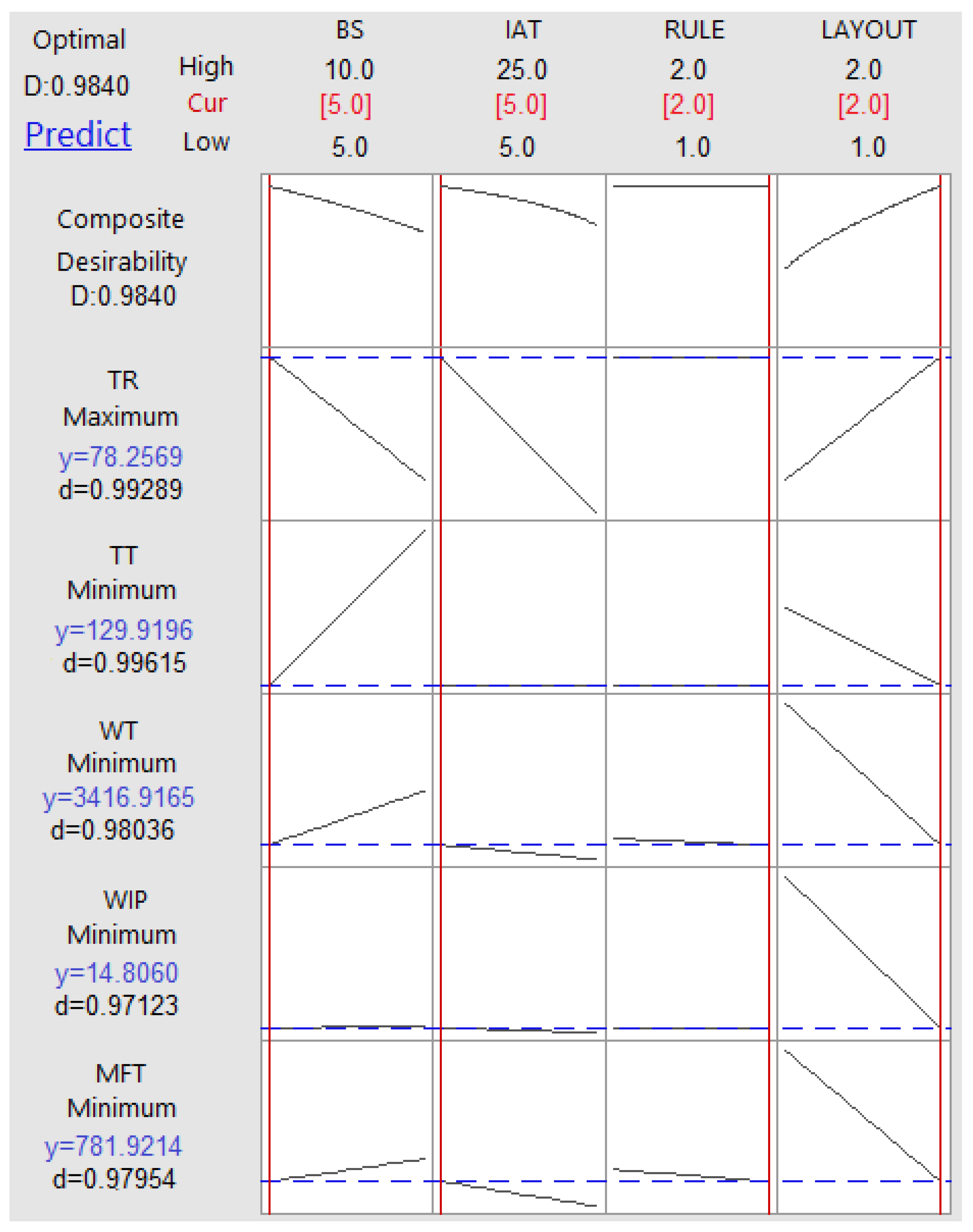
| DF | Optimized value | 781.921 | 14.806 | 78.257 | 129.971 | 3416.917 |
| Deviation value | +355.325 | +10.483 | −0.046 | +0.214 | +1769.234 | |
| Deviation in % | +83.293% | +242.494% | −0.059% | +0.165% | +107.377% | |
| GRA | Optimized value | 781.921 | 14.806 | 78.303 | 129.917 | 3416.917 |
| Deviation value | +355.325 | +10.484 | 0 | +0.160 | +1769.234 | |
| Deviation in % | +83.293% | +242.529% | 0% | +0.124% | +107.377% | |
| VIKOR | Optimized value | 428.164 | 4.409 | 14.195 | 129.757 | 1655.257 |
| Deviation value | +1.568 | +0.086 | −64.108 | 0 | +7.574 | |
| Deviation in % | +0.368% | +1.982% | −81.872% | 0% | +0.460% | |
| MOSO | Group | Optimization Result | Applicability | Rank |
|---|---|---|---|---|
| GP | A | + | − | 2 |
| DF | A | − | − | 4 |
| GRA | B | − | + | 3 |
| VIKOR | B | + | + | 1 |
Publisher’s Note: MDPI stays neutral with regard to jurisdictional claims in published maps and institutional affiliations. |
© 2022 by the authors. Licensee MDPI, Basel, Switzerland. This article is an open access article distributed under the terms and conditions of the Creative Commons Attribution (CC BY) license (https://creativecommons.org/licenses/by/4.0/).
Share and Cite
Jerbi, A.; Hachicha, W.; Aljuaid, A.M.; Masmoudi, N.K.; Masmoudi, F. Multi-Objective Design Optimization of Flexible Manufacturing Systems Using Design of Simulation Experiments: A Comparative Study. Machines 2022, 10, 247. https://doi.org/10.3390/machines10040247
Jerbi A, Hachicha W, Aljuaid AM, Masmoudi NK, Masmoudi F. Multi-Objective Design Optimization of Flexible Manufacturing Systems Using Design of Simulation Experiments: A Comparative Study. Machines. 2022; 10(4):247. https://doi.org/10.3390/machines10040247
Chicago/Turabian StyleJerbi, Abdessalem, Wafik Hachicha, Awad M. Aljuaid, Neila Khabou Masmoudi, and Faouzi Masmoudi. 2022. "Multi-Objective Design Optimization of Flexible Manufacturing Systems Using Design of Simulation Experiments: A Comparative Study" Machines 10, no. 4: 247. https://doi.org/10.3390/machines10040247