Article

Investigation of Hydrodynamic Performance and Evolution of the near Wake on a Horizontal Axis Tidal Turbine

1
Institute of Oceanographic Instrumentation, Qilu University of Technology (Shandong Academy of Sciences), Qingdao 266100, China
2
School of Ocean Technology Sciences, Qilu University of Technology (Shandong Academy of Sciences), Qingdao 266100, China
3
Sino-Ukrainian Ocean Acoustics Technology Innovation Center, Qingdao 266100, China
4
College of Mechanical and Electronic Engineering, Shandong University of Science & Technology, Qingdao 266590, China
5
College of Mechanical and Electronic Engineering, China University of Petroleum (East China), Qingdao 266580, China
*
Author to whom correspondence should be addressed.
Machines 2022, 10(4), 234; https://doi.org/10.3390/machines10040234
Submission received: 4 March 2022 / Revised: 24 March 2022 / Accepted: 24 March 2022 / Published: 27 March 2022
(This article belongs to the Section Turbomachinery)

Abstract

:
The hydrodynamic performance and near wake of tidal current turbines are investigated via numerical simulation and experimental methods in this study. Based on large eddy simulation, the performance and wake characteristics of a tidal 10 kW turbine are then studied at different TSR (Tip Speed Ratio), and the velocity deficit and wake expansion along the flow direction are compared. The equal proportion hydraulic turbine model is designed by the similarity theory, and the experiment was carried out in a water channel, the test parameters including power and torque. The simulation and experimental results show that due to the boundary effect and blocking effect of the flume, there is a certain deviation between the experimental data and the simulation data, but the trend is the same. With the increase of TSR, the pitch of the helix formed by tip vortex gradually decreases, and the tip vortex and root vortex are destroyed earlier in the process of moving downstream. The axial velocity deficit decreases with the increase of axial distance. Finally, the hydrodynamic performance of a turbine is analyzed through experiment and simulation. The experimental results verify and support the simulation results, but there are quantitative differences, and when the TSR = 5, the turbine efficiency has the maximum value.

1. Introduction

The marine energy power generation device mainly includes two parts: energy capture mechanism and conversion mechanism. The turbine blade responsible for energy capture is the core component of the whole power generation system, which is responsible for converting the kinetic energy of water flow into mechanical energy and then into electrical energy and other forms of energy. Although various forms of marine energy utilization have been developed, compared with other forms of power generation devices, horizontal axis and vertical axis turbines have the characteristics of high energy conversion efficiency and excellent starting performance, which has become a research hotspot all over the world [1,2,3].
At present, the widely used design theories of the horizontal axis tidal current turbine mainly include Betz theory, blade element momentum theory (BEM) and vortex theory. The mainstream design methods also include Glauert design method and Wilson method. In addition, the blade design methods include graphic method, simplified windmill design method, equal lift coefficient method, equal chord length method and optimization design method. According to the installation depth of the turbine, Noruzi et al. [4] designed the turbine by using the blade element momentum theory to improve the power coefficient. Neto et al. [5], using evolutionary algorithm to design wind turbine blades, reduces the number of cycles from aerodynamic to structural design in the traditional design process, so as to reduce the design time and cost. A 150-kW tidal turbine is designed by Goundar et al. based on BEM theory and the designed turbine has good efficiency under the water flow velocity of 1–3 m/s [6]. Tian et al. [7] designed a small-scale horizontal axis hydrokinetic turbine and evaluates the performance of the rotor both at transient and steady state. The design theory of tidal current turbine mostly comes from the wind turbine theory. The wind turbine design theory comes from various theories and methods of a propeller, such as lift line method [8] and vortex lattice method [9]. Considering the current development of turbine design, the main research focuses on the optimal design of a blade, which is based on the blade element theory and momentum theory, combined with the optimization method, and the relevant design software is launched. In addition to designing the turbine for hydrodynamic performance, considering the structural parameters, the design meets the requirements of strength and stiffness.
Many scholars have studied the wake vortex of hydraulic turbine, including the wake vortex model and vortex structure. Lam et al. [10] predicted the velocity distribution within a wake from a horizontal-axis tidal-current turbine using two novel analytical equations. Faizan et al. [11], using improved delayed detached eddy simulation, demonstrated that the model is capable of satisfactorily simulating the hydrodynamics of a horizontal axis tidal current turbine. Ebdon et al. [12] demonstrated that the turbulence intensity has a significant effect on the recovery of wake. In addition, the turbine operating condition also had an impact on the wakes. Lin et al. [13] focused on the vortex structure and energy conversion of hydraulic turbines and found that part of the flow kinetic energy has been converted into potential energy before reaching the rotor; commonly used power coefficients are not equivalent when quantifying energy extraction.
Gajardo et al. [14] analyzed flows with multiple turbines through experimental and numerical approaches and found that for downstream turbines, there is an accelerated wake development, increasing the temporal variability of the bed shear stress and the power and thrust coefficients. Modali et al. [15] used a combination of experimental and numerical simulation methods to characterize the performance and wake of tidal stream turbines. Vinod et al. [16] used an active-grid turbulence generator to mimic sheared-turbulent inflow representative of the flood (low shear) and ebb tides (high shear). The actuator surface model is used to simulate the tidal turbine, which reduces the number of grid elements and improves the accuracy of the wake [17]. Ma et al. [18] proposed two equations to predict the mean velocity within the wake of a vertical-axis turbine, and it is found that the formula can satisfactorily predict the wake vortex of a vertical axis turbine. In terms of turbine experimental methods, Zhang et al. [19] measured the effect of increasing ambient turbulence intensity on the wake of a three blade Tidal Turbine in a circulating water tank, and this is of great significance for studying the influence of wake propagation process. The downstream field of a single pile horizontal axis tidal turbine is experimentally studied by Zhang et al. [20]. Leroux et al. [21] used both quasi-steady and transient numerical approaches, and conducted a numerical study of the turbine wake, comparing it with the experimental results carried out by the French research team. In the region with low ambient turbulence level, wake velocity is closely related to turbulence recovery, and wake recovery is more significantly affected by lateral proximity [22]. The velocity loss behind the turbine is mainly caused by the kinetic energy extraction and the blocking effect of the rotor and support structure [23].
In this study, according to the blade element momentum theory, the numerical model of a 10 kW tidal current turbine is designed. In order to improve the computational accuracy, a large eddy simulation technique was employed. By analyzing the wake dynamic characteristics under different tip speed ratios, the variation law of vortex is found. Further, the variation law of turbine wake velocity loss and performance are measured by flume experiment, and the effect of these factors has also been carried out.

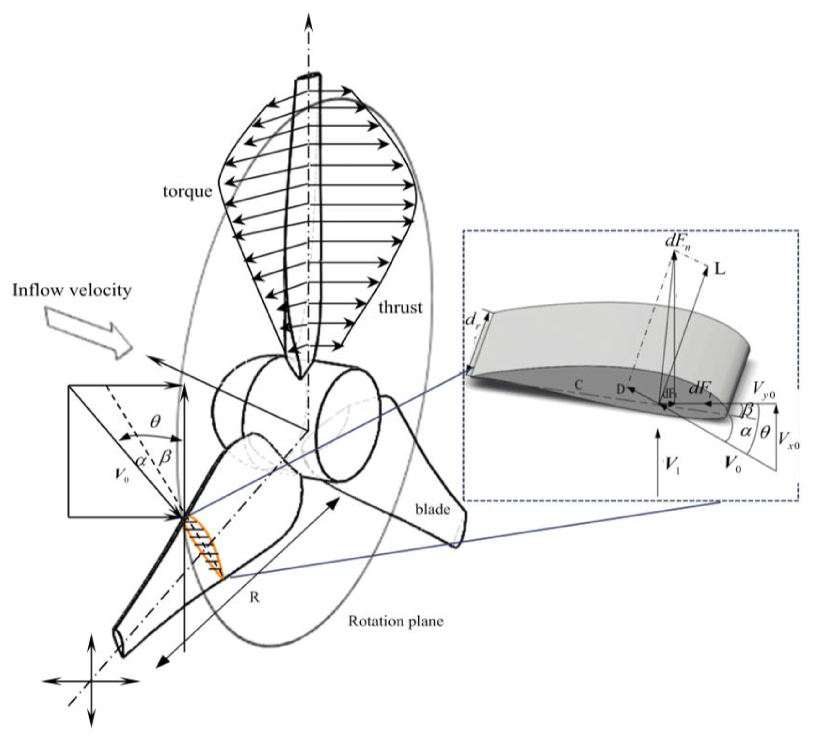
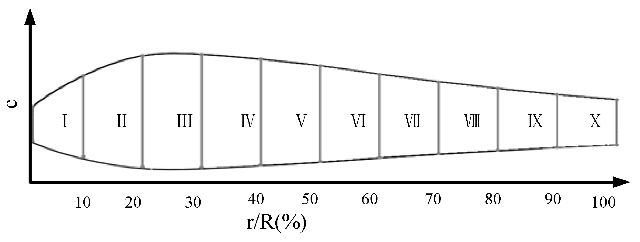
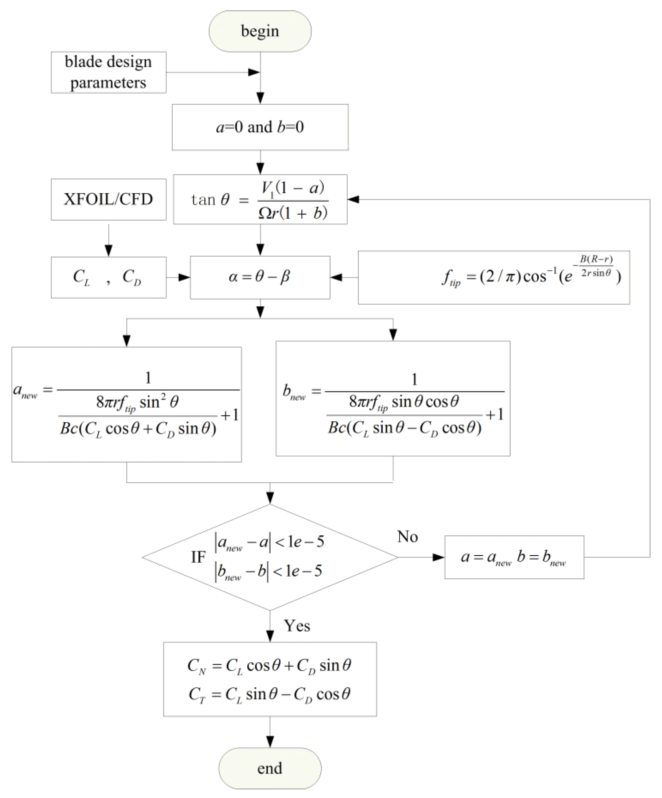
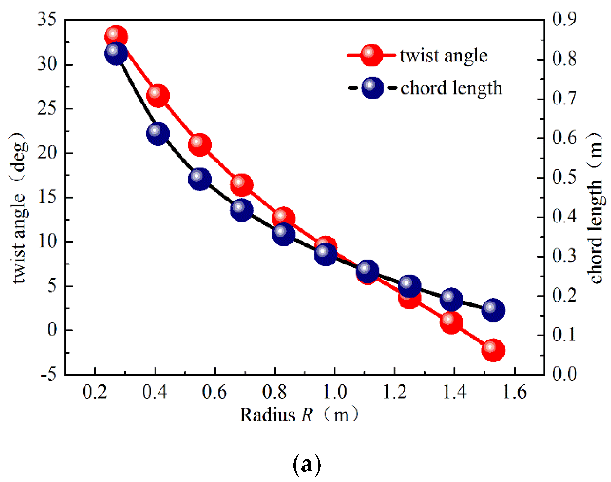
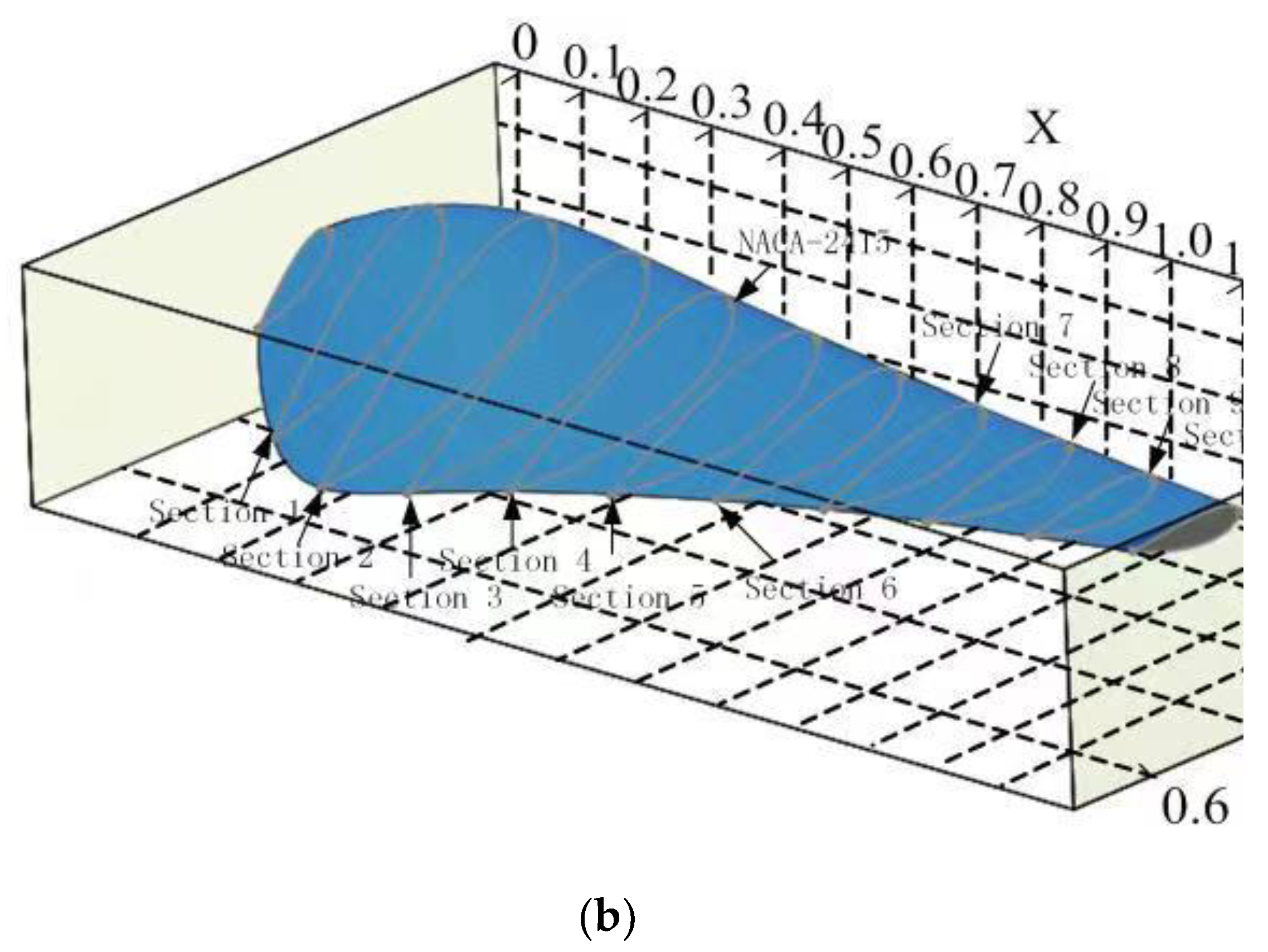
2. Turbine Blade Design

The Blade element theory was put forward by Richard Froude in 1889. Its basic idea is to divide the blade into several micro segments in the spanwise direction, and each segment is called a blade element, as shown in Figure 1. Assuming that there is no mutual interference between each blade element, the blade element is regarded as a two-dimensional airfoil, and the force it receives is only the lifting resistance of the airfoil. Then, the thrust and torque acting on the turbine can be calculated by summing the load acting on each blade element.
V 0 = V x 0 2 + V y 0 2 = ( 1 a ) 2 V 1 2 + ( 1 + b ) 2 ( Ω r ) 2
θ = α + β = arctan ( 1 a ) V 1 ( 1 + b ) Ω r
where V0 is the relative inflow velocity, V1 is the inflow velocity, Vx0, Vy0 are the velocity components of the inflow velocity (wind or water velocity) in the x and y directions respectively, Ω is the rotational angular velocity, α is the angle of attack, β is the twist angle, θ is the inflow angle, a, b is the axial induction factor and tangential induction factor, respectively.
Since the actual turbine is composed of a limited number of blades, Prandtl proposed a correction factor for blade tip loss, expressed as
f t i p = 2 π arccos ( exp ( B 2 R r r sin θ ) )
where B is number of blades, R is turbine radius and r is local radius.
The force acting on the blade element with length dr caused by relative inflow velocity V0 can be decomposed into normal force dFn and tangential force dFt
d F n = 1 2 ρ V 0 2 c C N d r
d F t = 1 2 ρ V 0 2 c C T d r
CN represents the normal force coefficient; CT represents the Tangential force coefficient; c represents the chord length.
C N = C L cos θ + C D sin θ
C T = C L sin θ C D cos θ
where CL is the lift coefficient and CD is the drag coefficient.
The lift on the blade element is expressed as
d L = 1 2 ρ V 0 2 c C L d r
d D = 1 2 ρ V 0 2 c C D d r
The blade with a length of R is divided into n (n = 10) segments, as shown in Figure 2 and the specific implementation steps are shown in Table 1:
According to the BEM calculation model written in MATLAB, combined with the momentum theoretical equation, the iterative cycle is carried out to solve the axial and tangential induction factors. The input includes the design parameters of blade, such as blade geometry, flow characteristics and aerodynamic coefficient, lift coefficient and drag coefficient of a blade section. The lift coefficient and drag coefficient is obtained by CFD, and the overall calculation code structure of BEM is shown in Figure 3.
The turbine that is numerically modeled in this study is the three-bladed turbine. The chord length and twist angle of the blade are shown in Figure 4a. At the same time, in order to better connect with the hub and control the overall size, the chord length at the blade root is corrected, and the final model is shown in Figure 4b.

3. Numerical Method

In this section, the CFD method is used to predict turbine performance and wake structure, and CFD method has been proved to be reliable and effective in many literature studies.

3.1. Large Eddy Simulation

Large eddy simulation (LES) is a turbulence numerical simulation method between direct numerical simulation (DNS) and Reynolds average method (RANS). The basic idea of large eddy simulation is to give up the instantaneous motion simulation of vortices in the full-scale range and only calculate the turbulent motion larger than the grid scale directly through the instantaneous Navier–Stokes equation. The Navier–Stokes equation is filtered to obtain the following equation [24,25,26]:
t ( ρ u ¯ i ) + x j ( ρ u ¯ i u ¯ j ) = p ¯ x i + x j ( μ u ¯ i x j ) τ i j x j
ρ t + x i ( ρ u ¯ i ) = 0
where ρ is the fluid density, p is the filtered pressure, ui is the filtered ith Cartesian velocity component.
The above formula constitutes the governing equations used in the large eddy simulation method.
τ i j = ρ u i u i ¯ ρ u ¯ i u ¯ j
τij is defined as sub grid scale stress, which reflects the influence of the motion of small-scale vortices on the solved motion equation.

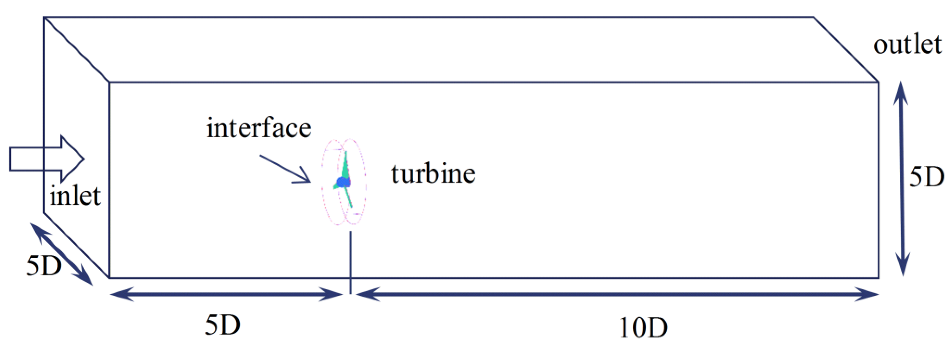
3.2. Computation Domains and Boundary Conditions

According to the rotation characteristics of the horizontal axis turbine, the calculation domain is set as shown in Figure 5. In order to facilitate grid division, the calculation domain is divided into internal turbine rotation domain and external stationary domain. The flow in the turbine rotation region is relatively intense, and the flow phenomenon on the blade surface needs to be observed. Therefore, the accuracy and quantity of the grid need to be improved. Due to the stable and uniform flow in the stationary region, grid accuracy is not required. In order to reduce the calculation time and cost, the number of grids here shall be reduced as much as possible. At the same time, in order to prevent the insufficient development of the flow field, the length of the calculation domain is 15 times the diameter of the internal rotation domain, and the length and width of the inlet is 5 times the diameter of the internal rotation domain.
The velocity inlet and pressure outlet are adopted, the inlet velocity is 0.5 m/s and the inlet turbulence intensity is set to 2%. Considering the transient action, the sliding grid will not cause the deformation and regeneration of the grid, nor form a negative volume. Through literature research, it has been found that the calculation results of the sliding grid can better present some typical hydrodynamic characteristics of the hydraulic turbine in practice [27], such as the spiral vortex caused by the blade tip, the steep slope velocity gradient around the blade and the adverse vibration load of the hydraulic turbine. Sliding grid technology is much more accurate in predicting turbine power and thrust, so it is used here. The rotation rate of the turbine is set by adjusting the velocity of the rotation domain. In this way, the simulation under different tip speed ratios can be realized.

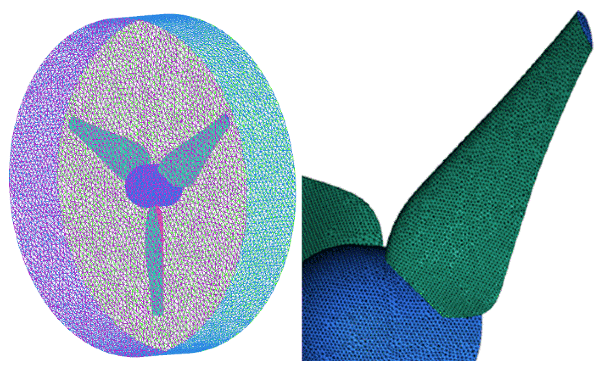
3.3. Grid Generation

In order to improve the calculation accuracy and reduce the calculation time, the grid division adopts the combination scheme of structured grid and unstructured grid; that is, the complex area of the internal turbine adopts unstructured grid, and the external static area adopts a structured grid. The specific grid quantity distribution is shown in Figure 6.
In order to study the influence of the change of grid density on the simulation results, the grid density in the blade area is changed by controlling the number of grids in the chord and spanwise directions of the blade, and the grid density in the calculation domain is changed by controlling the number of axial and radial grids in the calculation domain. Three groups of grids with different density are established and named Case I, Case II and Case III, respectively. Three grids are used to calculate the thrust coefficient of the turbine, and the results are shown in Table 2. It can be seen from the Table 2 that the calculation result of Case II is close to that of Case III, and the continuous increase of the number of grids has little impact on the calculation result. In order to save simulation time, Case II is selected for simulation calculation in this study.

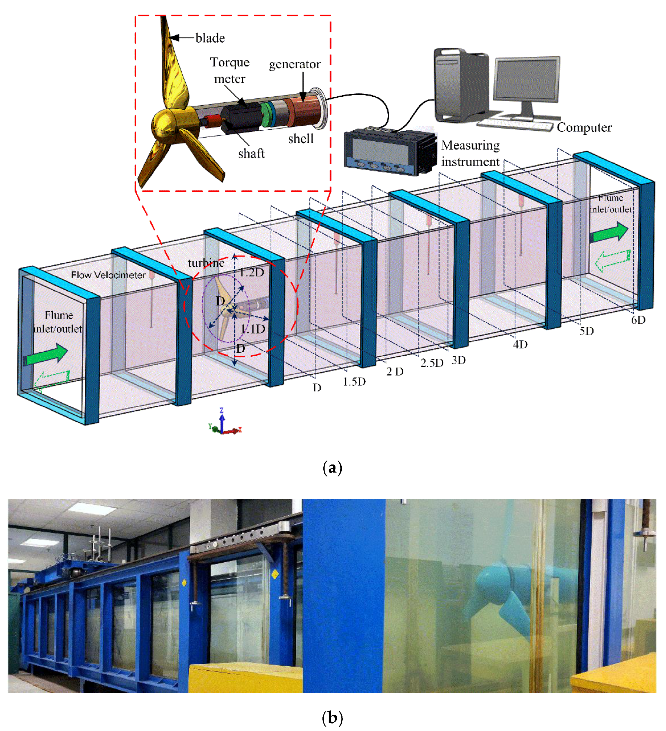
4. Experimental Arrangement

The test connection system of current (wave) making flume is shown in Figure 7. It is mainly composed of axial flow pump, open water tank, console and sensing and measuring instruments equipment. The high-power water pump makes the water circulate in a certain direction in the water tank to form a uniform and stable water flow to simulate the actual working conditions. An Acoustic Doppler Velocimeter was employed. In order to improve the accuracy, vertical points and longitudinal points were recorded, respectively. The accuracy of the probes is ±0.7%. The sample rate is 200 Hz, with a time length of 2 min. The specific structure, functions and parameters are as follows in Table 3.
For the designed turbine model, under the condition of fixed incoming flow velocity, adjust the load and change the torque to adjust the rotation rate and change the tip speed ratio. When there is no load, the variation curve of turbine velocity with incoming flow velocity is shown in Figure 8. Without any additional load, the turbine will rotate at a velocity that is mainly balanced by the rotating torque generated by blade lift and the resistance mainly from blade. The tip speed ratio is adjusted by changing the motor rotation rate and incoming flow velocity.

5. Results and Discussion

In order to observe the distribution of vorticity and velocity in the wake field of the turbine under different tip speed ratio, the influence of TSR on the turbine flow field is analyzed first. The downstream domain boundary was a constant pressure boundary with a gauge pressure of 0 Pa, and the incoming flow speed is set as 2 m/s. As shown in Figure 9 when TSR = 2, a relatively stable spiral shedding vortex is formed at the blade tip, with clear vortex trace and large pitch. In the process of downstream development, the vortex gradually collapses, and spiral shedding vortex is also formed at the hub. The hub vortex is concentric with the blade tip vortex, but the diameter is small. The pitch of the hub vortex is significantly larger than the blade tip vortex, but the velocity is lower than the blade tip vortex. Similarly, in the process of propagating downstream, the vortex will gradually dissipate, and its intensity will gradually decrease. With the increase of TSR, the pitch of spiral vortices formed at the tip decreases gradually. As shown in Figure 10, when TSR = 4, the pitch of spiral vortices generated at the tip decreases significantly compared with that when TSR = 2. This is due to the increase of turbine rotation rate, the increase of the number of spiral vortices generated at the same time and the decrease of axial moving velocity of tip shedding vortices. Due to the small pitch of adjacent shedding vortices, the interference between them is almost mixed together to form a closed cylindrical surface, which also collapses rapidly at the downstream. Figure 11 shows the turbulence intensity and velocity distribution of turbine and wake flow field. Due to the blocking effect of a turbine, a relatively long low-speed zone is formed in the front and rear of blade tip and hub, especially in the rear. With the increase of TSR, the diameter of the low-speed zone also increases, but the axial length decreases, and the intensity and range of the low-speed zone formed at the blade tip also increase with the increase of the blade tip speed ratio; the speed boundary behind the turbine is also more obvious. When the tip velocity is relatively small, a horn-shaped strong turbulent basin is formed behind the hub, and an annular strong turbulent zone is formed at the tip. The turbulence intensity increases with the increase of tip speed ratio.
Keeping the incoming flow velocity unchanged and adjusting the tip speed ratio by changing the turbine rotation rate, the incoming flow speed is set as U0 = 0.6 m/s. The speed at the point of the rear section of the turbine is defined as U. The transverse velocity distribution curves of numerical results from 0.5D to 6D downstream result from 1.5D to 5D and are given in Figure 12. As shown in Figure 12, the lateral velocity distribution downstream at x = 1.5D, x = 3D, and x = 5D indicates the wake development of a horizontal axis tidal turbine. Obviously, due to the blocking effect of the hub, the velocity deficit behind the hub is the largest, forming an obvious valley bottom.
When the TSR = 1, at x/D = 1.5, x/D = 3, x/D = 5, the numerical and experimental results fit well, as shown in Figure 13; however, from the experimental results, the velocity deficit value is less than the numerical simulation value. At the bottom of the valley, the experimental value is 6.49% higher than the simulated value, while at the same time, the experimental results show that the transverse velocity of the wake recovers faster due to the boundary effect of flume. Because the flow around the turbine is limited by the side wall of the water tank, the stress of the turbine caused by the increase of the flow velocity is different from the real sea state. The size boundary of numerical simulation is much larger than that of the experiment; the influence of boundary effect is small.
When the TSR = 2, the velocity deficit value at each section becomes larger compared with TSR = 1 from the numerical simulation results. Similarly, at x/D = 1.5, x/D = 3, x/D = 5, the experimental results show that the bottom value also decreases. This is due to the increase of turbine rotation rate and resulted in an increased turbine blocking effect, which, in turn, increased the downstream velocity deficit.
When the TSR = 3, due to the increase of rotating velocity, the blocking effect of the turbine is further strengthened. All in all, although there are some differences between the two groups of data, the experimental results have the same trend as the numerical simulation results. The first reason for the difference is the blocking effect of the turbine itself, and the size of the experimental tank is limited, which leads to the obvious influence of boundary effect.
By adjusting the incoming flow velocity and load, change the turbine rotation rate, adjust the TSR, and verify the turbine power coefficient and torque parameters. As shown in Figure 13, each group of tests adopts three different rotation rates: 78 rpm, 104 rpm and 122 rpm, respectively. Therefore, the Reynolds number is different at different velocity of the same TSR. Due to the dimensional constraints of the test equipment, the variation range of Reynolds number is small. The Reynolds number can be calculated according to the incoming flow velocity and the size of the tank. The variation range of Reynolds number is about Re = 1.6 × 10⁵~5.6 × 10⁵, affected by incoming flow velocity and turbine rotation rate. For three different velocity conditions, the Reynolds number has an obvious impact on the power coefficient and torque coefficient. Generally, the higher the Reynolds number, the higher the efficiency when the tip speed ratio is high. When the TSR is less than 5, the power coefficient decreases with the increase of velocity. When it exceeds 5, the turbine has a high-power coefficient under high velocity conditions. The expression of power coefficient CP is
C P = 8 λ 2 R 4 0 R b ( 1 a ) r 3 d r
where λ = ΩR/V1 a and b is the axial induction factor and tangential induction factor, respectively.
The red and blue curves represent the power coefficients at two different turbine rotation rates, and the power coefficient is affected by the following factors.
f ( a , b ) = b ( 1 a )
The inflow velocity is different in the two cases, and the axial inducers and tangential inducers may also be different. In fact, when the tip speed ratio is less than 6, the turbine power coefficient at low rotation rate is higher than the other two. There is a certain difference between the two, but the value is small.
Figure 14 and Figure 15 are the variation curves of turbine torque and torque coefficient with blade tip speed ratio. When the tip speed ratio is less than 4.5, the turbine torque coefficient at a low rotation rate is higher. However, when the tip speed ratio is greater than 5, the opposite is true. When the turbine speed is high, it has a large torque coefficient. At the same incoming velocity, the torque coefficient CQ increases first and then decreases with the increase of tip speed ratio. For torque, with the increase of tip speed ratio, the torque Q decreases without changing the velocity. Under the same tip speed ratio, the higher the incoming velocity, the greater the output torque.

6. Conclusions

In this paper, the turbine model is established for numerical simulation and experimental research, and the large eddy simulation method is used to analyze the dynamic characteristics of turbine wake. At the same time, the law of turbine wake velocity loss is verified by experiments, and the following conclusions are obtained:
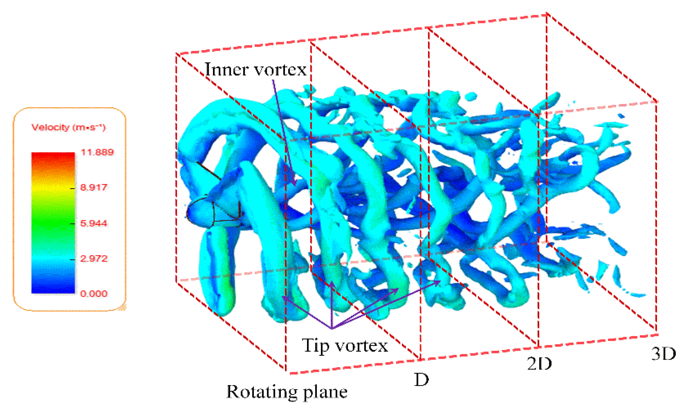
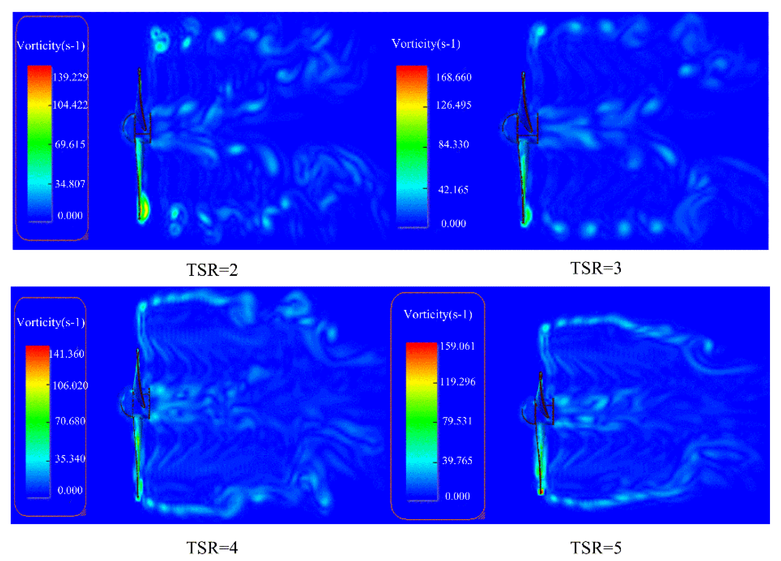
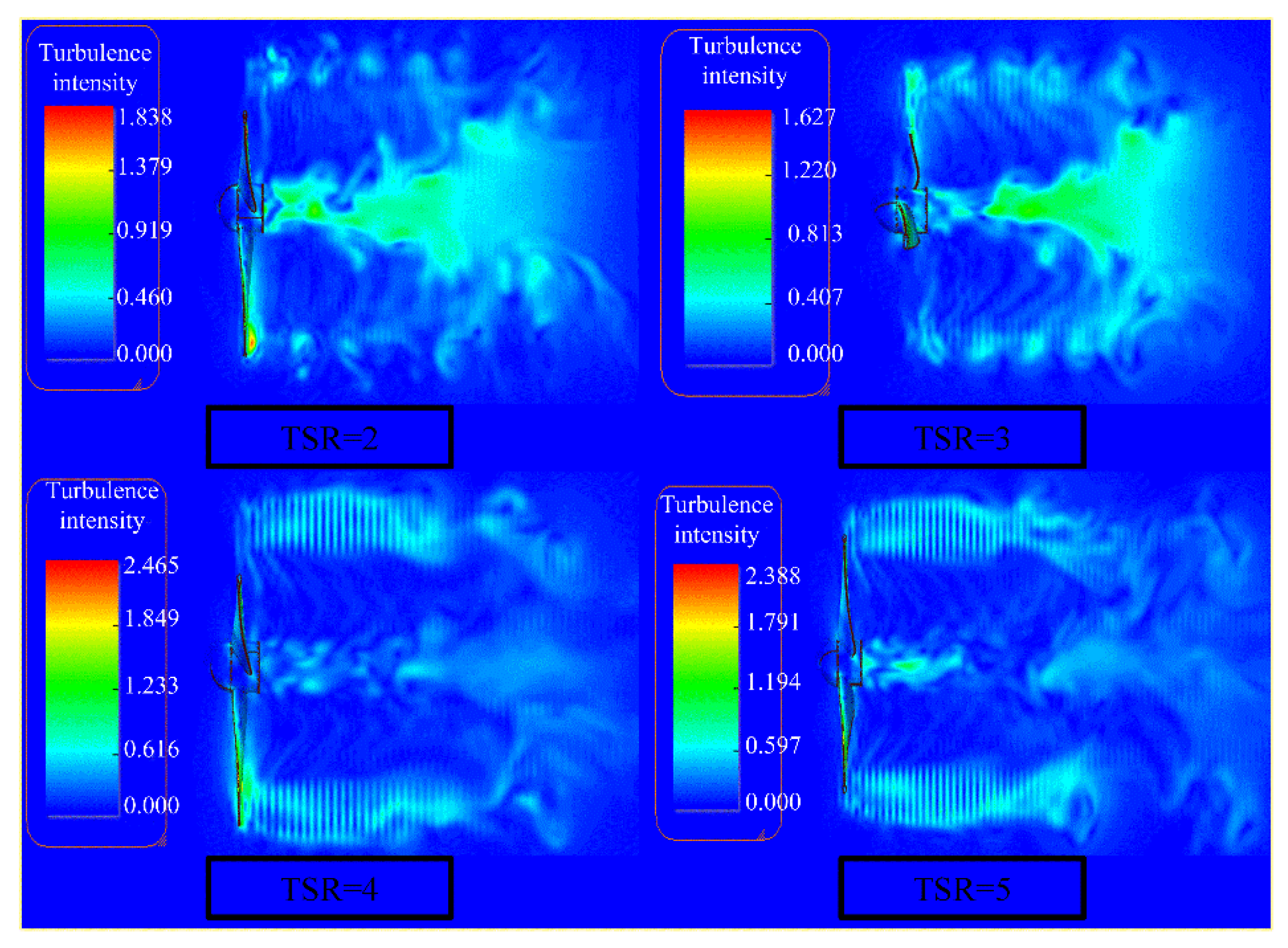
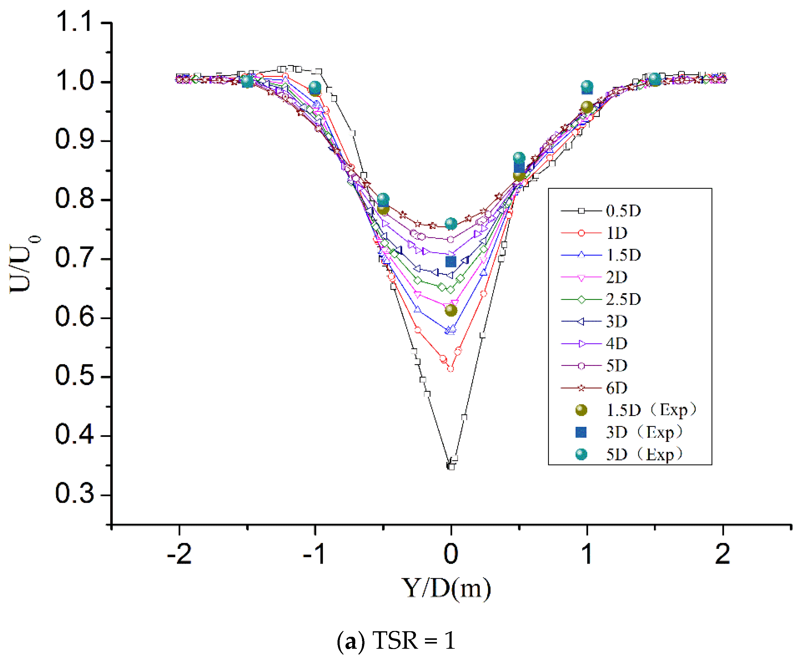
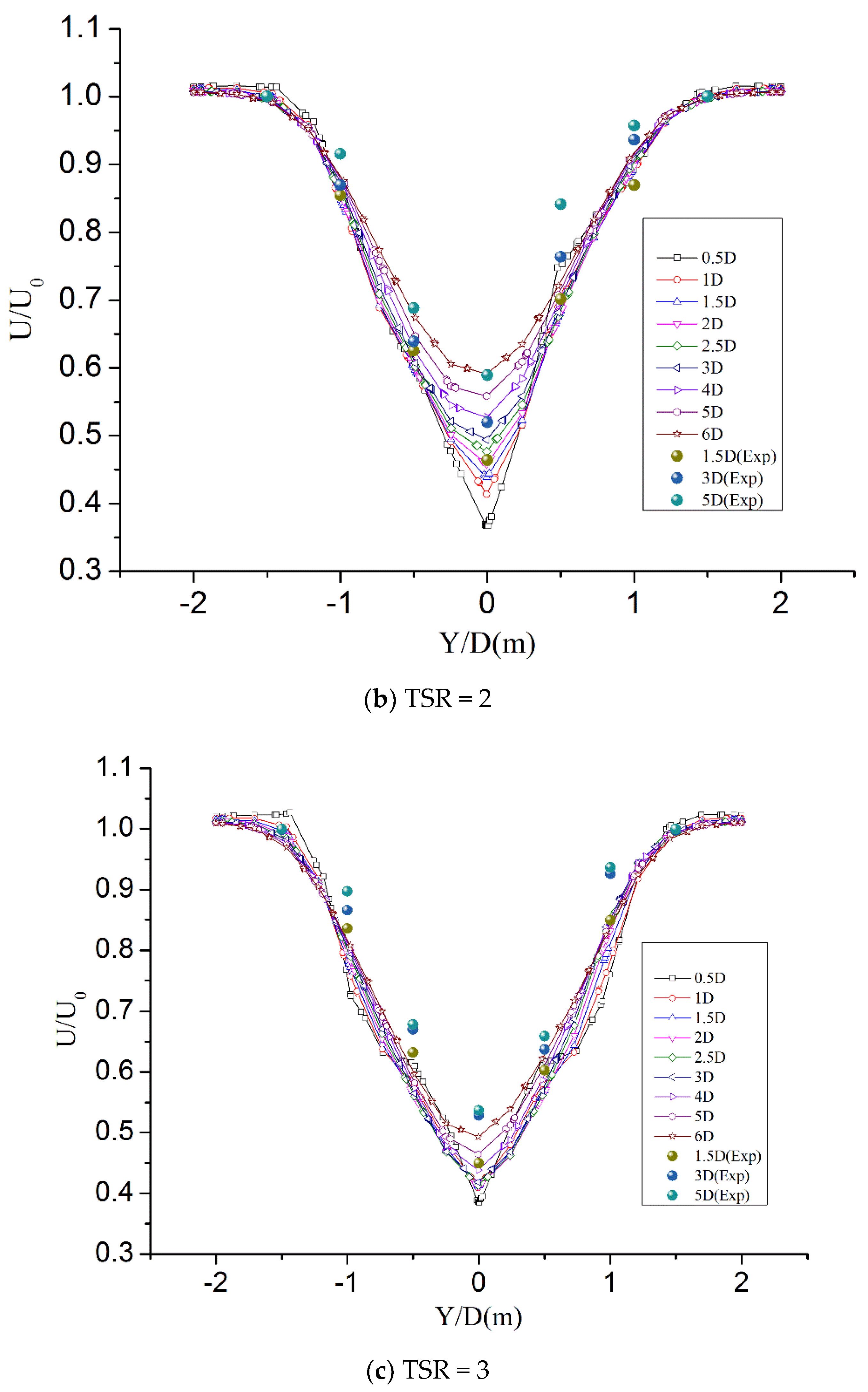
  • The numerical simulation and experimental results show that at the downstream position of the turbine, the velocity deficit curve changes with the position, and the velocity deficit at the downstream position of the hub shows a decreasing trend. The velocity deficit also shows a decreasing trend with the direction of blade spanwise. With the increase of TSR, the pitch of the helix formed by tip vortex decreases gradually, and the vortex generated at the root and tip of the blade collapses earlier.
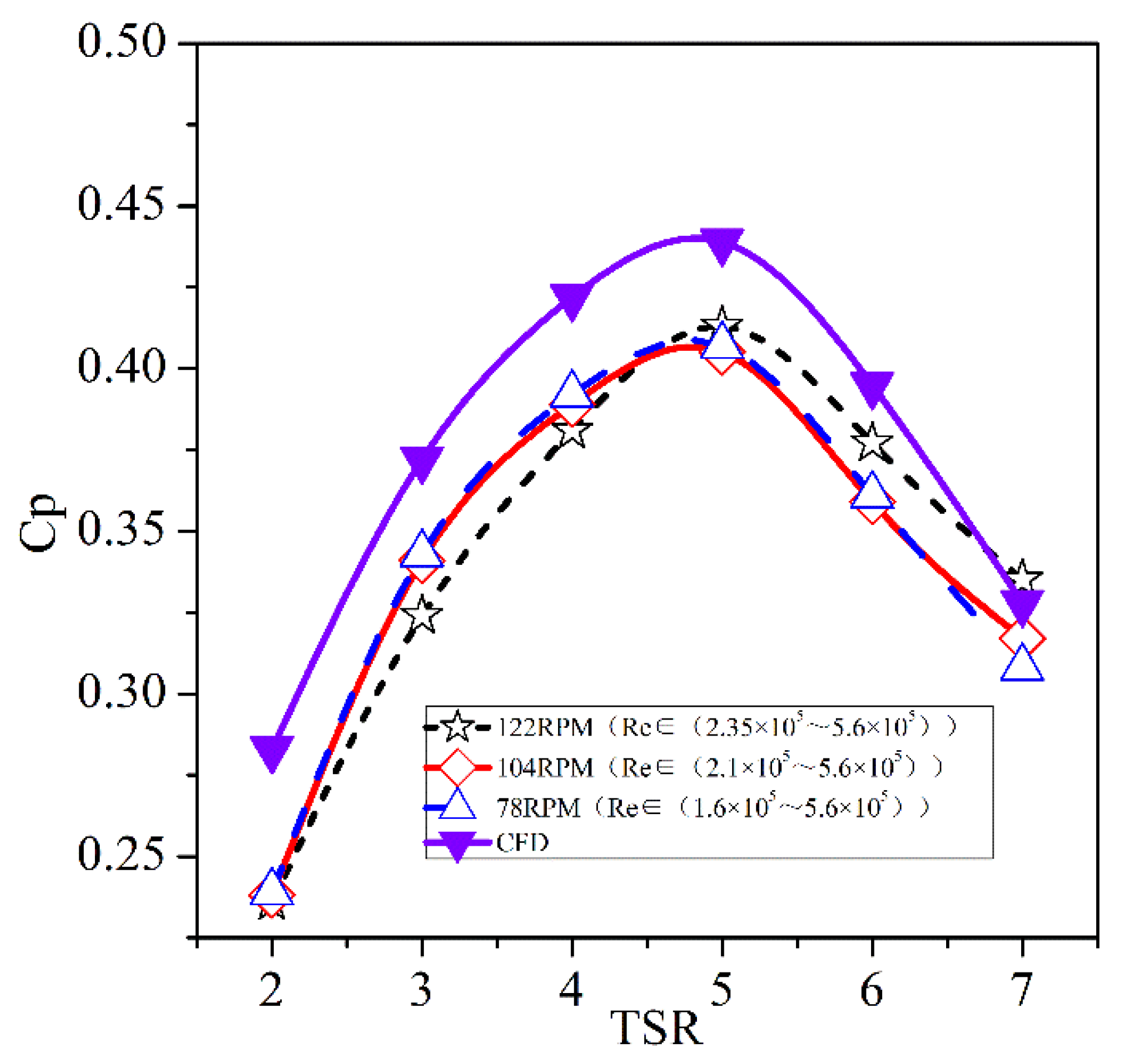
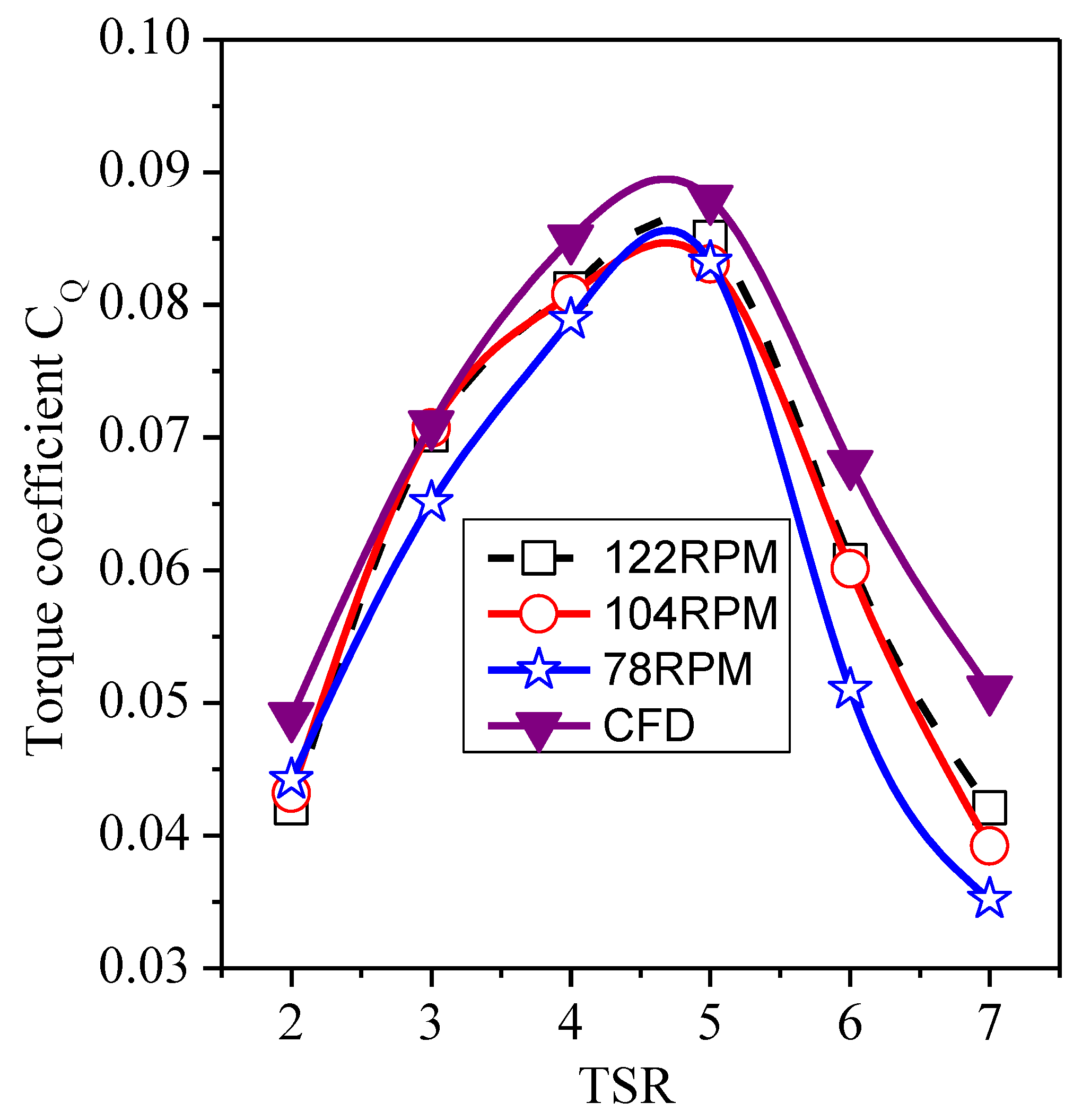
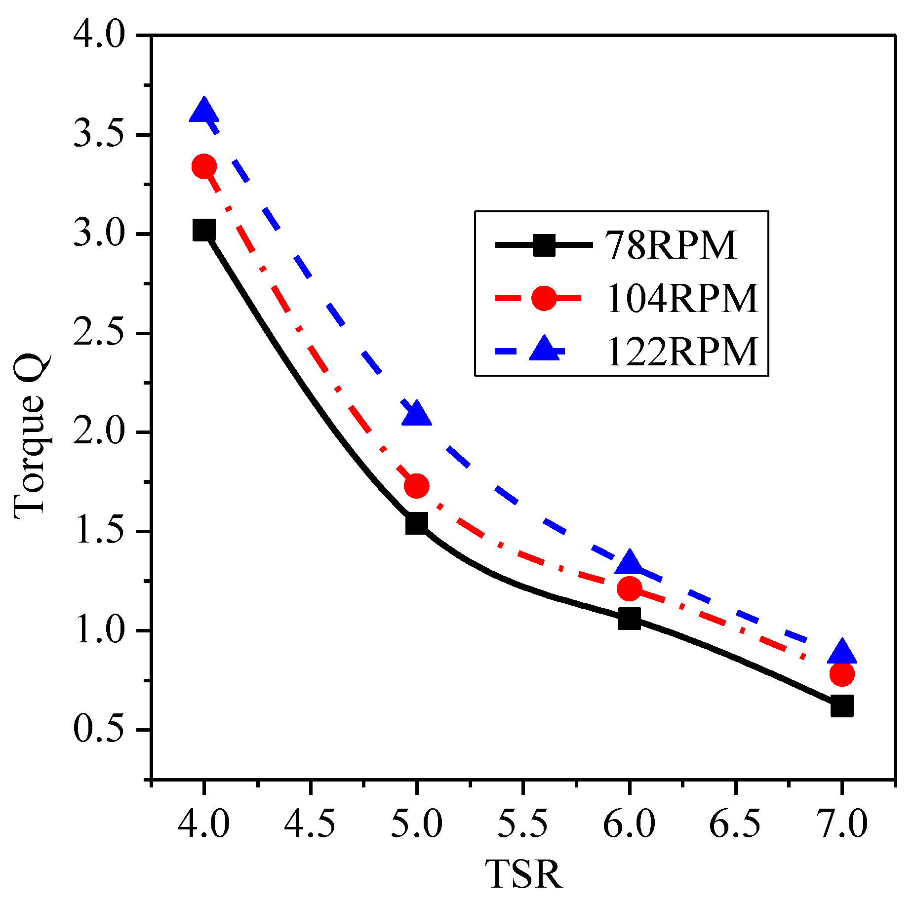
  • There is an optimal tip speed ratio range for turbine operation. The parameters such as turbine power and torque predicted by the experimental values are different from those predicted by the numerical simulation, but the trend fits well. Because the water flow around the turbine is limited by the side wall of the water tank, the speed of the water flow is forcibly increased, resulting in the difference between the stress condition of the turbine and the simulation condition. When the tip speed ratio is about 5, the designed turbine power coefficient reaches the maximum.
  • In addition, through the comparison between experiment and numerical simulation, it is proved that large eddy simulation (LES) has certain accuracy and advantages in predicting wake vortex trace.

Author Contributions

Conceptualization, Z.S.; Formal analysis, L.F.; Funding acquisition, Y.M.; Methodology, Y.Z. and M.F.; Resources, D.L.; Software, C.G. and C.L. All authors have read and agreed to the published version of the manuscript.

Funding

This research was funded by the Natural Science Foundation of Shandong Province (Program No. ZR2020QA045).

Institutional Review Board Statement

Not applicable.

Informed Consent Statement

Not applicable.

Data Availability Statement

Not applicable.

Conflicts of Interest

The authors declare no conflict of interest.

Nomenclature

aAxial induction factor
bTangential induction factor
BNumber of blades
cChord length
CLLift coefficient
CDDrag coefficient
CTThrust coefficient
CNTorque coefficient
fPrandtl’s tip loss factor
CPPower coefficient
V1Inflow velocity
V0Relative inflow velocity
ReReynolds number
αAngle of attack
βTwist angle
θInflow angle
ρLiquid density
ΩAngular velocity of the rotor
rLocal radius
RRadius of whole turbine
pthe filtered pressure
uithe filtered ith Cartesian velocity component
τijsubgrid scale stress
TSRtip speed ratio

References

  1. Alamian, R.; Shafaghat, R.; Amiri, H.A.; Shadloo, M.S. Experimental assessment of a 100 W prototype horizontal axis tidal turbine by towing tank tests. Renew. Energy 2020, 155, 172–180. [Google Scholar] [CrossRef]
  2. Elie, B.; Oger, G.; Guillerm, P.-E.; Alessandrini, B. Simulation of horizontal axis tidal turbine wakes using a Weakly-Compressible Cartesian Hydrodynamic solver with local mesh refinement. Renew. Energy 2017, 108, 336–354. [Google Scholar] [CrossRef]
  3. Su, H.; Dou, B.; Qu, T.; Zeng, P.; Lei, L. Experimental investigation of a novel vertical axis wind turbine with pitching and self-starting function. Energy Convers. Manag. 2020, 217, 1–14. [Google Scholar] [CrossRef]
  4. Noruzi, R.; Vahidzadeh, M.; Riasi, A. Design, analysis and predicting hydrokinetic performance of a horizontal marine current axial turbine by consideration of turbine installation depth. Ocean. Eng. 2015, 108, 789–798. [Google Scholar] [CrossRef]
  5. Neto, J.X.V.; Junior, E.J.G.; Moreno, S.R.; Ayala, H.V.H.; Mariani, V.C.; Coelho, L.d.S. Wind turbine blade geometry design based on multi-objective optimization using metaheuristics. Energy 2018, 162, 645–658. [Google Scholar] [CrossRef]
  6. Goundar, J.N.; Ahmed, M.R. Design of a horizontal axis tidal current turbine. Appl. Energy 2013, 111, 161–174. [Google Scholar] [CrossRef]
  7. Tian, W.; Mao, Z.; Ding, H. Design, test and numerical simulation of a low-speed horizontal axis hydrokinetic turbine. Int. J. Nav. Archit. Ocean Eng. 2018, 10, 782–793. [Google Scholar] [CrossRef]
  8. Melo, D.B.; Baltazar, J.; de Campos, J.A.C.F. A numerical wake alignment method for horizontal axis wind turbines with the lifting line theory. J. Wind Eng. Ind. Aerodyn. 2018, 174, 382–390. [Google Scholar] [CrossRef]
  9. UsAr, D.; Bal, Ş. Cavitation simulation on horizontal axis marine current turbines. Renew. Energy 2015, 80, 15–25. [Google Scholar] [CrossRef]
  10. Lam, W.H.; Chen, L. Equations used to predict the velocity distribution within a wake from a horizontal-axis tidal-current turbine. Ocean Eng. 2014, 79, 35–42. [Google Scholar] [CrossRef]
  11. Faizan, M.; Badshah, S.; Badshah, M.; AliHaider, B. Performance and wake analysis of horizontal axis tidal current turbineusing Improved Delayed Detached Eddy Simulation. Renew. Energy 2022, 184, 740–752. [Google Scholar] [CrossRef]
  12. Ebdon, T.; Allmark, M.J.; O’Doherty, D.M.; Mason-Jones, A.; O’Doherty, T.; Germain, G.; Gaurier, B. The impact of turbulence and turbine operating condition on the wakes of tidal turbines. Renew. Energy 2021, 165, 96–116. [Google Scholar] [CrossRef]
  13. Lin, J.; Lin, B.; Sun, J.; Chen, Y. Wake structure and mechanical energy transformation induced by a horizontal axis tidal stream turbine. Renew. Energy 2021, 171, 1344–1356. [Google Scholar] [CrossRef]
  14. Gajardo, D.; Escauriaza, C.; Ingram, D.M. Capturing the development and interactions of wakes in tidal turbine arrays using a coupled BEM-DES model. Ocean. Eng. 2019, 181, 71–88. [Google Scholar] [CrossRef] [Green Version]
  15. Modali, P.K.; Vinod, A.; Banerjee, A. Towards a better understanding of yawed turbine wake for efficient wake steering in tidal arrays. Renew. Energy 2021, 177, 482–494. [Google Scholar] [CrossRef]
  16. Vinod, A.; Han, C.; Banerjee, A. Tidal turbine performance and near-wake characteristics in a sheared turbulent inflow. Renew. Energy 2021, 175, 840–852. [Google Scholar] [CrossRef]
  17. Bai, G.; Li, G.; Ye, Y.; Gao, T. Numerical analysis of the hydrodynamic performance and wake field of a horizontal axis tidal current turbine using an actuator surface model. Ocean. Eng. 2015, 94, 1–9. [Google Scholar] [CrossRef]
  18. Ma, Y.; Lam, W.H.; Cui, Y.; Zhang, T.; Jiang, J.; Sun, C.; Guo, J.; Wang, S.; Lam, S.S.; Hamill, G. Theoretical vertical-axis tidal-current-turbine wake model using axial momentum theory with CFD corrections. Appl. Ocean. Res. 2018, 79, 113–122. [Google Scholar] [CrossRef] [Green Version]
  19. Zhang, Z.; Zhang, Y.; Zhang, J.; Zheng, Y.; Zang, W.; Lin, X.; Fernandez-Rodriguez, E. Experimental study of the wake homogeneity evolution behind a horizontal axis tidal stream turbine. Appl. Ocean Res. 2021, 111, 102644. [Google Scholar] [CrossRef]
  20. Zhang, Y.; Zhang, J.; Lin, X.; Wang, R.; Zhang, C.; Zhao, J. Experimental investigation into downstream field of a horizontal axis tidal stream turbine supported by a mono pile. Appl. Ocean Res. 2020, 101, 102257. [Google Scholar] [CrossRef]
  21. Leroux, T.; Osbourne, N.; Groulx, D. Numerical study into horizontal tidal turbine wake velocity deficit: Quasi-steady state and transient approaches. Ocean Eng. 2019, 181, 240–251. [Google Scholar] [CrossRef]
  22. Nuernberg, M.; Tao, L. Experimental study of wake characteristics in tidal turbine arrays. Renew. Energy 2018, 127, 168–181. [Google Scholar] [CrossRef] [Green Version]
  23. Chen, Y.; Lin, B.; Lin, J.; Wang, S. Experimental study of wake structure behind a horizontal axis tidal stream turbine. Appl. Energy 2017, 196, 82–96. [Google Scholar] [CrossRef]
  24. Ahmadi, M.H.B.; Yang, Z. The evolution of turbulence characteristics in the wake of a horizontal axis tidal stream turbine. Renew. Energy 2020, 151, 1008–1015. [Google Scholar] [CrossRef]
  25. Ahmadi, M.B. Influence of upstream turbulence on the wake characteristics of a tidal stream turbine. Renew. Energy 2018, 132, 989–997. [Google Scholar] [CrossRef] [Green Version]
  26. Menon, S.; Yeung, P.K.; Kim, W.W. Effect of sub-grid models on the computed inter-scale energy transfer in isotropic turbulence. Comput. Fluid 1996, 25, 165e180. [Google Scholar] [CrossRef]
  27. Mcnaughton, J.; Afgan, I.; Apsley, D.D.; Rolfo, S.; Stallard, T.; Stansby, P.K. A simple sliding-mesh interface procedure and its application to the CFD simulation of a tidal-stream turbine. Int. J. Numer. Methods Fluids 2014, 74, 250–269. [Google Scholar] [CrossRef]
Figure 1. Velocity triangle and force analysis of blade element section.
Machines 10 00234 g001
Figure 2. Span locations for blade.
Machines 10 00234 g002
Figure 3. Flow chart of the code structure of the BEM.
Machines 10 00234 g003
Figure 4. (a) Distribution of chord length and twist angle of blade (b) Three-dimensional model.
Machines 10 00234 g004aMachines 10 00234 g004b
Figure 5. Schematic view of the computational domain.
Machines 10 00234 g005
Figure 6. Grid model.
Machines 10 00234 g006
Figure 7. (a) Water channel (b) Experimental prototype.
Machines 10 00234 g007
Figure 8. The relationship between the rotation and the velocity of incoming flow.
Machines 10 00234 g008
Figure 9. Instantaneous view of vortex structures in the flow field.
Machines 10 00234 g009
Figure 10. Vortex distribution of plane in different TSR.
Machines 10 00234 g010
Figure 11. Turbulence intensity distributions in different TSR.
Machines 10 00234 g011
Figure 12. (a) The velocity profile downstream in TSR = 1 by CFD and experiment. (b) The velocity profile downstream in TSR = 2 by CFD and experiment. (c) The velocity profile downstream in TSR = 3 by CFD and experiment.
Machines 10 00234 g012aMachines 10 00234 g012b
Figure 13. The variation of power coefficient with TSR at different sets of RPMs.
Machines 10 00234 g013
Figure 14. Torque coefficient CQ changes with TSR.
Machines 10 00234 g014
Figure 15. Torque Q changes with TSR.
Machines 10 00234 g015
Table 1. Classical BEM.
Classical BEM
Input date: radial position and turbine radius, angular velocity of the rotor, velocity in ambient free stream, number ofblades (r, Ω, V0, B)
Divide the blade into 10 sections, and set initial values for a and b (axial and tangential induction factors);
Calculate the inflow angle tan θ = V 1 ( 1 a ) Ω r ( 1 + b ) ,   α = θ β .  
Calculate lift and drag coefficients (CL & CD) according to CFD or experimental data.
Calculate the tip loss factorftip (Prandtl).
Calculate anew and bnew.
Calculate CT, CN
Table 2. Comparison of calculation results.
TypeMesh NodesIteration StepsCT
Case I3.43 × 1065000.514
Case II3.84 × 1065000.552
Case III4.36 × 1065000.557
Table 3. Equipment parameters.
ProjectParameterMemos
Sink size parameter (length, width and height)16,000 (mm) × 800 (mm) × 1400 (mm)
Maximum water depth1000 mm
Turbine diameter600 mm
Dynamic torque sensor measuring range0–20 NmThe error range is 0.1%
Incoming flow velocity range0.00~1.50 (m/s)The error range is 1.5%
TSR range1–6
Publisher’s Note: MDPI stays neutral with regard to jurisdictional claims in published maps and institutional affiliations.

