Article

Modeling Impulsive Ball Mill Forces Effects on the Dynamic Behavior of a Single-Stage Gearbox

by
Gauthier Ngandu Kalala
1,2,
Xavier Chiementin
1,
Lanto Rasolofondraibe
3,*,
Abir Boujelben
1 and
Bovic Kilundu
4
1
Institute of Thermics, Mechanics and Material (ITheMM), University of Reims Champagne-Ardenne, Moulin de la Housse, 51687 Reims, France
2
Polytechnic Faculty, University of Lubumbashi, Kasapa, Lubumbashi 7110502, Congo
3
Centre de Recherche en STIC (CReSTIC), University of Reims Champagne-Ardenne, Moulin de la Housse, 51687 Reims, France
4
Mechanical Section, Higher Institute of Applied Technology (ISTA), Kinshasa 1021101, Congo
*
Author to whom correspondence should be addressed.
Machines 2022, 10(4), 226; https://doi.org/10.3390/machines10040226
Submission received: 1 March 2022 / Revised: 17 March 2022 / Accepted: 19 March 2022 / Published: 23 March 2022
(This article belongs to the Section Machines Testing and Maintenance)

Abstract

:
Gearboxes are frequently used in the mining industry, especially for power transmission between the electric drive and the ball mill; besides the extreme complexity of a ball mill gear transmission system, the fault diagnosis by vibration analysis can be easily distorted by the presence of impulsive noises due to the ball pulses on the mill shell. Although several works in the literature are related to the influence of an impulsive noise on the accuracy of the diagnosis, no dynamic model exists yet in the literature that can explain the influence of these forces on the dynamic behavior of gearboxes. This paper presents a new approach to determine the influence of the grinding forces in crack defects diagnosis. This approach is based on a hybrid numerical model of a 24-degree-of-freedom gearbox, simulating one gear train and two drive shafts. The impact forces of the mill drum are modelled by a discrete element method (DEM). The ball-filling rate ( F r ), the mill speed ( N r ), and the ball size ( D b ) are considered to study this phenomenon. The simulations results show by a time series representation, fast Fourier transform, and short-time Fourier transform (STFT), that the acceleration is significantly affected by the presence of the grinding forces, developing an impulsive noise due to the impact of the balls governed by the studied parameters.

1. Introduction

Ore treatment process is an essential step in the mining industry. The goal is to reduce it to a desired particle size by using a ball mill, to be then treated chemically or physically [1]. This process is most often associated with high operating costs. About 70% of these costs are attributed to the particle reduction range from 30–50 mm to 20–50 micron [2,3]. Research should be carried out to reduce these costs by exploring different solutions, for example, (i) optimizing the energy consumed by the ball mills [4,5], (ii) automation of the grinding process [6,7,8], or (iii) optimization of maintenance operations. The main purpose of industrial maintenance is to ensure the availability of the production tools. If well applied, it can also contribute efficiently to a reduction of the operating costs of the machines. Industrial maintenance has undergone a continuous evolution over the years, advancing from a corrective to a preventive approach. However, the drawback of this approach is the risk to intervene too late when a failure has already occurred before the next scheduled maintenance, or replacing parts too early, which might have been still functional before failure. However, this could be corrected by a so-called conditional preventive approach according to which an intervention is decided based on the measured state of the equipment.
Vibration analysis has long been the main tool for monitoring rotating machines and is therefore highly represented in the industry. It operates based on the properties of impulsivity and periodicity of disturbances related to a localized fault. However, when applied to nonstationary operating conditions and impulsive environments such as in the mining industry, it shows a lack of precision to detect mechanical defects. The monitoring methods using vibration analysis developed in the context of rotating machines should be accurate in order to ensure a reliable diagnosis. To obtain satisfactory results, real conditions in which the monitored equipment operates must be considered. Through modeling and simulation, it is becoming increasingly possible to understand certain complex phenomena normally rather difficult to obtain directly in an industrial environment. This paper focuses on the vibration behavior of gearboxes driving ball mills in the mining industry, which often operate in a harsh environment due to shocks and collisions on the mill drum.
Research has already focused on these issues, particularly in the context of gear modeling. The first trend focuses on the consideration of varying operating conditions. This research seeks to understand, with the help of modeling, the consequences that fluctuations in loading and/or speed can have on the diagnosis of gear defects by vibration analysis. F. Chaari et al. [9] proposed a model for the variation of the gearing stiffness based on the mechanical characteristics of the drive motor and the loading conditions. Simulation results on a single-stage spur gear transmission led to frequency modulations in perfect agreement with experimental results. W. Bartemus and R. Zimroz [10] demonstrated through a concentrated mass modeling and an experimental investigation the sensitivity of a gear transmission in terms of vibration level and increasing loading conditions. They showed that a defective transmission is more sensitive to increased load by generating higher vibrations. N. Baydar and A. Ball [11] concluded that a spectral analysis cannot track the degradation of a gear’s condition under fluctuating load conditions. They used the instantaneous power spectrum to detect local defects in the teeth of a gear under different load conditions. Farhat et al. [12] developed a numerical model of single-stage gears subjected to variable speed and load conditions and studied their influences in the presence of combined gear and bearing faults.
Other researchers have been interested in the environment, in which most rotating machines operate, mainly in the mining industry. The presence of shocks, impulses, and collisions of materials that characterize most mining processes is often highlighted. It has been observed that the vibration signatures collected in these processes are most often contaminated by the presence of noncyclic impulsive shocks at high energy. This phenomenon makes it difficult to extract useful information about the monitored machine faults. Stochastic signal modeling approaches are most often used for these types of processes. G. Yu and N. Shi [13], for example, proposed a new method of statistical modeling of gear defects based on an α-stable distribution. A. Wylomanska et al. [14] also proposed a method for separating the useful signal related to the bearing fault from a noncyclic and non-Gaussian impulsive noise, in the context of monitoring a raw material crusher. The proposed technique was applied to a simulated signal as well as a real signal. S. Schmidt et al. [15] suggested the synchronous median of the square of the envelope method, instead of the synchronous mean of the square of the envelope of a vibration signal, for fault diagnosis of gearboxes operating under variable conditions and in an impulsive environment. This study showed its effectiveness on simulated and real signals. Jacek w et al. [16] proposed to use nonnegative matrix factorization of spectrogram for separation cyclic and noncyclic impulsive components from a hammer crusher. Jacek w. [17] proposed the time-varying spectral kurtosis (TVSK) as a means of spectral kurtosis adaptation for frequency-band selection of bearing damage signals under variable operating conditions. In a corresponding trend, Hebda-Sobkowicz et al. [18] presented a new approach to local bearing damage detection in the presence of non-Gaussian impulsive noise based on conditional variance statistics to identify cyclic and noncyclic impulses. This method allows to detect and extract cyclic-impulsive signal (damage in bearing) in the presence of high amplitude noncyclic impulsive signal. Several other researchers have addressed the issue in this sense [19,20,21].
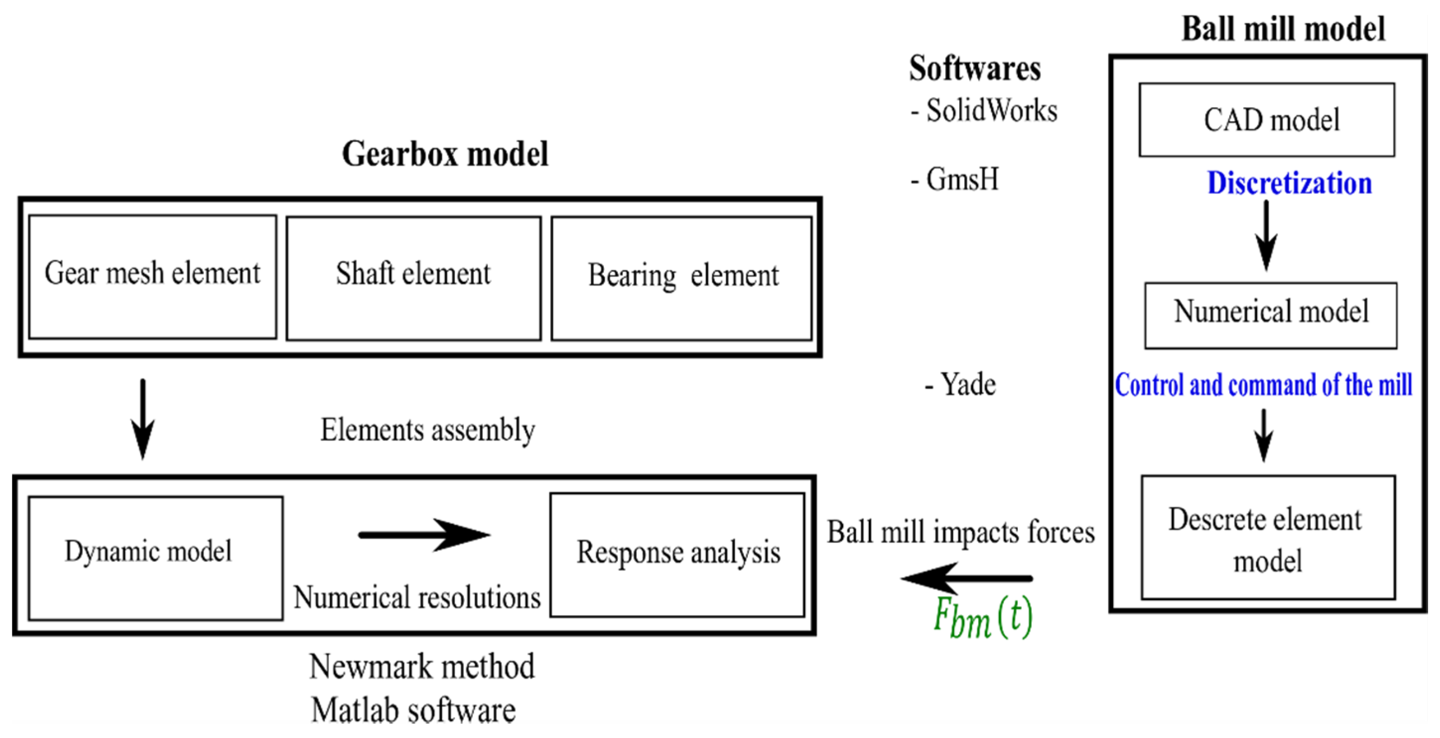
Gearboxes driving ball mills in the mining industry are subject to impulsive forces created by the falling of the balls and ore against the mill drum. The vibratory characteristics of the gears leading to a fault detection can be affected by the presence of these forces/shocks, which makes it difficult to detect localized faults in the gearboxes. However, in the literature, no numerical model allows us so far to understand the vibratory behavior of gearboxes in an impulsive environment such as that generated by the ball mill. The lack of knowledge of the nature of the forces generated by the fall of the balls against the mill drum does not permit us to develop an efficient mathematical model that characterizes the distribution of these forces. For modeling gears in an impulsive environment, the common practice is to synthesize the signal, considering it as a combination of several components: a deterministic component which often characterizes the manifestation of the fault, a gaussian random component which models noise, and a non-Gaussian random component which models impulsive noise. The weakness of this method is that the modeled signal can only describe one type of defect at a time. In this paper, a new hybrid numerical approach is proposed, combining two types of models: (i) a classical model of a gear transmission (lumped parameter model and finite elements models for gear and shaft), (ii) a discrete element model of a ball mill. The second model simulates the internal behavior of the ball mill and provides the grinding forces that will be considered as external efforts in the model of the transmission. The objective is to show, using this model, the influence of impulsive grinding forces on the transmission vibratory behavior in the presence of defects. In addition to the introduction and the conclusion, the paper is organized into three main sections. Section 2 presents the general methodology of the hybrid approach giving details on the software and the design of the simulation to be performed. Section 3 focuses on the description of the gearbox model and the ball mill model separately. 
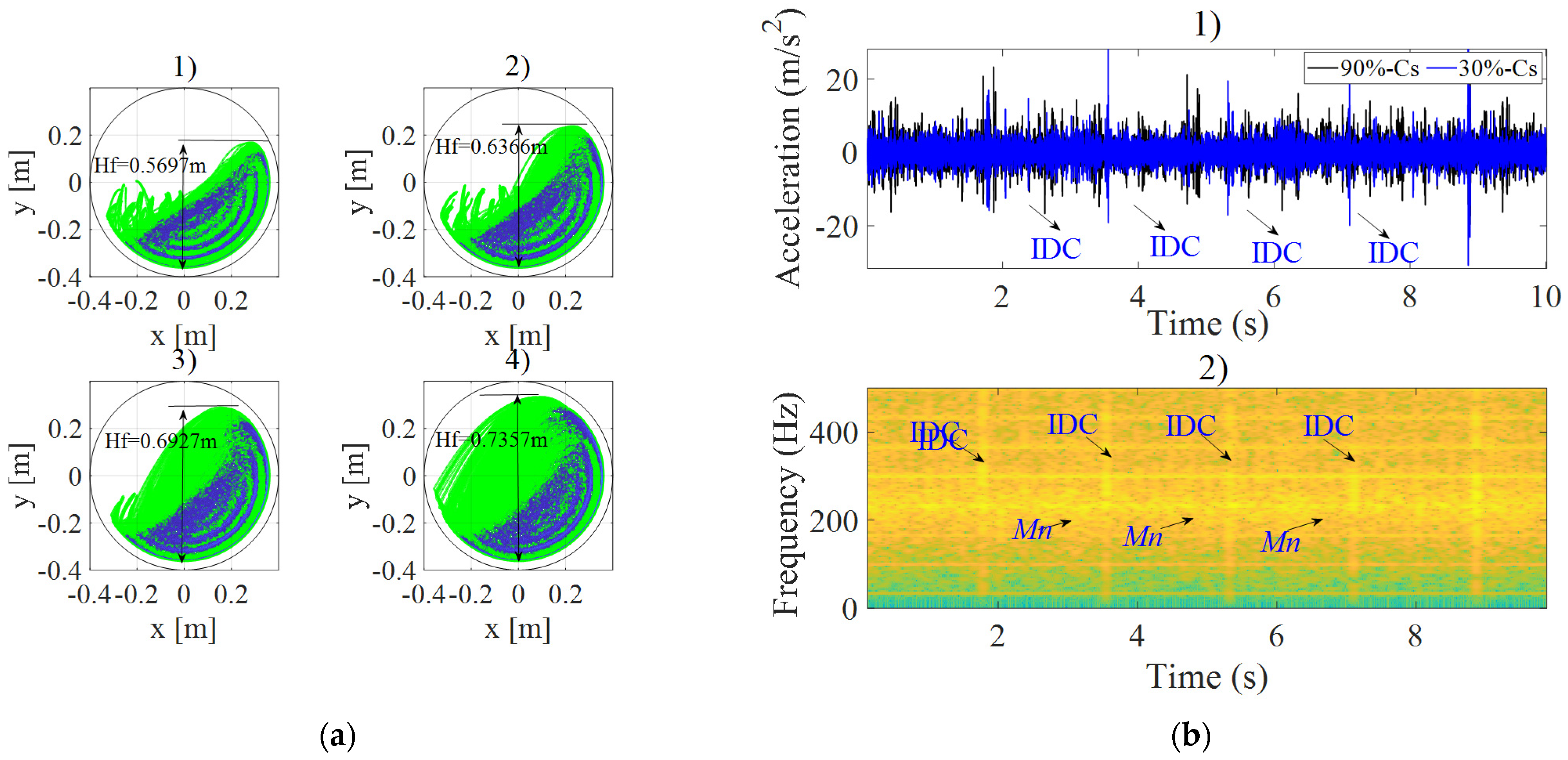
Section 4 presents results; first, the load profile and the shape of the grinding forces are presented, then the influences of its forces are studied in healthy and under crack fault conditions, respectively.

2. Methods

2.1. Introduction

In industrial reality, a ball mill is generally made of a cylindrical drum driven by an electric motor via a gear reducer. In addition to the gear reducer, a ring gear is directly connected to the mill, whose transmission is provided by an external pinion, thus yielding an additional reduction stage. The model studied in this paper is a simplified version in accordance with a laboratory setup in which the mill is mounted at the end of the gearbox output shaft (Figure 1). During its rotation, the mill drum lifts the charge along one side until it reaches the maximum drop height. From this position, the particles start to fall independently of the drum movement, described by either a cascade or a cataract movement depending on the rotation speed of the mill [3].
By falling against the drum, particles’ impact forces are created and transmitted to the gearbox through the drive shaft. Despite the presence of a lining to absorb the impacts, the impact forces produced by the movement of the load inside the mill are present and their amplitude can increase with the wear of the lining. It is therefore necessary to study their influence on the dynamic behavior of the gearbox.

2.2. Methodology

The methodology implemented in this work is presented in the (Figure 2). It is based on a modeling approach called hybrid, which consists of bringing together different types of models for each technological element involved in the system. Three technological elements were involved in this model. The drive shafts were modeled by a finite element method, using Timoshenko beam elements. Gears were described by a lumped parameter model and were located on their corresponding nodes on the two input and output shafts; the ball mill was represented by a discrete element method. The geometry of their shell, produced by computer-aided design software such as SolidWorks and/or FreeCAD, can be loaded from many commonly used formats such as a mesh produced by Gmsh software [22]. The discretized model was loaded using a Python program; spherical particles were filled in a ball mill and run using discrete elements modeling in Yade software. By solving Newton’s second law, the trajectory of every particle was calculated, so the properties and behavior of the material under the influence of different external forces may be observed. By observing the trajectory and postprocessing of the collected data either in Yade or an external program such as ParaView, a deeper understanding of the microscopic processes may be obtained [23]. After obtaining impulsive forces and assembling each element, the calculated forces were applied to the 24-degree-of-freedom gearbox model and were solved using the Newmark time integration scheme in (MATLAB), to study the dynamic response.

2.3. Simulation Design

During the operation of the mill, the rotational speed, filling rate, and ball size are operating parameters that can change during the process and influence in different ways the dynamics of the load inside the mill, and consequently, of the entire structure [4]. The mill speed is defined as the percentage of the critical speed   C s . The critical speed C s of the mill is the rotation speed at which the balls are subject to centrifugal force while adhering to the inner surface of the drum [4,24,25]. It can be calculated by the following Equation (1).
C s = 42.3 D M
where D M   is the average diameter of the mill. The critical speed of the mill simulated in this paper was 5.04 (rad/s). Four speed levels from 30% to 95% of this speed were considered. The filling rate F r is the fraction of the internal volume of the mill occupied by the circulating load. The four simulated filling rates ranged from 5% to 35% and the simulated mill was successively fed with balls of diameter ranging from 30 to 120 mm. The choice of these three parameters is justified by the fact that their influence has been noticed through industrial observations during the grinding process. For example, the reduction in ball size due to wear leads to an outward ejection of the balls. This phenomenon has a direct influence on the filling rate. It is often decided to increase the number of balls to achieve the filling rate required for grinding ores. Moreover, the rotation speed of the mill affects the type of ore grain size and varying this speed can often adjust the grain size at the outlet of the mill by. The grinding can therefore be carried out in cascade or cataract modes, depending on whether the rotation speed is close to or far below the critical speed. Table 1 shows how the simulations were designed according to the three operating parameters.

3. System Modeling

3.1. Modeling of the Gearbox

  • The transmission system studied in this work was a single-stage gearbox, according to the bench SURVIB of the laboratory of mechanical engineering of the URCA. It consists of two transmission shafts, two gears, four bearings, and a housing. Some assumptions were made in the modeling of the gears:
  • The influence of the housing was neglected.
  • The shafts were assumed to have constant cross sections.
  • The wheel and the pinion were rigid, the only deformation being at the contact point, and the connection was flexible, with a variable mesh stiffness.
  • The contact between wheel and pinion was assumed to be frictionless.

3.1.1. Gear Element

The chosen gear model considered the work previously carried out by [26] in the context of wind turbine gearboxes. In his work, the developed model allowed us to connect the node N 1 of the wheel to the node N 2 of the pinion as described in (Figure 3b), by linking through a stiffness matrix K g e a r     the restoring forces transmitted to the displacements X g e a r , (Figure 3a), as expressed by Equations (2) and (3).
{ F g e a r } = [ K g e a r ] { X g e a r }
and
[ K g e a r ] = k m [ G ]
The stiffness matrix [ K e n g ]   of the gear element can be expressed as a product of a matrix [G] including the elements describing the geometry of the gear (radii of the base circles, pressure angle α, and an average mesh stiffness k m , which can be estimated according to ISO 6336 [27]). The matrix [G] is calculated by considering that the strain energy associated with this average stiffness is equal to:
E p = 1 2 k m ·   Σ 2 = 1 2 k m ( { σ } T · { X g e a r } ) 2 = 1 2 k m ( { X g e a r } [ G ] { X g e a r } T )
[ G ] = σ T σ
where σ is the geometric vector of the gear transmission and defined by Equation (6):
σ = { c 0 c λ 1 μ 1 s + d 1 c λ 1 c c 0 s λ 2 s d 2 c μ 2 s λ 2 c }
{ X g e a r } is the generalized gear displacement vector defined by:
{ X g e a r } = [ x p   y p   θ p   x g   y g   θ g ] gear
The parameters involved in Equation (6) are described in Table 2 for a two-mesh configuration depending on the type of loading.
R p and R g are, respectively, the radii of the pinion and wheelbase circle; α and β, are, respectively, the pressure angle and the helix angle of the tooth in contact.
The modeling led to the determination of the mesh rigidity matrix as described in Appendix A. Compared to the work of [26] in which the meshing stiffness was assigned a constant, a variable meshing stiffness was considered in this work, in order to describe the manifestations of meshing defects. However, nonlinear bearing forces were not dealt with in this case. Due to the variation of the number of teeth in contact during meshing, the duration of the contact depends on the contact ratio ε and the variation of the meshing stiffness can be modeled by a square function (Figure 4) K g e a r   ( t ) , according to the work done by [9,12]. It fluctuates around a mean value k m   and can be described by Equation (8)
K g e a r ( t ) = { K 2               0 t ( ε 1 ) T m K 1               ( ε 1 ) T m t T m
where T m   is the meshing period, ε is a contact ratio, and K 1   and K 2     are the minimum and maximum values corresponding to the contact stiffness when one or two teeth are in meshing. A crack defect can be introduced to the model, by cyclically weakening the mesh stiffness by a degradation rate calculated by Equation (9):
D ( t ) = α δ [ 1 + n sin ( n α π ) n α π cos ( n Ω i t ) ]
In the presence of this defect, the meshing rigidity is thus calculated by:
K ( t ) = K ( t ) [ 1 D ( t ) ]
with 0 < D(t) < 1, and Ω i = 2π f i , f i , representing the rotation frequency of the wheel affected by a crack. δ and α = 1⁄ Z i are the amplitude of the function D(t), and the cyclic ratio, respectively. Table 3 gives the different parameters used for the gear simulation.

3.1.2. Shaft Element

The shaft of the gearbox was assumed to be flexible in bending and torsion and made of a homogeneous material, to have a constant cross section, and to have small displacement in bending. An energetic approach based on the Lagrange formalism was applied. The two shafts were discretized into 6 elements including 8 nodes, as shown in (Figure 5) to approximate the displacement field. Unlike the work carried out by [28], the 3-degree-of-freedom in Equation (11), corresponding to one rotation along the z-axis and two translations along x and y were retained in each node to describe the system. The nodal displacement vector {χ} is defined in Equation (12):
{ χ } n o d e = { x ,   y ,   θ } node
The vector containing the displacement fields over an element is given by:
{ χ e } = { x 1 , y 1 , θ z 1 , x 2 , y 2 , θ z 2   }
Thus, the model has a total of 24 degrees of freedom (Figure 5). The adequate choice of shape functions and application of Lagrange’s equations led to the determination of elementary mass M e and rigidity K e matrixes of the shaft element, as described in Appendix B. The motor and the load were accounted for by their respective masses and polar inertias. They were concentrated at node 1 of the input shaft and node 8 of the output shaft, respectively. The bearings, modeled by constant rigidities mounted in parallel, supported the shafts. The geometric and material properties of the shafts are reported in Table 4.

3.2. Discrete Element Modeling of the Ball Mill

3.2.1. Principle

The discrete element method is used to simulate the motion and interactions of discrete particles in a dynamic environment such as a ball mill. This method uses contact models for an accurate characterization of the contact forces between the particles during their motion. In this paper, a process based on the discrete element method was developed and implemented in Yade in order to determine the motion of the charge and to calculate the interaction forces between the ball and the mill drum. The numerical model of the mill had therefore two main components: first, a geometric component that represents the geometry of the surface with which the balls come into contact (Figure 6a); second, a contact model that describes the interactions between the modeled particles and a drum as well between the different particles (Figure 6b). Three different elements were considered in the simulation: spherical elements representing the balls, triangulated surfaces representing shell liner and planes representing end walls.
Considering a set of particles whose motion is described by Newton’s second law, the linear contact model shown in Figure 6b models the forces acting on each particle. In ball mills modeling, these particles are usually spheres representing the balls. The following properties characterized each sphere j: (i) properties of states such as the position of the center x bj , the linear speed bj , the angular speed   ω   bj , the linear acceleration x ¨ bj , the angular acceleration ω ˙ bj , the forces applied to their centers F bj , and the moment of force, i.e., the torque about the center M bj ; (ii) shape properties such as diameter d bj or the radius   r bj of each particle; (iii) material properties such as density ρ bj and contact parameters. These spheres move in space according to Newton’s second law (in translation and rotation) as follows:
{ m bj x ¨ bj = F bj I bj ω ˙ bj = M bj
where m bj = 4 π ρ bj r bj 3 3 ,   I bi = 2 m bj r bj 2 5 ,   are, respectively, the mass and the moment of inertia, and F bj represents the mechanical contact forces. For elastic particles, F bj was determined using the classical contact theory.

3.2.2. Model of Contact between Particles

The interactions between the balls and the mill wall can be dealt with by means of a suitable contact law. Both gravity and friction effects were considered. A linear contact law was used to determine the normal contact forces F n , and tangential forces F s [29];
The normal force F n was calculated based on the relative displacement   δ n , created during the interaction between the sphere and the contact surface. It was expressed as follows:
F n =   K n δ n + η n d δ n dt
where K n   and   η n are, respectively, the stiffness and the viscosity coefficients in the normal direction. The tangential force F s was defined by the following relation:
F s = min ( μ F n ,   K s v s dt + η s v s )
It consists of the frictional force   μ F n , where μ is the friction coefficient acting between the particles, and the force due to the spring and the damping in the shear direction exceeding μ F n . η s   represents the viscosity coefficient in the tangential direction and v s is the velocity in the same direction. Table 5 gives different parameters used in the ball mill simulation.
The equations of motion described by Equation (13) were solved numerically, using an explicit integration scheme called the “Leapfrog” algorithm implemented in Yade software, and described by the following equation.
{ q ˙ ( t + δ t 2 ) = q ˙ ( t δ t 2 ) + q ¨ ( t ) δ t   q ( t + δ t ) = q ( t ) + q ˙ ( t + δ t 2 )
where q ,   δ t ,   and   t , are, respectively, the generalized position vector of the sphere mass centers, the constant time step, and the current time. This algorithm is conditionally stable. To ensure the stability of the algorithm, the time step should be less than the critical time step δ t cr given by:
δ t cr = 2 ω max
ω max being the highest frequency in the system [30].

3.3. Equations of Motion

The above-described elements were assembled to obtain the finite element model. The latter was governed by a 24-equation system corresponding to the 24 degrees of freedom described in Section 3.1.2. Equation (18) represents the described model as a matrix equation.
[ M ] { X ¨ } + [ C ] { X ˙ } + [ K ] { X } = { F B M ( t ) } + { F ext ( t ) }
where F e x t ( t )   is the vector of external forces applied to the gearbox, consisting of the motor torque   C M ( t ) , and the resistive torque of the mill C R ( t ) . F B M ( t )   represents the vector of forces exerted by the mill.
F B M ( t ) = [ zeros ( 1 , 21 ) F BMx ( t ) F BMy ( t ) zeros ( 1 , 1 ) ]
and
F e x t ( t ) = [ zeros ( 1 , 2 ) C M ( t ) zeros ( 1 , 18 ) C R ( t ) ]    
The vectors F B M x ( t ) and F B M y ( t ) are point vectors corresponding to the values of the forces exerted by the balls on the mill drum and calculated separately using Yade software. [ M ] ( 24 × 24 ) and [ K ]   ( 24 × 24 ) are, respectively, the mass matrix and the stiffness matrix of the gearbox, obtained by assembling the elementary matrices of the system components. { X } ( 24 × 1 ) is the vector of degrees of freedom of the global system. [ C ]   ( 24 × 24 ) represents the global damping matrix, calculated proportionally to the mass matrix   [ M ] ( 24 × 24 ) and the average value of the stiffness matrix [ K ]   ( 24 × 24 ) as follows:
C = α [ M ] + β [ K ]
α   and   β are two real coefficients calculated so that the damping is viscous. According to [31], all resolution schemes for which α = 1 / 2 and β = 1 / 4 are unconditionally stable. In this work, the resolution of the system of equations was conducted using the standard Newmark integration scheme. The mill torque (resistive torque)   C R , the driving torque C M , and the speed of rotation N r were constants. Only the contact forces of the balls on the mill drum were variable. According to the parameters of the gear transmission systems summarized in Table 3, MATLAB software was used to solve Equation (14).

4. Results and Discussion

4.1. Effects of Grinding Forces

4.1.1. Principle

In this section, the influence of the grinding forces is investigated. Three operating parameters were varied to understand the manifestations of the impulse forces in each case. The study was based on the observation of the load profile inside the drum, and interpretation of its influence by observing the amplitude of the signals in the vibrations time series and on the spectrogram. The maximum drop height of the balls H f was analyzed in all three cases. It was assumed that a high drop height correlated with a high impact force amplitude and consequently a high noise in the signal. A laboratory ball mill, whose characteristics were taken from the work of [4] and collected in Table 2, was used as a reference model. The simulations were performed according to the experimental design represented in Table 4, using Yade software. Yade (Yet another dynamic engine) is an open-source software tool based on the discrete element method (DEM), which uses object-oriented programming techniques [32]. The software program is written in C++ and has a Python interface for high flexibility and performance. This makes the simulation of millions of particles interacting with each other possible. Yade runs on Linux operating systems and is available from the official repositories of common distributions such as Ubuntu. The source code is freely available on GitHub and is licensed under the GPL2 open-source license [22]. (Figure 7) depicts the results of a simulation of ball mill grindings forces by showing the evolution of contact forces between the balls and the liner, for three different levels of filling rate   F r . By analyzing the curve, we can observe that the average value of the applied forces increases with the filling rate.
The following subsections present the results of the effects of impulsions forces on the vibration behavior of the transmission for the three operating parameters.

4.1.2. Effect of the Filling Rate

Figure 8 shows the variation of the load profile inside the mill for different filling rates F r of 5%, 15%, 25%, and 35%. For a rotational speed N r   of 30 rpm, and a ball diameter of 50 mm, the drop height of the balls H f increases with the increasing filling rate. For a filling rate of 15% (see Figure 8a), the maximum drop height is H f = 0.6262   m while for F r = 35 % , H f = 0.8943   m .   This increase in the drop height leads to an increase in the amplitude of the signals as can be seen in Figure 8b, in which the vibratory signature corresponding to F r = 35 % presents a higher amplitude compared to that corresponding to F r = 15 % .
The characteristics of the defect appear in this case with a severity of δ f = 45%. The vibrations of the gearbox are affected in different ways by the increase or decrease of the filling rate. Table 6 presents a synthesis of the results for 16 similar observations, corresponding to four levels of crack severity, for four levels of filling rate. It provides information on the prevalence of different components in the vibration signal. For a filling rate F r of 5% and 15%, the mask noise M n prevails over the impulsive components of the defect I D C and over the impulsive noise   P i , when the defect degradation rate δ f is between 0% and 30%. However, the impulsive noise is more dominant when the filling rate increases, i.e., for F r = 25 % to F r = 35 % .

4.1.3. Effect of Rotation Speed (N)

The rotation speed shows two behaviors of the load profile inside the mill (Figure 9). For a filling rate of 30% and a ball diameter of 50 mm, the drop height increases together with increasing rotation speed. For a speed corresponding to   0.6   C s , the maximum drop height is H f = 0.6366   m   in Figure 9(a2). The balls rise to the specified drop height, then fall and roll over each other. The load has a cascade effect, and in practice, this effect favors attritional crushing. This can result in a high percentage of indirect contact between balls and walls, as most of the balls fall on top of each other. Beyond   0.6   C s , the maximum drop height is H f = 0.7351   m   (Figure 9(a4)). In this case, the balls rise to the height of drop and fall on the drum wall; a cataract effect is observed. In practice, this behavior favors impact crushing and thus the presence of a direct contact between ball and wall. In both cases, the vibration signals of the gearbox are amplified by the increase of the rotation speed (Figure 9b). However, this increase of the amplitudes remains weak compared to the augmentation caused by the increase of the filling rate. Figure 9b shows a weak amplification of the signal recorded at a rotation speed of   0.3   C s , and is compared to the signal recorded at a rotation speed of 0.9   C s (critical speed). The increase in speed subjects the balls to a force approaching centrifugal force, thus the balls tend to stick to the inner wall of the mill, reducing the impact of the contact forces. Therefore, impulses due to defects are more visible at higher speeds since the impulses due to shocks are lower.
Table 7 presents a synthesis of the results for 16 similar observations, corresponding to four levels of crack severity, for four levels of rotation speed. All the simulated signals show the prevalence of the mask noise M n and an easier manifestation of fault impulses for a degradation rate of δ f = 30   and   45 % .

4.1.4. Effect of Balls Size

The reduction in ball size leads to a reduction in the drop height creating extra free space in the mill. Considering the same rotational speed and the same filling rate (Figure 10), the balls can move freely and create a direct contact with the wall. The decrease in ball size promotes a cataract effect. For balls of 120 mm in diameter, the maximum head was H f = 0.5966   m ,   while it was H f = 0.6911   m for balls with a diameter of 60 mm. Despite the decrease in head, we registered a small increase in amplitude of the recorded signal for a diameter of 120 mm, compared to the one recorded for a diameter of 60 mm, as presented in Figure 10a. The spectrogram of Figure 10b was obtained for a signal corresponding to   F r = 30 % , N r = 0.6   C s , δ f = 0%. It has a large amount of mask noise   M n , compared to impulsive noise   P i . Table 6 presents a synthesis of the results for 16 similar observations, corresponding to four levels of crack severity, for four levels of balls size. The reduction of ball size favors the presence of mask noise. The low representativeness of the impulses due to the grinding is normal and due to the filling rate of 30%, a value for which there is a domination of the mask noise (see Table 8). A reduction in the ball size can only lead to a reduction in the filling rate, which in turn leads to the presence of mask noise. The defect only appears starting at a severity level of 30%.

4.2. Case without Grinding Efforts

In this section, the system was simulated with a tooth crack defect through increasing the rate of defect degradation, corresponding to   δ f = 30 % , and eccentricity defect of 1 μm, but without grinding efforts. The gearbox rotated at a speed of 500 RPM, and the corresponding meshing frequency was   G m f = 550 Hz. Figure 11 shows the vibrations simulated at node 4 in the Y-axis direction. From the spectrum and spectrogram, respectively in Figure 11b and Figure 12, one can see the frequency characteristics related to the meshing and the crack defect. The model simulation reveals the presence of the meshing frequency and its odd-order harmonics (Figure 12). The crack defect appears in the time series (Figure 11a) at a period T c r a c k = 0.87   s , which corresponds on the spectrum to the presence of the side bands spaced at a multiple frequency of the defect frequency   F f = 1.1   Hz . As shown in Figure 12, the defect is manifested by the presence of side bands around the G m f frequency separated by the rotation frequency   f r .

4.3. Case with Grinding Efforts

This section shows the simulation results of the signals recorded at node 4, after the gearbox was loaded with grinding forces according to the different operating parameters studied previously. The analysis of Table 5, Table 6 and Table 7 reveals three important phenomena that can be observed on the time series, the spectrogram (Figure 13b), and the signal spectrum (Figure 14). For these three parameters, four levels of manifestations, for four different levels of severity of crack defect were retained. The idea was to see for each selected parameter level how the crack defect manifested itself in the presence of grinding forces. The vibratory signal in the presence of grinding forces is characterized by the presence of Gaussian noise   M n , as well as a noncyclic and non-Gaussian impulsive noise distribution noted P i . This noise is manifested by noncyclic peaks in the time series, by the presence of high-energy components in the spectrogram (Figure 13b), and by a random apparition of several lines around the gear mesh frequency in the spectrum (Figure 14). The distribution of impulsive noise in the signal is random and does not correspond to any fault-related feature. These two types of noise are present in all signals subjected to grinding forces. In the case of the presence of these noises, the cyclic impulsive component related to the crack defect I D C   ( impulsive   defect   component ) is hidden. However, in the presence of grinding forces, this defect is masked by the impulses of the balls. In addition, in the case of a fault detection using these features, the presence of its lateral lines due to pulses can strongly influence the value of indicators calculated in both the time and frequency domains.

5. Conclusions

This paper presented an original approach to study the influence of grinding forces on the vibratory behavior of a ball mill gearbox. By inserting a discrete element model of a ball mill into the dynamic model of a gear transmission, the paper highlighted for the first time three parameters intrinsic to the grinding process, i.e., the filling rate, the rotation speed, and the ball size, as the cause of the impulsive noise in the vibration signal. This is of great importance for transmission systems mounted in the mining industry operating in a noisy and impulsive environment. Through the short-term Fourier transform (STFT) of the envelope signal, the results showed that the increase of the filling rate leads to an increase of the impulsive noise. This phenomenon masked the defect signature, which only manifested itself at a high degradation rate. In this case, the defect was only visible in the spectrogram at a high severity level, i.e., 30–45% of the degradation rate. An increase of the rotation speed led to a decrease in the impulsive noise and increased the risk of the defect manifestation. In fact, when the rotation speed was close to the critical speed of the mill, the balls, due to centrifugal force, adhered to the mill wall and led to a decrease in impulses. In this case, the defect was visible in the spectrogram at a mean severity level, i.e., 15–30% of the degradation rate. The decrease in ball size had the opposite effect to that of the filling rate. It led to a manifestation of Gaussian noise. In this case, the defect was only visible in the spectrogram at a mean severity level, i.e., 30% of the degradation rate. Although all three parameters each had a significant contribution to impulsive noise, filling rate was the parameter that showed a large prominence over the other two.
The results presented in this paper were obtained by considering a constant load and speed. However, the dynamics of the load inside the mill implies a fluctuating velocity and load, which was not considered. These operating conditions will be considered variables in future work. In addition, the presence of impulsive shocks in the signal also contributes to masking the fault signal. Thus, signal-processing methods must be implemented in order to separate the impulsive shocks of the fault from those caused by the balls falling against the mill drum. The present work was limited to a numerical study of the observed phenomena. However, an experimental validation of the proposed model will be an important step towards the confirmation of the simulation results.

Author Contributions

G.N.K.: conceptualization, formal analysis, methodology, software, writing—original draft and visualization; X.C., L.R., A.B. and B.K.: funding acquisition, project administration, resources, supervision, validation, writing—review and editing. All authors have read and agreed to the published version of the manuscript.

Funding

Within his PhD thesis, G.N.K. benefits from a French government scholarship, through the French embassy in DRC, managed by CAMPUS FRANCE under the grant number 113423W.

Institutional Review Board Statement

Not applicable.

Informed Consent Statement

Not applicable.

Data Availability Statement

Not applicable.

Conflicts of Interest

The authors declare no conflict of interest.

Appendix A. Gearing Matrix

The modeling assumptions made here ensure that the pinions are comparable to nondeformable solids, except at certain points along the normal to the contact. The knowledge in the elementary reference frame   ( X o , Y o ,   Z o ) of the generalized displacements of the attachment nodes of the gearing element, allows the calculation of the displacements at the primitive meshing points. The vector of displacements and rotations of the node N i in the reference R o is:
{ dep ( N i ) } R o = | u i v i w i ( 24 )   et   { rot ( N i ) } = | θ xi θ yi θ zi
It is then possible to calculate the displacements at the pitch point for each wheel:
{ dep ( I S i ) } R o = { dep ( N i ) } R o + { IN i } { rot ( N i ) } R o
With:
{ IN i } R o = | μ i λ i d i
d i is the algebraic distance N i O i measured along the axis Z o . The values of the coefficients μ i and λ i depend on the gearing configuration:
Configuration   1 :   | μ 1 = R b 1 tan α μ 2 = + R b 2 tan α λ 1 = R b 1 λ 2 = R b 2
and
Configuration   2 :   | μ 1 = R b 1 tan α μ 2 = + R b 2 tan α λ 1 = R b 1 λ 2 = R b 2
The displacements at the primitive meshing points are therefore expressed as:
{ dep ( I S i ) } R o = | μ i + λ i + d i θ yi v i d i θ xi μ i θ zi w i + μ i θ yi λ i θ xi
The expression of the contact normal in the reference R o depends on the mesh configuration and the value of the basic propeller angle β . The configuration chosen for the static and dynamic models is related to the direction of the helix of the wheel 1. If the helix is to the right of wheel 1, the helix angle is “negative”; it is positive in the case of a left helix. The outgoing normal to the contact profile of wheel 1 has the following expression in the reference frame R o :
Configuration   1 :   { n 1 } R o = | cos ( β ) 0 sin ( β )
and
Configuration   2 :   { n 1 } R o = | cos ( β ) 0 sin ( β )  
The deformation at the teeth is then written as:
Σ = { dep ( I S 1 ) } ·   { n 1 } { dep ( I S 2 ) } { n 1 }
Let { X eng } be the vector of generalized displacements of the attachment nodes of the outer “cylindrical gear element”:
{ X gear } R o = { x p   , y p   , z p   , θ xp   , θ yp ,   θ zp   , x g ,   y g   , z 2 g , θ xg   , θ yg ,   θ zg } T
In this work, three degrees of freedom for each node were considered:
{ X gear } R o = { x p   , y p   ,   θ zp   , x g ,   y g   ,   θ zg } T
The deformation at the teeth can then take the form of:
Σ = { σ } T { X eng } Ro
With σ the geometric vector of the transmission:
σ = { c 0 c λ 1 μ 1 s + d 1 c λ 1 c c 0 s λ 2 s d 2 c μ 2 s λ 2 c }
To consider the retained degrees of freedom, the geometric vector can be put in the following form:
σ = { c 0 λ 1 c c 0 λ 2 c }
c = cos β
s = sin β
The meshing interface is modeled by a spring of stiffness   k m , placed along the contact normal. The potential energy dissipated in this element is expressed as:
E p = 1 2 k m ·   Σ 2 = 1 2 k m ( { σ } T · { X gear } R o ) 2 = 1 2 k m ( { X gear } R o { σ } T · { σ } { X eng } R o T )   = 1 2 k m ( { X gear } R o [ K gear ] { X gear } R o T )
[ K gear ] R o = k m { σ } T { σ }
(A18) is the equivalent stiffness matrix of the element “external cylindrical gear” expressed in the reference Ro

Appendix B. Shafts Matrix

The input and output shafts of the gearbox were modeled by finite elements. They were each discretized into four elements, which were modeled by the Timoshenko beam with two nodes and six degrees of freedom. In this work, three degrees of freedom per node ( x i , y i , θ i ) were retained to simulate the bending and torsion effects of the shaft, i.e., two translations and one rotation. Gyroscopic and centrifugal effects were neglected. The displacement fields of the shaft element were approximated using the nodal displacements and shape functions as follows:
{ x ( z , t ) = { N 1 ( z ) } t { χ x e ( t ) } y ( z , t ) = { N 2 ( z ) } t { χ y e ( t ) } θ z ( z , t ) = { N 3 ( z ) } t { χ θ z e ( t ) }
where N 1 and N 2 are cubic polynomials and N 3 is a linear one. { χ x e ( t ) } And { χ y e ( t ) } are nodal displacements in the (XZ) and (YZ) planes while { χ θ z e ( t ) } is the nodal displacements in the rotational directions. The elementary mass matrix M e and stiffness matrix K e were obtained by determining the kinetic E c and potential E p energy of the shaft element:
E c = 1 2 ρ A 0 L ( x ˙ 2 + y ˙ 2 ) d z + 1 2 I o 0 L θ ˙ z 2 d z
E p = 1 2 0 L G · J · ( θ z z ) 2 d z + 1 2 0 L E · I A · ( ( 2 x z 2 ) 2 + ( 2 y z 2 ) ) d z
In these two equations, ρ ,   G ,   E represent, respectively, the density, the shear modulus, and the Young’s modulus of the considered beam. A and L represent the cross section and length of the beam, I A is the mass inertia per unit length of the beam, along one of the axis X or Y.   I o is the polar inertia of the beam along the Z axis and J is the polar moment of inertia of the beam.
M e = 156 420 ρ A L + 36 30 I x L 0 0 54 420 ρ A L 36 30 I x L 0 0 0 156 420 ρ A L + 36 30 I x L 0 0 54 420 ρ A L 36 30 I x L 0 0 0 I 0 L 3 0 0 I 0 L 3 54 420 ρ A L 36 30 I x L 0 0 156 420 ρ A L + 36 30 I x L 0 0 0 156 420 ρ A L + 36 30 I x L 0 0 156 420 ρ A L + 36 30 I x L 0 0 0 I 0 L 3 0 0 I 0 L 3
K e = 12 E I A L 3 0 0 12 E I A L 3 0 0 0 12 E I A L 3 0 0 12 E I A L 3 0 0 0 G J L 0 0 G J L 12 E I A L 3 0 0 12 E I A L 3 0 0 0 12 E I A L 3 0 0 12 E I A L 3 0 0 0 G J L 0 0 G J L

References

  1. Jeswiet, J.; Szekeres, A. Energy Consumption in Mining Comminution. Procedia CIRP 2016, 48, 140–145. [Google Scholar] [CrossRef] [Green Version]
  2. Góralczyk, M.; Krot, P.; Zimroz, R.; Ogonowski, S. Increasing Energy Efficiency and Productivity of the Comminution Process in Tumbling Mills by Indirect Measurements of Internal Dynamics—An Overview. Energies 2020, 13, 6735. [Google Scholar] [CrossRef]
  3. Molina Vicuna, C.; Venegas, P.J.; Valenzuela, M.A. Use of Virtual Sensors for the Analysis of Forces Exerted by the Load Inside a Tumbling Mill. Lyon, France, Juill. 2019. Available online: https://hal.archives-ouvertes.fr/hal-02190273 (accessed on 16 February 2021).
  4. Boemer, D.; Ponthot, J.-P. A generic wear prediction procedure based on the discrete element method for ball mill liners in the cement industry. Miner. Eng. 2017, 109, 55–79. [Google Scholar] [CrossRef]
  5. Kalala, J.T.; Breetzke, M.; Moys, M.H. Study of the influence of liner wear on the load behaviour of an industrial dry tumbling mill using the Discrete Element Method (DEM). Int. J. Miner. Process. 2008, 86, 33–39. [Google Scholar] [CrossRef]
  6. Airikka, P. Simple Continuous-time Identification Method for PID Controlled Crushing Plant Processes. IFAC Proc. Vol. 2012, 45, 60–65. [Google Scholar] [CrossRef]
  7. Mukepe Kahilu, M.; Kinnaert, M.; Kalenga Ngoy, P.; Moanda Ndeko, J.-M. MODELLING, IDENTIFICATION AND SIMULATION OF A DOUBLE CLOSED-LOOP INDUSTRIAL WET GRINDING CIRCUIT. IFAC Proc. Vol. 2012, 45, 72–77. [Google Scholar] [CrossRef]
  8. Ruuska, J.; Lamberg, P.; Leiviskä, K. Flotation model based on floatability component approach—PGE minerals case. IFAC Proc. Vol. 2012, 45, 19–24. [Google Scholar] [CrossRef]
  9. Chaari, F.; Bartelmus, W.; Zimroz, R.; Fakhfakh, T.; Haddar, M. Gearbox Vibration Signal Amplitude and Frequency Modulation. Shock Vib. 2012, 19, 635–652. [Google Scholar] [CrossRef]
  10. Bartelmus, W.; Zimroz, R. Vibration condition monitoring of planetary gearbox under varying external load. Mech. Syst. Signal Process. 2009, 23, 246–257. [Google Scholar] [CrossRef]
  11. Baydar, N.; Ball, A. DETECTION OF GEAR DETERIORATION UNDER VARYING LOAD CONDITIONS BY USING THE INSTANTANEOUS POWER SPECTRUM. Mech. Syst. Signal Process. 2000, 14, 907–921. [Google Scholar] [CrossRef]
  12. Farhat, M.H.; Hentati, T.; Chiementin, X.; Bolaers, F.; Chaari, F.; Haddar, M. Numerical model of a single stage gearbox under variable regime. Mech. Based Des. Struct. Mach. 2020, 1–28. [Google Scholar] [CrossRef]
  13. Yu, G.; Shi, N. Gear fault signal modeling and detection based on alpha stable distribution. In Proceedings of the 2012 International Symposium on Instrumentation & Measurement, Sensor Network and Automation (IMSNA), Sanya, China, 25–28 August 2012; IEEE: Piscataway, NJ, USA, 2012; pp. 471–474. [Google Scholar] [CrossRef]
  14. Wylomanska, A.; Zimroz, R.; Janczura, J.; Obuchowski, J. Impulsive Noise Cancellation Method for Copper Ore Crusher Vibration Signals Enhancement. IEEE Trans. Ind. Electron. 2016, 63, 5612–5621. [Google Scholar] [CrossRef]
  15. Schmidt, S.; Zimroz, R.; Chaari, F.; Stephan Heyns, P.; Haddar, M. A Simple Condition Monitoring Method for Gearboxes Operating in Impulsive Environments. Sensors 2020, 20, 2115. [Google Scholar] [CrossRef] [PubMed] [Green Version]
  16. Wodecki, J. Local damage detection based on vibration data analysis in the presence of Gaussian and heavy-tailed impulsive noise. Measurement 2020, 169, 108400. [Google Scholar] [CrossRef]
  17. Wodecki, J. Time-Varying Spectral Kurtosis: Generalization of Spectral Kurtosis for Local Damage Detection in Rotating Machines under Time-Varying Operating Conditions. Sensors 2021, 21, 3590. [Google Scholar] [CrossRef]
  18. Hebda-Sobkowicz, J.; Zimroz, R.; Pitera, M.; Wyłomańska, A. Informative frequency band selection in the presence of non-Gaussian noise—A novel approach based on the conditional variance statistic with application to bearing fault diagnosis. Mech. Syst. Signal Process. 2020, 145, 106971. [Google Scholar] [CrossRef]
  19. Michalak, A.; Wodecki, J.; Drozda, M.; Wyłomańska, A.; Zimroz, R. Model of the Vibration Signal of the Vibrating Sieving Screen Suspension for Condition Monitoring Purposes. Sensors 2020, 21, 213. [Google Scholar] [CrossRef]
  20. Wodecki, J.; Michalak, A.; Wyłomańska, A.; Zimroz, R. Influence of non-Gaussian noise on the effectiveness of cyclostationary analysis—Simulations and real data analysis. Measurement 2021, 171, 108814. [Google Scholar] [CrossRef]
  21. Wodecki, J.; Kruczek, P.; Bartkowiak, A.; Zimroz, R.; Wyłomańska, A. Novel method of informative frequency band selection for vibration signal using Nonnegative Matrix Factorization of spectrogram matrix. Mech. Syst. Signal Process. 2019, 130, 585–596. [Google Scholar] [CrossRef]
  22. Haustein, M.; Gladkyy, A.; Schwarze, R. Discrete element modeling of deformable particles in YADE. SoftwareX 2017, 6, 118–123. [Google Scholar] [CrossRef]
  23. Overview—Yade, 3rd ed.; Documentation. Available online: http://yade-dem.org/doc/ (accessed on 7 March 2022).
  24. Ashrafizadeh, H.; Ashrafizaadeh, M. Influence of processing parameters on grinding mechanism in planetary mill by employing discrete element method. Adv. Powder Technol. 2012, 23, 708–716. [Google Scholar] [CrossRef]
  25. Hosseini, P.; Martins, S.; Martin, T.; Radziszewski, P.; Boyer, F.R. Acoustic emissions simulation of tumbling mills using charge dynamics. Miner. Eng. 2011, 24, 1440–1447. [Google Scholar] [CrossRef]
  26. Gomez, J.L.; Khelf, I.; Bourdon, A.; André, H.; Rémond, D. Angular modeling of a rotating machine in non-stationary conditions: Application to monitoring bearing defects of wind turbines with instantaneous angular speed. Mech. Mach. Theory 2019, 136, 27–51. [Google Scholar] [CrossRef]
  27. ISO No. 6336-1/2019; Calculation of Load Capacity of Spur and Helical Gears Part1: Basic Principles, Introduction and General Influence Factors 2019. International Organization for Standardization: Geneva, Switzerland, 2019. Available online: https://www.boutique.afnor.org/fr-fr/norme/iso-633612006/calcul-de-la-capacite-de-charge-des-engrenages-cylindriques-a-dentures-droi/xs018277/112945 (accessed on 10 March 2022).
  28. Sghaier, E.; Bourdon, A.; Rémond, D.; Dion, J.-L.; Peyret, N. Coupled bending torsional vibrations of non-ideal energy source rotors under non-stationary operating conditions. Int. J. Mech. Sci. 2019, 163, 105155. [Google Scholar] [CrossRef]
  29. Zhang, L.; Wu, C. Discrete element analysis of normal elastic impact of wet particles. Powder Technol. 2020, 362, 628–634. [Google Scholar] [CrossRef]
  30. O’Sullivan, C.; Bray, J.D. Selecting a suitable time step for discrete element simulations that use the central difference time integration scheme. Eng. Comput. 2004, 21, 278–303. [Google Scholar] [CrossRef]
  31. Parker, R.G.; Vijayakar, S.M.; Imajo, T. NON-LINEAR DYNAMIC RESPONSE OF A SPUR GEAR PAIR: MODELLING AND EXPERIMENTAL COMPARISONS. J. Sound Vib. 2000, 237, 435–455. [Google Scholar] [CrossRef] [Green Version]
  32. Kozicki, J.; Donzé, F.V. YADE-OPEN DEM: An open-source software using a discrete element method to simulate granular material. Eng. Comput. 2009, 26, 786–805. [Google Scholar] [CrossRef] [Green Version]
Figure 1. Ball mills driving system.
Machines 10 00226 g001
Figure 2. Methodology.
Machines 10 00226 g002
Figure 3. Dynamic model of the gearbox. (a) Description of gear connecting forces; (b) representation of gear nodes disposition.
Machines 10 00226 g003
Figure 4. Fluctuation of meshing stiffness K gear ( t ) .
Machines 10 00226 g004
Figure 5. Discretization of the shaft elements.
Machines 10 00226 g005
Figure 6. Discrete element modeling of ball mill: (a) load movement profile inside de ball mill; (b) contact model.
Machines 10 00226 g006
Figure 7. Contact forces’ time evolution, for three levels of filling rate: (a) F r = 15 % , CAF = 496.5 N, (b) F r = 25 % , CAF = 1772.5 N, (c) F r = 35 % CAF = 5145.8 N, with N r = 0.3   C s   and D b = 50   mm .
Machines 10 00226 g007
Figure 8. Effects of filling rate: (a) load profile 1. F r = 5 % , 2. F r = 15 % , 3. F r = 25 % , 4. F r = 35 % , with N r = 0.6   C s and D b = 50   mm ; (b) affected vibrations 1. time series of simulated signals F r = 35 % and F r = 15 % ; 2. spectrogram of signal for N r = 0.6   C s , D b = 50   mm .
Machines 10 00226 g008
Figure 9. Effects of rotation speed: (a) load profile 1. N r = 0.3   C s , 2. N r = 0.6   C s , 3. N r = 0.7   C s , 4. N r = 0.9   C s , with F r = 30 % , and D b = 50   mm ; (b) affected vibrations 1. time series of simulated signals for N r = 0.9   C s   (black), and N r = 0.3   C s (blue); 2. spectrogram of signal for F r = 30 % , D b = 50   mm and δ f = 30%.
Machines 10 00226 g009
Figure 10. Effect of ball size: (a) load profile 1. D b = 30   mm , 2. D b = 60   mm , 3. D b = 90   mm , 4. D b = 120   mm , for F r = 30 %   and N r = 0.3   C s ; (b) affected vibrations 1. time series of simulated signals for D b = 120   mm (black) and D b = 30   mm (blue); 2. spectrogram of signal, for N r = 0.6   C s , F r = 30 %   and of δ f = 0%.
Machines 10 00226 g010
Figure 11. Simulation results without grinding efforts: (a) time series signals, (b) spectrogram of the signal with a crack defect δ f = 30 % .
Machines 10 00226 g011
Figure 12. Spectrum showing manifestation of the eccentricity defect.
Machines 10 00226 g012
Figure 13. Simulation results with grindings efforts on node 5: (a) times series signal (b) spectrogram of signal with a crack defect δ f = 30 %   and   F r = 30 % .
Machines 10 00226 g013
Figure 14. Spectrum of simulated signal with δ f = 30 %   and   F r = 30 % .
Machines 10 00226 g014
Table 1. Simulation design.
Operating ConditionsRotating SpeedBall Filling RateBall Sizes
Fixed parameters: F r = 30 % ,   D b = 50 mm N r = 0.6   C s ,   D b = 50 mm F r = 30 % ,   N r = 0.6   C s
No. %   of   Critical   speed   C s Filling   rate ,   F r Diameter   ( mm ) ,   D b
130%5%30
250%15%60
370%25%90
490%35%120
Table 2. Gear configurations.
ParametersConfiguration 1Configuration 2
μ 1 R p tan α R p tan α
μ 2 + R g tan α + R g tan α
λ 1 R p R p
λ 2 R g R g
c cos β cos β
s sin β sin β
Table 3. Simulation parameters of the gearbox.
ParametersSymbolWheelPinionMotorUnits
MassM2.51.88Kg
Moment of inertiaJ0.00140.0070.00125 k · gm 2
Modulem2 mm
Angle of pression α 20
Number of teethZ5966
Meshing stiffness K m 1.5 × 10 8
Base circle radiusR5966 mm
Table 4. Simulation parameters of shaft.
ParametersSymbolInput ShaftOutput ShaftUnits
Shaft lengthL.0.50.5m
Wheel positionLg0.30.3 m
Shaft outer radius r e 0.0180.018m
Mass per unit volume ρ 7800 7800 k · gm 3
Young modulusE 2.10 11 2.10 11 N · m 2
Table 5. Discrete element method simulation parameters.
ParametersSymbolValueUnit
Radii of the balls R i 50mm
Ball density ρ i 7640 Kg / m 3
Ball mill liner density ρ b 7640 Kg / m 3
Friction coefficient (balls–liners) μ 1 0.30
Friction coefficient (ball–ball) μ 2 0.30
Restitution coefficient e 1 0.75
Restitution coefficient (balls–liners) e 2 0.75
Mill diameter D 0.80 m
Mill width L 0.40 m
Normal rigidity K n 10 6 N / m
Tangential rigidity K s 10 6 N / m
Damping normale coefficient η n 10 6 Ns / m
Damping shear coefficient η s 10 6 Ns / m
Table 6. Prevalence of the different phenomena in the signal due to the filling rate (Fr).
Crack Level F r = 5 % F r = 15 % F r = 25 % F r = 35 %
0% M n M n P i P i
15% M n M n P i P i
30% M n M n P i P i
45% M n + I D C M n + I D C M n + I D C I D C + P i
Table 7. Prevalence of the different phenomena in the signal due to the rotation speed N r .
Crack Level N r = 0.3   C s N r = 0.6   C s N r = 0.7   C s N r = 0.9   C s
0% M n M n M n M n
15% P i M n M n M n
30% M n P i I D C I D C
45% I D C I D C P i M n
Table 8. Prevalence of the different phenomena in the signal due to the size of the balls D b .
Ball   Size   D b
Crack Level D b = 30   m m D b = 60   m m D b = 90   m m D b = 120   m m
0% M n M n M n M n
15% M n M n M n M n
30% I D C I D C I D C I D C
45% M n M n M n I D C + P i
Publisher’s Note: MDPI stays neutral with regard to jurisdictional claims in published maps and institutional affiliations.

