A Novel Integrated Control Method for an Aero-Derivative Gas Turbine of Power Generation

Abstract

On account of the complexity of aero-derivative gas turbines and the much higher control requirements, it is significant and meaningful to design advanced controllers for obtaining the ideal control effect. In this paper, to improve the performance of the original controller of an aero-derivative gas turbine, a novel integrated control method is proposed by combining the original controller with a new neural network controller. It realizes the speed control by switching the two controllers during the operation process of the aero-derivative gas turbine. A tracking test and robustness test are conducted to assess the superiority of the novel integrated control method. The results show that in comparison with the original controller and the new neural network controller, the novel integrated control method has a much better speed tracking performance during the four tracking tests. When the model of the aero-derivative gas turbine changes with the ambient temperature and compressor performance degradation, the robustness of the novel integrated control method is also better than the other two controllers. Hence, the superiority of the novel integrated control method is validated.

1. Introduction

For aero-derivative gas turbines, control systems play a significant role in the operation process. The traditional proportional-integral-derivative (PID) controller has a simple structure, high reliability, and easy operation, and is the widest used controller. However, it also has the weakness of a large overshoot and is more suitable for the linear control task. Firstly, for aero-derivative gas turbines, if the overshoot is too large, there will be a risk of over-speed, and even rotor fracture, which will damage the entire gas turbine unit. In addition, the aero-derivative gas turbine has a complex structure, strong coupling, nonlinearity, and uncertainty. It has also been witnessed to have much higher control requirements, which include high efficiency, high flexibility, and high reliability. Hence, an advanced controller is indispensable for the purpose of obtaining the perfect control performance. Recently, multiple scholars have introduced neural network, fuzzy logic, and model predictive control, etc., to develop advanced controllers of gas turbines. Meanwhile, in contrast to fuzzy logic and model predictive control, neural networks have received the fastest development and application on account of their advantages [1,2]. Moreover, neural network technology was applied to the Jebel Ali gas turbine plant in 2019, and the obvious performance improvement was achieved [3]. Currently, the conducted research on neural network technology in gas turbine control through surveys can be divided into three aspects.

Initially, the neural network was directly developed to be a controller of gas turbines, which is an inverse model identification method. For example, an artificial neural network (ANN) controller was introduced by Sisworahardjo et al. [4] for stand-alone microturbine power plants, and the better performance of the ANN controller than the PI method was verified. To control the speed of a heavy-duty gas turbine, Balamurugan et al. [5] designed an ANN controller, and found that it had a better performance than the PID controller. Mai et al. [6] presented an ANN controller to control a double differential gas turbine and synchronized the speed of the two turbines to reduce the low power balance. With the help of adaptive dynamic programming, a nearly optimal neuro-controller, which consisted of the critic network and action network, was developed by Huang et al. [7] for a single shaft heavy-duty gas turbine. For realizing the stable operation of a gas turbine, Schaefer et al. [8] presented a new control approach by combining a recurrent neural network with the standard reinforcement learning method. Soft computing techniques, such as genetic algorithms, ANN, and fuzzy logic, were utilized by Balamurugan et al. [9] to develop a controller for a gas turbine plant. Aiming at an aero-engine, Kurd et al. [10] utilized the safety critical ANN and the safety lifecycle for ANN to develop the controller and found that this method could adapt to a changing environment, such as engine degradation, and had higher efficiency than conventional control approaches. A nonlinear state vector feedback adaptive control method was described by Lahroodi et al. [11] for a gas turbine combustor, which used two neural networks: a controller network and a model network. Yang et al. [12] proposed a neural network adaptive control approach that considered the model uncertainty of the system, and the control performance of the gas turbine engine finally achieved a remarkable improvement. The above adopted neural networks are conventional neural networks, so the complex iteration process is unavoidable. It also tends to be difficult to determine the optimal initial weights and the number of hidden neurons. The problem-solving and calculation process will occupy more resources of the CPU, which is not beneficial for engineering realization.

In addition, neural networks are used to tune the PID gains of gas turbines. In order to obtain better performance, a self-adaptive PID controller, whose parameters were tuned by a back propagation (BP) neural network, was applied by Wang et al. [13] to control the exhaust temperature of a micro gas turbine. The simulations showed that the dynamic responses of the exhaust control subsystem could be effectively improved, and the anti-disturbance performance of the proposed controller was better than that of the PID controller. For realizing the exhaust temperature control of a gas turbine, a self-adaptive PID controller tuned by BP and a radial basis function (RBF) neural network were designed, and the effect was ultimately demonstrated by the experiment [14,15]. To deal with the control difficulty of a microturbine engine, Zhang et al. [16] proposed a control algorithm based on an RBF neural network, which was used by the single neuron controller to adjust its parameters based on a gradient descent algorithm and obtain the ideal result. Although the method of ANN for tuning PID controllers is able to realize the optimal effect, it needs numerous optimal PID gain parameters which are aimed at different operation conditions of gas turbines. Generally, the design of this controller needs to consume much more time and investment to obtain optimal gains. Additionally, the used neural networks are also the conventional neural networks.

Furthermore, the combination of fuzzy logic with neural networks was also implemented for gas turbine control. For instance, a novel fuzzy–neural network control algorithm was proposed by Yan et al. [17] for a microturbine generator system and had superior performance to a PID controller. Aiming at a single shaft gas turbine, Deng et al. [18] designed a fuzzy–neuro controller based on a predictive model, which dwelled on fuzzy sets and neural networks. To overcome the stability problems of grid-connected heavy-duty gas turbine power plants, a novel fuzzy–neuro controller was proposed by Iqbal et al. [19] for single shaft heavy-duty gas turbines ranging from 18.2 MW to 106.7 MW. For an interconnected two equal areas of conventional combined cycle gas turbine, fuzzy logic controllers were designed by Elhosseini et al. [20] and applied to improve the speed/load, temperature control and air flow control. In addition, to improve the proposed controller performance, the adaptive fuzzy–neuro inference system was also investigated for controlling the model parameters and the rule base selection. Jurado et al. [21] developed two fuzzy logic controllers by using speed and mechanical power deviations and designed a neural network to tune the fuzzy logic controller gains based on the operation conditions of a gas turbine in the biomass-based electric power plant. For Rowen’s representation of the gas turbine, the fuzzy, neural network and genetic algorithm were synchronously established to design the control strategy with high accuracy by Moloudi et al. [22]. For the optimal control of gas turbines’ variables, Kim et al. [23] studied an acquiring of the transfer function from the operating data of the Gun-san gas turbine in Korea, and designed a new 2-DOF PID controller, which was tuned by a fuzzy–neuro system. The simulation results showed that the 2-DOF PID controller had a satisfactory performance. Though the fuzzy–neural network control method is satisfied, it needs operation experience and expert knowledge to construct the fuzzy rule base which will take quite a long time, especially for a complex aero-derivative gas turbine system. Furthermore, the combination of fuzzy logic and conventional neural networks makes the calculation process slower and more intricate.

Overall, by introducing the neural network technology, the above three methods all improve the control performance of PID controllers, but they involve a complex problem-solving and design process. However, some new neural networks [24,25] have highly efficient problem-solving characteristics, are mainly used to realize prediction [26,27], and have less application in gas turbine control. Aiming at the large overshoot of the original PID controller of an aero-derivative gas turbine, this paper plans to introduce new neural networks [24,25] to decrease the overshoot. In contrast to the current methods, the contribution of this paper is to put forward a novel control method, by integrating the original PID controller with the new neural network controller. The results show that in comparison with the original PID controller, the novel integrated controller not only decreases the overshoot, but also improves the steady accuracy of this aero-derivative gas turbine. What is more, this new control method is easier to implement in engineering, given the simple and highly efficient characteristics of this new neural network.

The structure of this paper is arranged as follows: the description of the aero-derivative gas turbine is given in Section 2; Section 3 designs the novel integrated control method; Section 4 shows the results and discussion of the simulation tests in detail; finally, the complete conclusions are summarized in Section 5.

2. Description of Aero-Derivative Gas Turbine

This paper selects an aero-derivative gas turbine as the research object, and its structure is depicted in Figure 1. The components include a gas generator, a power turbine, connected tubes, measurement equipment and some auxiliary subsystems. Meanwhile, the gas generator is composed of a compressor, a combustion chamber, and a turbine. Auxiliary subsystems include a hydraulic skid, a lube oil skid, a fuel skid and a gear box, etc.

Besides the above structure description, the model of every component should also be described so that the inner work process can be clearly known and understood.

(1)

Thermal characteristics of mixed gas

It is significant to grasp the thermodynamic characteristics calculation of mixed gas, so the detailed calculation process is firstly analyzed. For the mixed gas, which is composed of i kinds of gas, the entropy can be expressed [28],

$$\begin{array}{l}S={\displaystyle \sum _i\frac{p_i}{p}}(S_i^0-R\ln \frac{p_i}{p_0})\\ ={\displaystyle \sum _i\frac{p_i}{p}}{S}_i^0-{\displaystyle \sum _i\frac{p_i}{p}}(R\ln \frac{p_i}{p}+R\ln \frac{p}{p_0})\\ ={\displaystyle \sum _i\frac{p_i}{p}}{S}_i^0-{\displaystyle \sum _i\frac{p_i}{p}}R\ln \frac{p_i}{p}-R\ln \frac{p}{p_0}\\ =\Psi -S_{\mathrm{m}}-R\ln \frac{p}{p_0}\end{array}$$

(1)

where p₀ is the ambient pressure at the standard condition; p_i is the pressure of the ith kind of gas; p is the total pressure of mixed gas; R is mole gas constant; $S_i^0$ is the standard mole entropy of the ith kind of gas; S_m is mole mixed entropy; Ψ is mole entropy function, $\Psi ={\displaystyle \sum _i\frac{p_i}{p}}{S}_i^0={\displaystyle {\int }_0^T\frac{c_p}{T}}dT$; ψ is specific entropy function, and can be calculated by the temperature fitting polymerization, $\psi =\frac{\Psi }{M}$.

(2)

Entering duct

Ambient air passes through the entering duct, its temperature is constant, but its pressure is decreased, which is calculated as follows,

$$p_1={\sigma }_1{p}_0$$

(2)

$$T_1=T_0$$

(3)

where σ₁ is the pressure recovery coefficient of entering duct; T₀ is the ambient temperature at the standard condition.

(3)

Compressor

Flowing out from the entering duct, air enters the compressor and is compressed to become high-pressure air. The outlet pressure of the compressor is,

$$p_2=p_1\cdot {\pi }_{\mathrm{c}}$$

(4)

where π_c is the pressure ratio of the compressor.

The ideal outlet specific entropy function of the compressor is,

$${\psi }_2^{*}={\psi }_1+R_{\mathrm{g}}\ln {\pi }_{\mathrm{c}}$$

(5)

where ψ₁ is the practical inlet specific entropy function of compressor; R_g is gas constant.

According to the temperature fitting polymerization, the ideal outlet temperature of the compressor $T_2^{*}$ can be obtained, and then the corresponding specific enthalpy $h_2^{*}$ can be calculated. The practical outlet specific enthalpy h₂ of the compressor is calculated as follows:

$$h_2=h_1+(h_2^{*}-h_1)/{\eta }_{\mathrm{c},\mathrm{s}}$$

(6)

where h₁ is the practical inlet specific enthalpy of the compressor; η_c,s is the isentropic efficiency of the compressor, which is determined by the characteristics map of the compressor.

There are two bleeds from the compressor to the turbine, thus, the outlet flow rate and consumed power of the compressor, respectively, are,

$$W_2=W_1-{\displaystyle \sum _i{W}_i}$$

(7)

$$P_{\mathrm{c}}=W_1(h_2-h_1)-{\displaystyle \sum _i{W}_i}(h_2-h_i)$$

(8)

where W₁ is the inlet flow rate of the compressor; W_i is the flow rate of the ith bleed, i = 1,2; h_i is the specific enthalpy of the ith bleed, i = 1,2.

(4)

Combustion chamber

Gas fuel (natural gas) is mixed with high-pressure air and burned in the combustion chamber. The outlet pressure, flow rate and specific enthalpy of the high-temperature combustion gas in the combustion chamber, respectively, are,

$$p_3={\sigma }_{\mathrm{cc}}{p}_2$$

(9)

$$W_3=W_2+W_{\mathrm{f}}$$

(10)

$$h_3=({\eta }_{\mathrm{r}}\cdot W_{\mathrm{f}}\cdot LHV+W_2{h}_2+W_{\mathrm{f}}{h}_{\mathrm{f}})/W_3$$

(11)

where σ_cc is the pressure recovery coefficient of the combustion chamber; W_f is the gas fuel flow rate that enters the combustion chamber; η_r is the combustion efficiency; LHV is the low heating value of the gas fuel; h_f is the specific enthalpy of the gas fuel which enters the combustion chamber.

(5)

Turbine

For simplicity, it is assumed that the two bleeds from the compressor are mixed with combustion gas at the inlet of the turbine, and the pressure remains constant during the mixing process. After the mixing is finished, the pressure, flow rate and specific enthalpy of the mixed gas, respectively, are calculated as follows,

$$p_4=p_3$$

(12)

$$W_4=W_3+{\displaystyle \sum _i{W}_i}$$

(13)

$$h_4=(W_3{h}_3+{\displaystyle \sum _i{W}_i}{h}_i)/W_4$$

(14)

After the mixed gas expands in the turbine, the outlet pressure of the turbine is,

$$p_5=p_4/{\pi }_{\mathrm{t}}$$

(15)

where π_t is the expansion ratio of the turbine.

The ideal outlet specific entropy function of the turbine is,

$${\psi }_5^{*}={\psi }_4+R_{\mathrm{g}}\ln {\pi }_{\mathrm{t}}$$

(16)

In the light of the temperature fitting polymerization, the ideal outlet temperature of the turbine $T_5^{*}$ can be obtained, and then the corresponding specific enthalpy $h_5^{*}$ can also be calculated. Thereby, the practical outlet specific enthalpy of the turbine is,

$$h_5=h_4-{\eta }_{\mathrm{t},\mathrm{s}}(h_4-h_5^{*})$$

(17)

where η_t,s is the isentropic efficiency of the turbine, which is calculated by the characteristics map of the turbine.

The practical outlet temperature of the turbine T₅ can be determined through the temperature fitting polymerization. The output power of the turbine is,

$$P_{\mathrm{t}}=W_4(h_4-h_5)$$

(18)

(6)

Power turbine

Flowing out from the turbine, the combustion gas enters the power turbine. The outlet pressure of the power turbine is,

$$p_6=p_5/{\pi }_{\mathrm{P}\mathrm{T}}$$

(19)

where π_PT is the expansion ratio of the power turbine.

The ideal outlet specific entropy function of the power turbine is,

$${\psi }_6^{*}={\psi }_5+R_{\mathrm{g}}\ln {\pi }_{\mathrm{PT}}$$

(20)

According to the temperature fitting polymerization, the ideal outlet temperature of the power turbine $T_6^{*}$ can be obtained, and then the corresponding specific enthalpy $h_6^{*}$ can be also calculated. Thus, the practical outlet specific enthalpy of the power turbine is,

$$h_6=h_5-{\eta }_{\mathrm{PT},\mathrm{s}}(h_5-h_6^{*})$$

(21)

where η_PT,s is the isentropic efficiency of the power turbine which is obtained by the characteristics map of the power turbine.

The practical outlet temperature of the power turbine T₆ can be calculated by the temperature fitting polymerization. The power which is output to the external loads is,

$$P_{\mathrm{PT}}=W_5(h_5-h_6)$$

(22)

where W₅ is the inlet flow rate of the power turbine, which is equal to W₄.

(7)

Rotor

There are two rotors which are the gas generator rotor and the power turbine rotor. Their dynamic equations, respectively, are,

$${(\frac{\pi }{30})}^2{J}_1{n}_1\frac{d{n}_1}{dt}={\eta }_{\mathrm{m}1}{P}_{\mathrm{t}}-P_{\mathrm{c}}-P_{\mathrm{loss},1}$$

(23)

$${(\frac{\pi }{30})}^2{J}_2{n}_2\frac{d{n}_2}{dt}={\eta }_{\mathrm{m}2}{P}_{\mathrm{PT}}-P_{\mathrm{load}}-P_{\mathrm{loss},2}$$

(24)

where J₁ is the rotational inertia of the gas generator rotor; J₂ is the rotational inertia of the power turbine rotor; n₁ is the speed of the gas generator rotor; n₂ is the speed of the power turbine rotor; η_m1 is the mechanical efficiency of the gas generator rotor; η_m2 is the mechanical efficiency of the power turbine rotor; P_loss,1 is the total loss in the gas generator rotor; P_loss,2 is the total loss in the power turbine rotor.

In the steady state, the left of Equation (23) is equal to zero, and Equation (23) will be the power balance equation of the compressor and the turbine.

To better describe the aero-derivative gas turbine of power generation, the related parameters are given in

Table 1. Related parameters of the aero-derivative gas turbine.

Parameter	Value
Rotor design speed/(r/min)	9600
Power turbine speed/(r/min)	3000
Compression ratio	22.7
Air flow rate of compressor/(kg/s)	83.2
Initial input temperature of compressor/℃	4
Initial input pressure of compressor/kPa	101.325
Output power/MW	30

.

3. Design of Integrated Control Method

Firstly, this part introduces the original controller of this aero-derivative gas turbine, and the specific inner structure is exhibited in detail. Then, a new neural network technology is introduced and developed as a controller. The working process of this new neural network is illustrated, and the structure determination algorithm which determines the optimal number of hidden layer neurons is given. Finally, the novel integrated control method is designed based on the original controller and the new neural network controller.

3.1. The Original Controller of Aero-Derivative Gas Turbine

When the aero-derivative gas turbine uses the original controller (OCM), the schematic of the entire control system is shown in Figure 2. The so-called original controller is a well-known PID controller which has been widely applied in engineering. It accepts the error of command and measuring speed, and outputs the fuel flow rate (W_f) by proportional, integral, and differential calculation. The fuel flow rate (W_f) is output to the actuator, and the final fuel flow rate is transported to the aero-derivative gas turbine. The entire control process is a close-loop process, and effectively realizes the speed control of the aero-derivative gas turbine.

Although the PID controller has the widest application and an excellent performance, there is a large overshoot during the regulation process. Under most circumstances, the overshoot should be avoided to guarantee the safety of the aero-derivative gas turbine.

3.2. A New Neural Network Controller

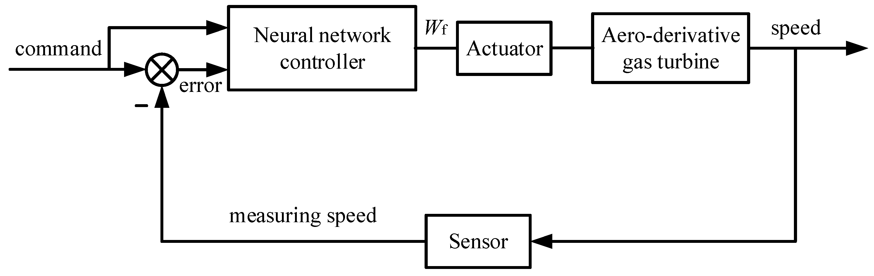
In this part, the neural network technique is employed to develop the controller, and the entire control system of the aero-derivative gas turbine is displayed in Figure 3. The inputs of the neural network controller (NNM) are speed command and speed error, and the output is the fuel flow rate.

In contrast to common neural networks, the applied network is a new neural network, called a Chebyshev polynomial, a Class 1 neural network, which is proposed by Zhang et al. [24,25], and the specific structure is given in Figure 4. There are three layers, which are the input layer, the hidden layer, and the output layer. Meanwhile, both the input layer and the output layer adopt linear activation functions. The activation function of the hidden layer adopts the Chebyshev polynomial of Class 1. For simplification, the thresholds of all the neurons are set as zero. It utilizes the weight direction determination method to obtain the optimal linking weights between the hidden layer and the output layer, only needing a step calculation, which obviously lowers the calculation time and work. Hence, this new neural network is more easily implemented by the hardware and has enormous potential in engineering application. For the neural network, the two inputs are speed command and speed error, and the output is the fuel flow rate.

In order to comprehend the new Chebyshev polynomial Class 1 neural network in depth, the working process is shown in detail. Similar to the common neural networks, it also contains a signal forward propagation process and an error back propagation process, respectively, illustrated as follows:

(1)

signal forward propagation process

The activation function of the input layer is linear, and there are two neurons. Hence, the input and output signals of the input layer, respectively, are,

$$X^{(1)}(k)=\{x_1(k),x_2(k)\}$$

(25)

$$O^{(1)}(k)=X^{(1)}(k)$$

(26)

where the superscript (1) denotes the input layer; k denotes the present time.

In the hidden layer, the input of the jth neuron is,

$$ne{t}_j^{(2)}(k)=O^{(1)}(k)$$

(27)

where the superscript (2) denotes the hidden layer.

In order to construct the activation function of the hidden layer, it firstly gives the Chebyshev polynomial of Class 1 as follows,

$$f_0(x)=1$$

(28)

$$f_1(x)=x$$

(29)

$$⋮$$

$$f_i(x)=2x{f}_{i-1}(x)-f_{i-2}(x),i=2,3,\cdots$$

(30)

Based on the above polynomial definition, the total number of hidden layer neurons is set as H = (H₁ + 1)(H₂ + 1), and the activation function of every hidden layer neuron is constructed as follows,

$$F_1(x1,x2)=f_0(x1)f_0(x2)$$

(31)

$$F_2(x1,x2)=f_0(x1)f_1(x2)$$

(32)

$$⋮$$

$$F_{H_2+1}(x1,x2)=f_0(x1)f_{H_2}(x2)$$

(33)

$$F_{H_2+2}(x1,x2)=f_1(x1)f_0(x2)$$

(34)

$$⋮$$

$$F_H(x1,x2)=f_{H_1}(x1)f_{H_2}(x2)$$

(35)

The output of the jth hidden neuron is,

$$O_j^{(2)}(k)=F_j(ne{t}_j^{(2)}(k))$$

(36)

Because the activation function of the output layer is linear, the corresponding input and output signals, respectively, are,

$$Y^{(3)}(k)={\displaystyle \sum _{j=1}^H{w}_j^{(2)}(k-1)O_j{}^{(2)}(k)}$$

(37)

$$y_m^{(3)}(k)=Y^{(3)}(k)$$

(38)

where the superscript (3) denotes the output layer; $w_j^{(2)}(k-1)$ is the linking weight between the jth hidden neuron and the output neuron at (k − 1) time.

The batch processing error function is defined as follows,

$$E(k)=\frac{1}{2}{\displaystyle \sum _{l=1}^L{(e_l(k))}^2}$$

(39)

where $e_l(k)=y_l(k)-y_m^{(3)}(k)$ is the error of the lth desired output and the network output at k time; L is the total number of sample data.

(2)

error back propagation process

In order to minimize the batch processing error function E(k), the gradient descent method needs to be adopted to revise the linking weights between the hidden layer and the output layer. The increment of the linking weight between the jth hidden neuron and the output neuron is given as follows,

$$\begin{array}{l}\Delta w_j^{(2)}(k)=-\mu \frac{\partial E(k)}{\partial w_j^{(2)}(k-1)}\\ =\mu \frac{\partial E(k)}{\partial e_l(k)}\frac{\partial e_l(k)}{\partial y_m^{(3)}(k)}\frac{\partial y_m^{(3)}(k)}{\partial Y^{(3)}(k)}\frac{\partial Y^{(3)}(k)}{\partial w_j^{(2)}(k-1)}\\ =-\mu {\displaystyle \sum _{l=1}^L[e_l(k)}{O}_j^{(2)}(k)]\end{array}$$

(40)

where μ is the learning rate, which is larger than zero.

The specific revision formula of the linking weight between the jth hidden neuron and the output neuron is,

$$w_j^{(2)}(k)=w_j^{(2)}(k-1)+\Delta w_j^{(2)}(k)$$

(41)

The training data are the Simulink model data. According to the weight direct determination method, which is proposed by Professor Zhang [24,25], the optimal linking weights between the hidden layer and the output layer can be obtained,

$$w=pinv(Z)y$$

(42)

where $w=\left[\begin{array}{c}{w}_1\\ w_2\\ ⋮\\ w_H\end{array}\right]\in R^{H\times 1}$; Z is the activated input matrix, $Z=\left[\begin{array}{cccc}{F}_1^1& F_2^1& \cdots & F_H^1\\ F_1^2& F_2^2& \cdots & F_H^2\\ ⋮& ⋮& \ddots & ⋮\\ F_1^L& F_2^L& \cdots & F_H^L\end{array}\right]\in R^{L\times H}$; $F_j^l$ is the output of the jth hidden layer neuron when the lth sample data is input to the network; y is the desired output data vector, $y=\left[\begin{array}{c}{y}_1\\ y_2\\ ⋮\\ y_L\end{array}\right]\in R^{L\times 1}$; pinv is used to calculate the pseudo inverse.

In order to determine the optimal number of hidden neurons which may exert a significant influence on the performance of the neural network, the structure determination algorithm, which is an uncertain accuracy method, is employed [24,25], and the corresponding flowchart is given in Figure 5. For the structure determination algorithm, the calculation formula of the half mean square error (HE) needs to be given as follows:

$$HE=\frac{1}{2L}{\displaystyle \sum _{l=1}^L{(y_l-y_r^{(3)})}^2}$$

(43)

The specific work process is illustrated as follows:

Step 1. Collect the sample data (x_l, y_l), l = 1, 2, …, L. Initialize the parameters including the current number of the Chebyshev polynomial of Class 1 p = 2, and the current minimal number p_min = 2. The current minimal half mean square error HE_min is set to be 10, which should be large enough so that the procedure can be smoothly actuated. In the light of the initial structure of the neural network, calculate the half mean square error HE via (43).

Step 2. If HE ≤ HE_min or p ≤ p_min + 1, proceed to step 3. Otherwise, go forward to step 5.

Step 3. According to the current structure of the neural network, calculate the activated input matrix Z, the linking weights w between the hidden layer and the output layer, and HE.

Step 4. If HE ≤ HE_min, actuated HE_min = HE, p_min = p, and w_opt = w, and allow p = p + 1, proceed to step 2. Otherwise, directly allow p = p + 1, and proceed to step 2.

Step 5. Save the minimal half mean square error HE_min, the optimal number of hidden layer neurons H_opt = p_min², and the optimal linking weights w_opt.

So far, the complete work process of this new neural network, which includes the signal forward propagation process and the error back propagation process, has been given; the calculation method of the optimal linking weights between the hidden layer and the output layer has been presented, and the structure determination algorithm has also been illustrated. In the subsequent part, the above formulas and algorithm will be employed to design and rectify the new neural network controller of the aero-derivative gas turbine.

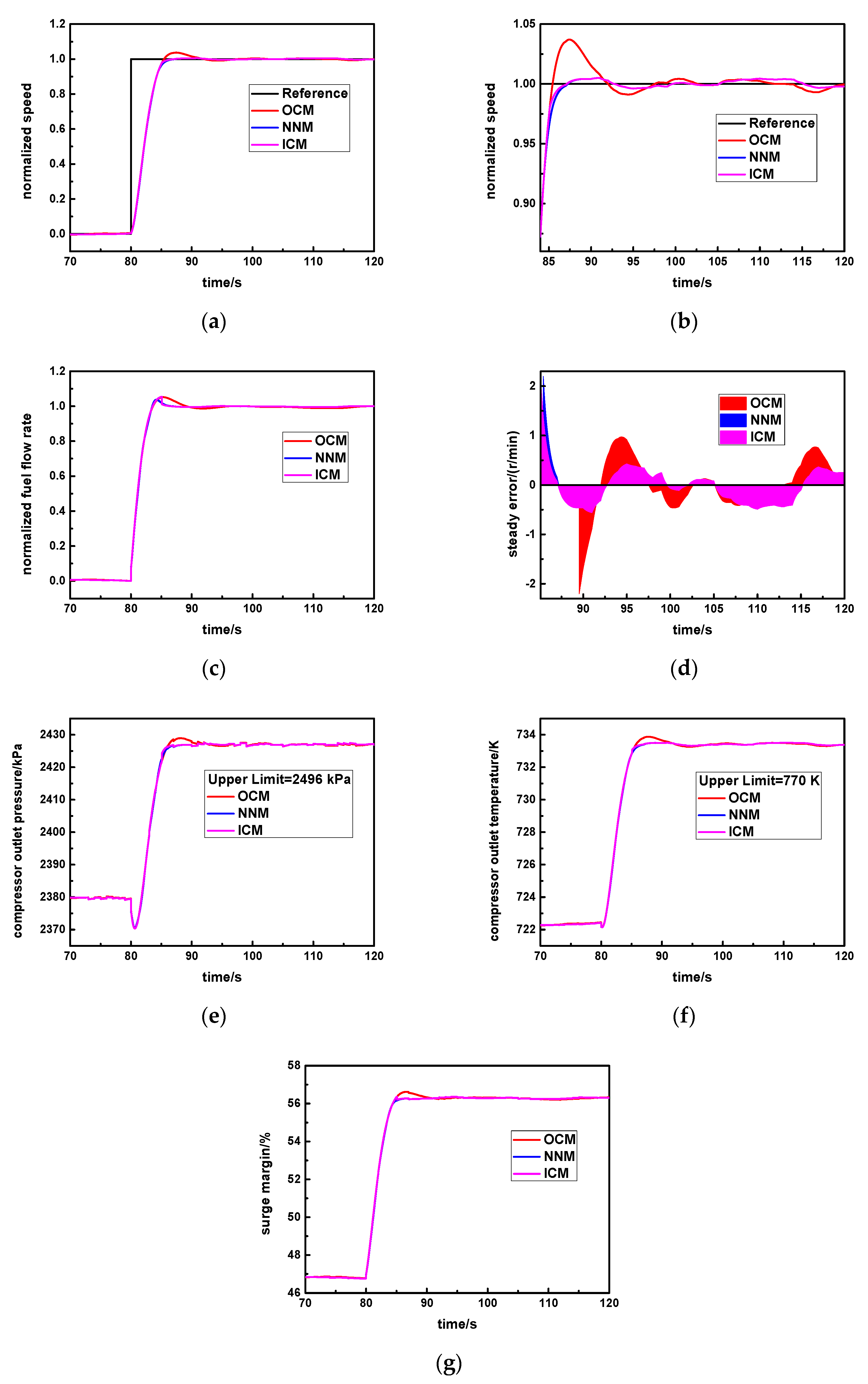
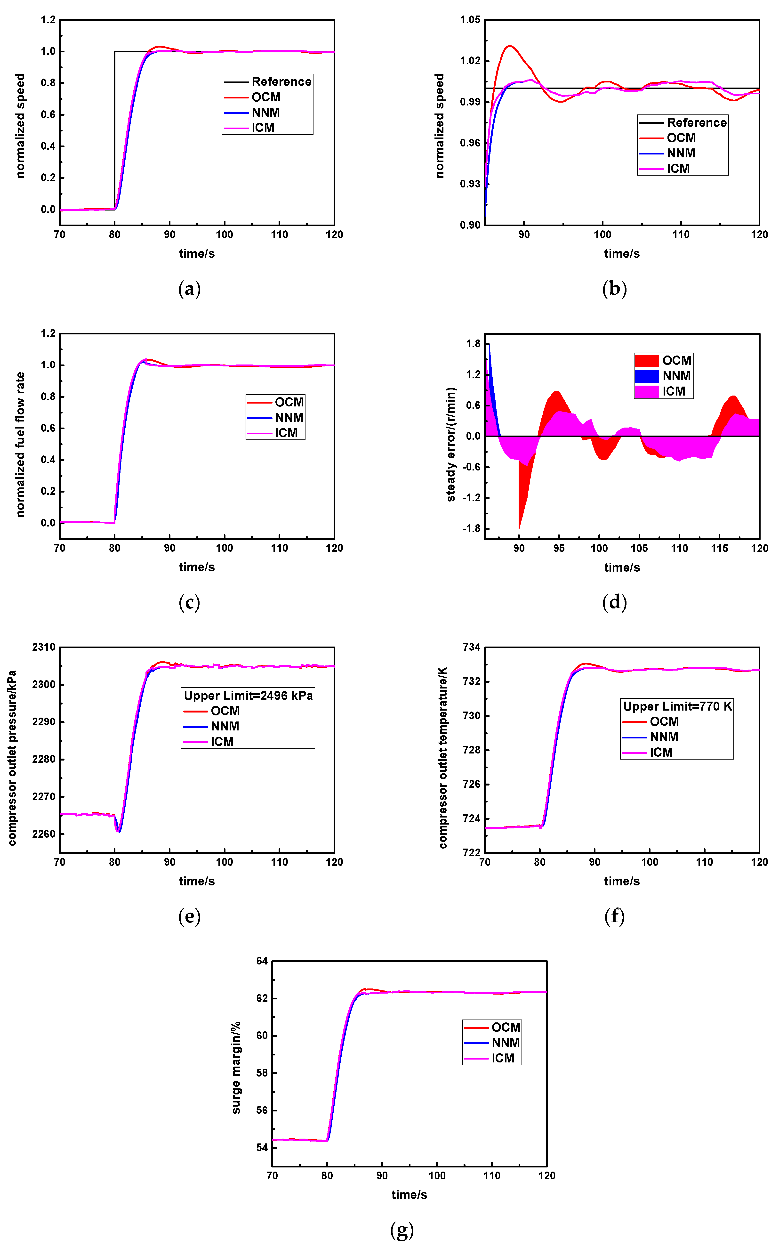
3.3. The Integrated Control Method

The original controller and a new neural network controller have been illustrated in Section 3.1 and Section 3.2, respectively. Although the original controller has a rapid response performance, the overshoot is large. Thus, the integrated control method uses the new neural network to decrease the overshoot. By combining the original controller with the new neural network controller, it develops a novel integrated control method, which is shown in Figure 6. Meanwhile, the OCM is the original controller, and the NNM is the new neural network controller. During the normal step response process, the instant error of the speed step command and the measuring speed continuously change, and the aero-derivative gas turbine will select the specific controller according to the given error threshold cv. The complete selecting logic is shown as follows:

$$SW=\{\begin{array}{l}1,error>cv\\ 2,error\le cv\end{array}$$

(44)

Specifically, cv is set as the standard steady error value. In the early response process, the instant error is larger than cv, and the original controller will be activated (SW = 1) so that response rapidity will be greater. In the steady response stage, the instant error is smaller than or equal to cv, and the new neural network controller will be triggered (SW = 2) so that it is able to obtain higher steady accuracy and avoids the larger overshoot.

In this way, the advantages of the original controller and the new neural network controller can be simultaneously utilized, which is beneficial for realizing the ideal control effect of this aero-derivative gas turbine.

The controlled variable is speed, and the controlling variable is fuel flow rate. For the neural network, the input variables are step command and speed error, and the output variable is fuel flow rate, which is the same as in Section 3.2.

4. Results and Discussion

This part takes gas generator speed as the control object to conduct the simulation test. For the purpose of verifying the performance of the proposed novel integrated control method, a tracking test and a robustness test are carried out. For one thing, because the external requirement often changes, the control system must be able to track the new command. For another, it is an indispensable characteristic that the control system also be capable of adapting to the model variation, which is induced by the parameters’ fluctuation and component performance degradation.

The above tests are carried out based on the simulation platform which is constructed by MATLAB/Simulink. The hardware conditions of the computer are Windows 10 (64 bits) operating system, 8 GB RAM, and i5-6500 CPU processor.

4.1. Model Validation

In order to validate the accuracy of the gas turbine model which is constructed by MATLAB/Simulink, the on-site data which are collected in the real test rig of the aero-derivative gas turbine are used to assess the model error. As this paper conducts research on speed control above the idle state, the validation data start to be selected from the idle condition to the design condition. The speed comparison of the dynamic process is shown in Figure 7. In addition, the relative error curve of the dynamic process is given in Figure 8.

It can be seen from Figure 7 that the maximum relative error is less than 3.723% in the initial stage; the error cause is the simplification in the bleedings’ treatment. In addition, there are many uncertainties in the real operation environment which cannot be simulated in simulation tests. However, the relative error is only −0.75% in the design stage, which meets the standard of engineering. Hence, the simulation model has satisfactory accuracy, and can be employed for the subsequent control test of the aero-derivative gas turbine.

4.2. Tracking Test

In order to evaluate the tracking performance of the novel integrated control method, after the speed attains the design speed of 9600 r/min, it carries out four step tests by setting different step commands, which are 9650, 9670, 9690 and 9710 r/min. In Section 3.3, the original controller and the new neural network controller have been abbreviated to the OCM and the NNM, respectively. In the subsequent discussions, the integrated control method is denoted as the ICM.

4.2.1. First Speed Step Test

After the speed rises to the design speed of 9600 r/min, the first speed step command of 9650 r/min is set, and it conducts the first step test. The result is given in Figure 9. The speed and fuel flow rate are normalized to the design condition. Figure 9a is the speed response curve, and Figure 9b is the locally enlarged effect. For the three control methods, their speed response curves are all able to track the step command. However, the NNM and the ICM have smaller fluctuations than the OCM. Similar to the speed response curves, the fuel flow rate variation curves of the NNM and the ICM also have smaller fluctuations, as shown in Figure 9c. It is worth mentioning that although there is an abrupt decrease in fuel flow rate for the ICM, the practical value decreases from 1.971 kg/s to 1.968 kg/s, and the decreasing percentage is only 0.152%, which does not exert an enormous effect on the fuel regulation valve.

The distribution of the steady error is illustrated in Figure 9d, where the OCM has the largest error. The variation curves of compressor outlet pressure, outlet temperature and surge margin are shown in Figure 9e–g. Meanwhile, the compressor outlet pressure and compressor outlet temperature of the three control methods do not cross the upper limit, and the surge margin is not lower than the lower limit. Therefore, the aero-derivative gas turbine is in the safe state all the time.

It can be seen from

Table 2. Tracking performance indexes of three control methods.

	Rising Time [s]	Settling Time [s]	Overshoot [%]	Error Variance
OCM	5.595	9.903	3.816	0.066
NNM	6.592	5.858	1.881	0.027
ICM	6.053	5.240	1.882	0.027

that the ICM has the shortest settling time (5.240 s), which reflects that the ICM has the rapidest response velocity and the smallest damping degree. The overshoot of the ICM is 1.882%, which is almost equal to the NNM, but obviously lower than the OCM. The steady error variance of the ICM is 0.027, which is equal to the NNM but lower than the OCM. Therefore, the ICM has a better tracking performance than the OCM and the NNM under the first step command of 9650 r/min.

4.2.2. Second Speed Step Test

As the speed attains 9600 r/min, the second speed step command of 9670 r/min is given to conduct the second step test. Figure 10a shows the speed response curve, and Figure 10b shows the locally enlarged effect. The three speed response curves can all track the step command, but the fluctuations of the NNM and the ICM are relatively weaker than the OCM. In Figure 10c, the fuel flow rate curve has a similar variation tendency to the speed response curve. Additionally, it is worth mentioning that there is a fuel flow rate step for the ICM, but the practical value decreases from 1.994 kg/s to 1.991 kg/s, and the decreasing percentage is merely 0.150%. Hence, the tiny value does not cause a tremendous impact on the fuel regulation valve.

The distribution of the steady error is displayed in Figure 10d, and the OCM has a larger error than the NNM and the ICM. In Figure 10e–g, compressor outlet pressure, outlet temperature and surge margin do not cross the allowable limits, and the safety of the aero-derivative gas turbine can be guaranteed.

From

Table 3. Tracking performance indexes of three control methods.

	Rising Time [s]	Settling Time [s]	Overshoot [%]	Error Variance
OCM	5.541	9.697	3.657	0.081
NNM	6.768	5.737	1.099	0.027
ICM	6.268	5.187	1.099	0.027

, the settling time of the ICM is the shortest (5.187 s). The overshoot of the ICM is 1.099%, which is equal to the NNM, but transparently smaller than the OCM. The steady error variance of the ICM is 0.027, which is equal to that of the NNM but smaller than that of the OCM. Overall, when the second step command of 9670 r/min is set, the tracking performance of the ICM is also the best.

4.2.3. Third Speed Step Test

After the speed increases to the design value of 9600 r/min, the third speed step command of 9690 r/min is set, and the corresponding speed response curve is displayed in Figure 11a. Similarly, the three speed response curves can all track the step command, but the speed response curves of the NNM and the ICM have smaller fluctuations than that of the OCM. The fuel flow rate curve is exhibited in Figure 11c; the variation of the NNM and the ICM is smaller than the OCM. Although there is a step for the ICM, the practical value decreases from 2.017 kg/s to 2.013 kg/s, and the decreasing percentage is barely 0.198%. Hence, this small value does not have an adverse influence on the fuel regulation valve.

In Figure 11d, the OCM has a larger steady error than the NNM and the ICM. In addition, the compressor outlet pressure, outlet temperature and surge margin are all within the allowable limits, as shown in Figure 11e–g; thus, the aero-derivative gas turbine can always operate in safe conditions.

According to

Table 4. Tracking performance indexes of three control methods.

	Rising Time [s]	Settling Time [s]	Overshoot [%]	Error Variance
OCM	5.488	9.591	3.658	0.104
NNM	6.767	5.566	0.913	0.036
ICM	6.380	5.142	0.913	0.036

, in comparison with the other two controllers, the ICM has the shortest settling time (5.142 s). The overshoot is 0.913%, which is equal to the NNM, but clearly lower than the OCM. The steady error variance of the NNM and the ICM are also the smallest (0.036), as shown in Table 4. Therefore, the proposed ICM still has the ideal tracking performance under the third step command of 9690 r/min.

4.2.4. Fourth Speed Step Test

In this part, the step command is further increased to 9710 r/min to conduct the fourth step test, after the speed attains 9600 r/min. Figure 12a shows the speed response curve. It is clear that the three response curves can all be capable of tracking the step command, and the fluctuations of the NNM and the ICM are weaker than the OCM. Figure 12c displays the fuel flow rate curve, which has the same variation as the speed curve. Although there is a decrease for the ICM, the practical value decreases from 2.040 kg/s to 2.035 kg/s, and the decreasing percentage is only 0.245%. Hence, the tiny value will not introduce an excessively negative effect on the fuel regulation valve.

In Figure 12d, the steady error of the NNM and the ICM is obviously lower than that of the OCM. Moreover, in Figure 12e–g, the compressor outlet pressure, outlet temperature and surge margin consistently stay within the safe boundaries, which can always guarantee the safety of the aero-derivative gas turbine.

It can be seen from

Table 5. Tracking performance indexes of three control methods.

	Rising Time [s]	Settling Time [s]	Overshoot [%]	Error Variance
OCM	5.436	9.537	3.740	0.134
NNM	6.778	5.417	0.739	0.049
ICM	6.485	5.100	0.739	0.049

that the settling time of the ICM is the shortest (5.100 s). The overshoot of the ICM is 0.739%, which is equal to the NNM but evidently smaller than the OCM. The steady error variance of the ICM and NNM are the smallest (0.049). In summary, as the fourth step command of 9710 r/min is set, the tracking performance of the ICM is superior to that of the OCM and the NNM.

In summary, under the four different step commands of 9650, 9670, 9690 and 9710 r/min, the integrated control method always has the best control behavior in contrast to the original controller. It shows that the ICM inherits the fast response of the OCM, utilizes the good regulation accuracy of the NNM, and makes the control performance ideal for the aero-derivative gas turbine.

4.3. Robustness Test

Besides the tracking performance, robustness is also a significant performance characteristic that should be possessed by the novel integrated control method, when the model of the aero-derivative gas turbine varies. In this part, ambient temperature and compressor performance degradation are taken into consideration to carry out three robustness tests. For one thing, when the ambient temperature changes with the season, the inlet air temperature of the compressor is different, which will change other operation parameters of the aero-derivative gas turbine. For another, gas path faults such as fouling, corrosion and erosion, etc., may cause compressor performance degradation [29,30], which will also make the operation parameters vary.

4.3.1. First Robustness Test

For this aero-derivative gas turbine, the initial ambient temperature has continuous fluctuation, and the steady value is 4 °C. When the ambient temperature increases by 5 °C, it conducts the corresponding test work to verify the robustness of the ICM by taking 9690 r/min as the step command. The speed response curve is drawn in Figure 13a, where the three speed response curves can all track the step command. It indicates that the three control methods are still able to work normally though the model of the aero-derivative gas turbine changes with the ambient temperature. However, in comparison with the OCM, the NNM and the ICM have weaker fluctuations. The fuel flow rate curve is displayed in Figure 13c and has the same variation as the speed curve.

The distribution of the steady error is illustrated in Figure 13d, where the OCM has a larger error than the NNM and the ICM. In Figure 13e–g, the compressor outlet pressure, outlet temperature and surge margin do not cross the limit; thus, the safety of the aero-derivative gas turbine can be guaranteed.

It can be seen from

Table 6. Tracking performance indexes of three control methods.

	Rising Time [s]	Settling Time [s]	Overshoot [%]	Error Variance
OCM	5.052	9.227	3.455	0.102
NNM	6.594	5.365	1.008	0.042
ICM	6.049	4.702	1.009	0.042

that the ICM has the shortest settling time (4.702 s), and the overshoot is 1.009%, which is nearly equal to the NNM but distinctly lower than the OCM. The steady error variance of the NNM and the ICM are the lowest (0.042). Hence, as the model of aero-derivative gas turbine changes with the increasing of the ambient temperature, the ICM still has an excellent tracking performance, which indicates that the ICM has the strongest robustness among the three control methods.

4.3.2. Second Robustness Test

Similarly, when compressor efficiency decreases by 2% on account of gas path faults, the speed response curve depicted in Figure 14a shows the three curves are still capable of tracking the step command, which implies that the three control methods can play their normal roles, although the model of the aero-derivative gas turbine varies with compressor efficiency. Comparatively speaking, the fluctuation of the NNM and the ICM is smaller than that of the OCM. The fuel flow rate curve is exhibited in Figure 14c.

The distribution of the steady error is given in Figure 14d, and the error of the NNM and the ICM is smaller than that of the OCM. Additionally, in Figure 14e–g, the compressor outlet pressure, outlet temperature and the surge margin of the three control methods are all within the allowable limits, which can guarantee the safety of the aero-derivative gas turbine.

It can be seen in

Table 7. Tracking performance indexes of three control methods.

	Rising Time [s]	Settling Time [s]	Overshoot [%]	Error Variance
OCM	6.171	9.993	3.194	0.110
NNM	7.313	6.307	0.995	0.040
ICM	7.014	5.748	0.998	0.040

that the settling time of the ICM is the shortest (5.748 s), and the overshoot of the ICM is 0.998%, which is slightly larger than the NNM but visibly smaller than the OCM. The steady error variance of the ICM is 0.040, which is lower than the OCM. Therefore, as the decreasing efficiency of the compressor changes the model of the aero-derivative gas turbine, the tracking performance of the ICM is still impressive, which implies that the robustness of the ICM is the best among the three control methods.

4.3.3. Third Robustness Test

When compressor efficiency decreases by 2% and the air flow rate decreases by 7%, it carries out the step test by setting a step command at 9720 r/min. The speed response curve is depicted in Figure 15a; the three curves are still capable of tracking the step command, which implies that the three control methods can play their normal role, although the model of the aero-derivative gas turbine varies with compressor efficiency and the air flow rate. Comparatively speaking, the fluctuations of the NNM and the ICM are smaller than that of the OCM. Figure 15c gives the fuel flow rate curve.

The distribution of the steady error is given in Figure 15d, and the error of the NNM and the ICM is smaller than that of the OCM. Additionally, in Figure 15e–g, the compressor outlet pressure, outlet temperature and the surge margin of the three control methods all stay within the safe limits; thus, the aero-derivative gas turbine is consistently within safe conditions.

It can be seen in

Table 8. Tracking performance indexes of three control methods.

	Rising Time [s]	Settling Time [s]	Overshoot [%]	Error Variance
OCM	4.359	6.120	2.311	0.153
NNM	5.324	4.277	0.618	0.042
ICM	5.143	4.062	0.618	0.033

that the settling time of the ICM is the shortest (4.062 s), and the overshoot of the ICM is 0.618%, which is equal to the NNM but visibly smaller than that of the OCM. The steady error variance of the ICM is the lowest (0.033). Therefore, when decreasing compressor efficiency and air flow rate change the model of the aero-derivative gas turbine, the tracking performance of the ICM is still impressive, which implies that the robustness of the ICM is the best among the three control methods.

5. Conclusions

This paper selects the speed control of an aero-derivative gas turbine as the research object and proposes a novel integrated control method based on its original controller and a new neural network controller. Aiming at gas generator speed control, the tracking test and robustness test are conducted. The corresponding conclusions have been made as follows:

(1)

During the four speed step tests, the novel integrated control method has an excellent tracking performance, with not only the shortest settling time but also the lowest steady error variance. Simultaneously, the safety of the gas turbine can also be guaranteed.

(2)

When the aero-derivative gas turbine model changes with the ambient temperature and compressor performance degradation, the novel integrated control method has stronger robustness than the other two controllers, and the safety limit is not consistently broken.

(3)

Indeed, the proposed novel integrated control method decreases the overshoot, improves the steady accuracy, and simultaneously guarantees the safety of the aero-derivative gas turbine. The research aim of this paper has been attained. This current work can lay the beneficial foundation for controller up-grading and the optimization of aero-derivative gas turbines, and even other types of gas turbine engines.

References

1. Zhao, D.; Wang, Y.; Liang, D.; Ivanov, M. Performances of regression model and artificial neural network in monitoring welding quality based on power signal. J. Mater. Res. Technol. 2020, 9, 1231–1240. [Google Scholar] [CrossRef]
2. Xie, C.; Wang, J.; Li, H.; Wan, M.; Chen, S. Spatial artificial neural network model for subgrid-scale stress and heat flux of compressible turbulence. Theor. Appl. Mech. Lett. 2020, 10, 27–32. [Google Scholar] [CrossRef]
3. Available online: https://new.siemens.com/global/en/company/stories/research-technologies/artificial-intelligence/artificial-intelligence-ai-in-gas-turbines.html (accessed on 27 June 2018).
4. Sisworahardjo, N.; El-Sharkh, M.; Alam, M. Neural network controller for microturbine power plants. Electr. Power Syst. Res. 2008, 78, 1378–1384. [Google Scholar] [CrossRef]
5. Balamurugan, S.; Xavier, R.J.; Jeyakumar, A.E. ANN controller for heavy duty gas turbine plant. Int. J. Appl. Eng. Res. 2008, 3, 1765–1771. [Google Scholar]
6. Mai, N.H. A neural control of the parallel gas turbine with differential link. In Proceedings of the International Conference on System Science and Engineering, Ho Chi Minh City, Vietnam, 21–23 July 2017; pp. 89–94. [Google Scholar]
7. Huang, Y.; Jiang, H. Neurocontrol of single shaft heavy-duty gas turbine using adaptive dynamic programming. In Proceedings of the IEEE International Joint Conference on Neural Networks, Killarney, Ireland, 12–17 July 2015. [Google Scholar]
8. Schaefer, A.M.; Schneegass, D.; Sterzing, V.; Udluft, S. A neural reinforcement learning approach to gas turbine control. In Proceedings of the IEEE International Joint Conference on Neural Networks, Orlando, FL, USA, 12–17 August 2007; Volumes 1–6; pp. 1691–1696. [Google Scholar]
9. Balamurugan, S.; Xavier, R.J.; Jeyakumar, A.E. Control of Heavy-duty Gas Turbine Plants for Parallel Operation Using Soft Computing Techniques. Electr. Power Compon. Syst. 2009, 37, 1275–1287. [Google Scholar] [CrossRef]
10. Kurd, Z.; Kelly, T.P. Using safety critical artificial neural networks in gas turbine aero-engine control. In Proceedings of the Computer Safety, Reliability, and Security, Fredrikstad, Norway, 28–30 September 2005; Volume 3688, pp. 136–150. [Google Scholar]
11. Lahroodi, M.; Mozafari, A.A. Combination of neural networks and state vector feedback adaptive control (SVFAC) technique to control the gas turbine combustor. In Proceedings of the ASME International Mechanical Engineering Congress and Exposition, Chicago, IL, USA, 5–10 November 2006. [Google Scholar]
12. Yang, B.; Wang, X. A neural network adaptive controller considering expert system for aero-engine. In Proceedings of the AIAA Modeling and Simulation Technologies Conference, Denver, CO, USA, 5–9 June 2017. [Google Scholar]
13. Wang, J.; Zhang, C.; Jing, Y. Adaptive PID control with BP neural network self-tuning in exhaust temperature of micro gas turbine. In Proceedings of the 3rd IEEE Conference on Industrial Electronics and Applications, Singapore, 3–5 June 2008; Volume 1–3, pp. 532–537. [Google Scholar]
14. Pan, L.; Lin, Z.; Yang, Y. The study of the neuromorphic self-tuning control system of the exhaust temperature of gas turbine by emulation. In Proceedings of the Combustion Science and Technology in Asia-Pacific Area: Today and Tomorrow, Nanjing, China, 23–26 November 2003; pp. 260–262. [Google Scholar]
15. Wang, J.; Zhang, C.; Jing, Y. Self-adaptive RBF neural network PID control in exhaust temperature of micro gas turbine. In Proceedings of the 2008 International Conference On Machine Learning and Cybernetics, Kunming, China, 12–15 July 2008; Volumes 1–7, pp. 2131–2136. [Google Scholar]
16. Zhang, T.; Huang, X.; Li, Q. The experimental study of neural network control system for a micro turbine engine. In Proceedings of the ASCC: 2009 7th Asian Control Conference, Hong Kong, China, 27–29 August 2009; Volumes 1–3, pp. 1264–1267. [Google Scholar]
17. Yan, S.; Bian, C.; Wang, Z. Microturbine control based on fuzzy neural network. In Proceedings of the 6th International Symposium on Instrumentation and Control Technology, Beijing, China, 13–15 October 2006; Volume 6357. [Google Scholar]
18. Deng, W.; Zhang, H. Fuzzy neural networks adaptive control of micro gas turbine with prediction model. In Proceedings of the 2006 IEEE International Conference on Networking, Sensing and Control, Fort Lauderdale, FL, USA, 23–25 April 2006; pp. 1053–1058. [Google Scholar]
19. Iqbal, M.M.M.; Xavier, R.J.; Kanakaraj, J. A neuro-fuzzy controller for grid-connected heavy-duty gas turbine power plants. Turk. J. Electr. Eng. Comput. Sci. 2017, 25, 2375–2387. [Google Scholar] [CrossRef]
20. El-Hosseini, M.; El Sehiemy, R.A.; Salah, A.H.; Abido, M.A. Modeling and control of an interconnected combined cycle gas turbine using fuzzy and ANFIS controllers. Electr. Eng. 2018, 100, 763–785. [Google Scholar] [CrossRef]
21. Jurado, F.; Ortega, M.; Cano, A.; Carpio, J. Neuro-fuzzy controller for gas turbine in biomass-based electric power plant. Electr. Power Syst. Res. 2002, 60, 123–135. [Google Scholar] [CrossRef]
22. Moloudi, M.; Mazinan, A.H. Controlling disturbances of islanding in a gas power plant via fuzzy-based neural network approach with a focus on load-shedding system. Complex Intell. Syst. 2019, 5, 79–89. [Google Scholar] [CrossRef] [Green Version]
23. Kim, D.H. Neuro-fuzzy tuning of PID controller for control of actual gas turbine power. In Proceedings of the IEEE International Conference on Computational Intelligence for Measurement Systems and Applications, Boston, MA, USA, 14–16 July 2004; pp. 192–197. [Google Scholar]
24. Zhang, Y.; Chen, D.; Ye, C. Toward Deep Neural Networks: WASD Neuronet Models, Algorithms, and Applications; CRC Press: Boca Raton, FL, USA, 2019. [Google Scholar]
25. Zhang, Y.; Yang, Y.; Li, W. Weights Direct Determination of Neural Networks; Sun Yat-Sen University Press: Guangzhou, China, 2010. [Google Scholar]
26. Zeng, T.; Zhang, Y.; Li, Z.; Qiu, B.; Ye, C. Predictions of USA Presidential Parties From 2021 to 2037 Using Historical Data Through Square Wave-Activated WASD Neural Network. IEEE Access 2020, 8, 56630–56640. [Google Scholar] [CrossRef]
27. Zhang, Y.; Xue, Z.; Jing, T.; Ling, Y.; Ye, C. Rough period estimation and peak prediction of stock market based on multiple sine functions extraction. In Proceedings of the 2018 International Conference on Machine Learning and Cybernetics, Chengdu, China, 15–18 July 2018; Volume 1, pp. 311–318. [Google Scholar]
28. Luo, G.; Sang, Z.; Wang, R. Numerical Methods for Aviation Gas Turbine Engine Simulation; National Defense Industry Press: Beijing, China, 2007. [Google Scholar]
29. Mohammadi, E.; Montazerigh, M. Simulation of Full and Part-Load Performance Deterioration of Industrial Two-Shaft Gas Turbine. J. Eng. Gas Turbines Power 2014, 136, 092602. [Google Scholar] [CrossRef]
30. Yang, Q.; Li, S.; Cao, Y. Full and part-load performance deterioration analysis of industrial three-shaft gas turbine based on genetic algorithm. In Proceedings of the ASME Turbo Expo: Turbine Technical Conference and Exposition, Seoul, Korea, 13–17 June 2016; Volume 6. [Google Scholar]
Figure 1. The structure of aero-derivative gas turbine.
Machines 10 00179 g001
Figure 2. The entire control system of the aero-derivative gas turbine using the original controller.
Machines 10 00179 g002
Figure 3. The entire control system of aero-derivative gas turbine using neural network controller.
Machines 10 00179 g003
Figure 4. The structure of Chebyshev polynomial of Class 1 neural network.
Machines 10 00179 g004
Figure 5. Flowchart of structure determination algorithm of Chebyshev polynomial of Class 1 neural network.
Machines 10 00179 g005
Figure 6. The integrated control method of aero-derivative gas turbine.
Machines 10 00179 g006
Figure 7. The speed comparison of on-site data and simulation data.
Machines 10 00179 g007
Figure 8. Relative error curve of on−site data and simulation data.
Machines 10 00179 g008
Figure 9. Related parameters distribution of first step test. (a) Speed response curve, (b) Locally enlarged speed curve, (c) Fuel flow rate, (d) Steady error, (e) Compressor outlet pressure, (f) Compressor outlet temperature, (g) Surge margin of compressor.
Machines 10 00179 g009aMachines 10 00179 g009b
Figure 10. Related parameters distribution of second step test. (a) Speed response curve, (b) Locally enlarged speed curve, (c) Fuel flow rate, (d) Steady error, (e) Compressor outlet pressure, (f) Compressor outlet temperature, (g) Surge margin of compressor.
Machines 10 00179 g010
Figure 11. Related parameters distribution of third step test. (a) Speed response curve, (b) Locally enlarged speed curve, (c) Fuel flow rate, (d) Steady error, (e) Compressor outlet pressure, (f) Compressor outlet temperature, (g) Surge margin of compressor.
Machines 10 00179 g011aMachines 10 00179 g011b
Figure 12. Related parameters distribution of fourth step test. (a) Speed response curve, (b) Locally enlarged speed curve, (c) Fuel flow rate, (d) Steady error, (e) Compressor outlet pressure, (f) Compressor outlet temperature, (g) Surge margin of compressor.
Machines 10 00179 g012
Figure 13. Related parameters distribution of first robustness test. (a) Speed response curve, (b) Locally enlarged speed curve, (c) Fuel flow rate curve, (d) Steady error of first robustness test, (e) Compressor outlet pressure, (f) Compressor outlet temperature, (g) Surge margin of compressor.
Machines 10 00179 g013
Figure 14. Related parameters distribution of second robustness test. (a) Speed response curve, (b) Locally enlarged speed curve, (c) Fuel flow rate curve, (d) Steady error of second robustness test, (e) Compressor outlet pressure, (f) Compressor outlet temperature, (g) Surge margin of compressor.
Machines 10 00179 g014aMachines 10 00179 g014b
Figure 15. Related parameters distribution of third robustness test. (a) Speed response curve, (b) Locally enlarged speed curve, (c) Fuel flow rate curve, (d) Steady error, (e) Compressor outlet pressure, (f) Compressor outlet temperature, (g) Surge margin of compressor.
Machines 10 00179 g015