Article

Flow Loss Analysis and Optimal Design of a Diving Tubular Pump

1
School of Civil Engineering and Communication, North China University of Water Resources and Electric Power, Zhengzhou 450045, China
2
Research Center of Fluid Machinery Engineering and Technology, Jiangsu University, Zhenjiang 212013, China
3
Hunan Neptune Pump Co., Ltd., Changsha 410100, China
*
Author to whom correspondence should be addressed.
Machines 2022, 10(3), 175; https://doi.org/10.3390/machines10030175
Submission received: 2 January 2022 / Revised: 22 February 2022 / Accepted: 23 February 2022 / Published: 25 February 2022
(This article belongs to the Special Issue Optimization and Flow Characteristics in Advanced Fluid Machinery)

Abstract

:
As important parts of underground water conveyance equipment, diving tubular pumps are widely used in various fields related to the national economy. Research and development of submersible pumps with better performance have become green goals that need to be achieved urgently in low-carbon development. This paper provides an effective approach for the enhancement of the performance of a diving tubular pump by adopting computational fluid dynamics, one-dimensional theory, and response surface methodology. First, the flow loss characteristics of the pump under several flow rate conditions are analyzed by entropy production theory, and then the impeller and guide vanes are redesigned using the traditional one-dimensional theory. Then, the surface response experimental method is used to improve pump hydraulic efficiency. The streamline angle (A) of the front cover of the impeller blade, the placement angle (B) of the middle streamline inlet, and the placement angle (C) of the rear cover flowline inlet are the response variables to optimize the design parameters of the diving tubular pump. Results show that wall entropy production and turbulent kinetic energy entropy production play the leading role in the internal flow loss of the diving tubular pump, while viscous entropy production can be ignored. The flow loss inside the impeller is mainly concentrated at the inlet and the outlet of the impeller blade, and the flow loss inside the guide vane is mainly concentrated in the area near the guide vane and the entrance of the guide vane. A, B, and C are all significant factors that affect efficiency. The order of the influencing factors from strong to weak is as follows: A2 (p = 0.000) > C (p = 0.007) = A × B (p = 0.007) > B (p = 0.023) > B2 (p = 0.066) > A × C (p = 0.094) > A (p = 0.162) > C2 (p = 0.386) > A × B (p = 0.421). The best combination of response variables after surface response test design is A = 9°, B = 31°, and C = 36°. After optimization, the pump efficiency and the head of the model pump are increased by 32.99% and 18.71%, respectively, under the design flow rate. The optimized model pump is subjected to tests, and the test data and the simulation data are in good agreement, which proves the feasibility of using the surface response method to optimize the design of the model pump.

1. Introduction

A tubular pump is a pump with a built-in motor. Because the inlet and outlet channels of the pump are in a straight line, the tubular pump is widely used in the fields of emergency drainage of mines, water lifting in large-scale water conservancy projects, water supply to high-rise buildings, and so on [1]. Due to the complex internal flow structure, the pump efficiency is usually low. With the rapid economic growth and the continuous increase in population, the problem of energy is becoming increasingly prominent. At present, the international community is trying to solve the problem of energy shortage; the excessive consumption of energy will inevitably lead to climate problems. Energy conservation and emission reduction are an important strategy to achieve the global carbon peak goal [2,3]. As general-purpose machinery, pumps are widely used in various fields related to the national economy. According to statistics, the electrical energy consumed by pumps accounts for about 20% of the world’s total power consumption. Therefore, improving the efficiency of the pump is of great significance in achieving energy saving, consumption reduction, and alleviation of energy shortages [4]. The research objects in this study are diving tubular pumps, which are widely used in municipal engineering, flood drainage, and emergency rescue in mine flooding accidents because of their high flow pumping characteristic. Due to power shortage on some emergency rescue occasions, identifying a method for its performance optimization is of great value.
It is necessary to analyze the flow loss of a pump before optimizing the design of the pump. The traditional pressure drop method has limitations regarding the calculation of the energy loss of a centrifugal pump, and it is impossible to accurately visualize the location and distribution of energy loss inside the centrifugal pumps. According to Denton [5], entropy generation is an effective method to explain the energy loss of fluid machinery. Therefore, this method can be used to analyze the internal energy loss of centrifugal pumps effectively and provide a reference for the optimal design of centrifugal pump flow components. Kock and Herwig [6] proposed an enhanced model to calculate the direct dissipation entropy generation based on the entropy generation theory. In recent years, the theory of entropy generation has been applied to the visualization of the location and distribution of energy loss in high-power mechanical pumps [7], the study of internal energy loss in multistage pumps with or without rings [8], the study of the energy loss area of the side channel pump [9], and the energy loss analysis of the large-flow fast-start self-priming centrifugal pump [10]. In addition, the theory of entropy generation has been applied to the study of energy loss in hydraulic turbines [11] and cavitation flow in cryogenic liquid submersible pumps [12]. It is an intuitive and feasible method to analyze the internal flow loss of a centrifugal pump based on the theory of entropy generation.
At present, methods such as intelligent optimization algorithms and experimental design are widely used in the optimal design of pumps. Si et al. [13] optimized the design of electronic water pumps based on orthogonal experiments and multi-island genetic algorithms (MIGA) with efficiency as the optimization goal, which increased the efficiency of the electronic water pump design operating point by 4.2%. Zhang et al. [14] combined a genetic algorithm with a three-dimensional hydraulic design (Q3DHD) and boundary vorticity diagnosis (BVF) to optimize the design of multiphase pump impellers and used experiments to verify the feasibility of the optimization method. The total pressure ratio and the isentropic efficiency of the compressor were improved. Kim et al. [15] optimized the four parameters of the shape of the front and rear cover plates of a centrifugal compressor impeller with the optimization goals of total pressure ratio and isentropic efficiency, combined with numerical simulation and hybrid multi-objective optimization algorithm, and the goal of significantly improving the isentropic efficiency and total pressure in the full range of working conditions was achieved. Although the optimal solution can be found theoretically by using intelligent optimization algorithms, the optimization cycle is long and computational resources are consumed. The use of experimental design methods can avoid the drawbacks of intelligent optimization algorithms. Hyun-Su et al. [16] optimized the impeller of the centrifugal compressor by the fluid–structure coupling approach and the response surface method, thereby improving the aerodynamic performance and structural stability of the centrifugal compressor. Shi et al. [17] adopted a multi-disciplinary optimization design method based on an approximation model to improve the comprehensive performance of an axial-flow pump, and the results show that the mass of a single blade was reduced from 0.947 to 0.848 kg (a decrease of 10.47%) and the efficiency of the design condition increased from 93.91% to 94.49% (an increase rate of 0.61%). Liu et al. [18] optimized the geometric parameters of the flow components of the multiphase pump based on the orthogonal optimization design method of five factors and four levels. The optimized multiphase pump has a more uniform internal gas volume fraction and pressure distribution, and its performance has been significantly improved. Bonaiuti et al. [19] optimized the impeller design of a centrifugal compressor based on a combination of experimental design, surface response, and multi-objective optimization algorithms. Lee et al. [20] optimized the design of the axial fan impeller based on the three-dimensional inverse problem design method and used the response surface method. After the optimization, the fan pressure increased by 28.2%. Thakkar et al. [21] presented an effective approach for sanitary centrifugal pump performance enhancement by adopting computational fluid dynamics and a response surface methodology with a multi-objective optimization algorithm; the efficiency improved by 10.15% at the design point compared to the initial pump. Nataraj et al. [22] implemented a response surface methodology complemented with CFD simulations to improve the performance of a centrifugal pump by modifying the impeller design. The total head was increased, and the power consumption was minimized with the optimized impeller parameters. Wang et al. [23] optimized a centrifugal pump impeller based on a numerical simulation, Latin hypercube sampling (LHS), a surrogate model, and a genetic algorithm. Three different surrogate models were compared, namely the RSM, kriging, and the radial basis neural network. At the design point, the RSM model predicted the highest efficiency while the optimization technique increased the efficiency by 8.34%.
It can be observed from the literature survey that most research only focuses on rotors in fluid machinery. Based on the energy loss analysis of the submersible tubular pump, this study combined computational fluid dynamics, one-dimensional theory, and response surface methods to modify the parameters of the guide vane and the impeller to improve the performance of the submersible tubular pump. Firstly, the CFD method is used to numerically simulate the hydraulic characteristic of the initial pump and the entropy analysis based on the calculation results are processed to identify the key factors that lead to hydraulic efficiency reduction. Secondly, the impeller and the guide vanes of the prototype pump are initially optimized in terms of the excellent hydraulic model. Next, the surface response method is used to carry out a multi-objective optimization design on the impeller and the space guide vane of the diving tubular pump to achieve the best performance. After that, the optimized model is manufactured to test pump performance. Finally, the reliability of the optimized design method is verified by experimental results, which provide a reference for the optimized design of diving tubular pumps.

2. Numerical Method

2.1. Flow Control Equations

The internal flow of the diving tubular pump studied in this paper is a three-dimensional incompressible turbulent flow. The flow control equation in the Cartesian coordinate system without considering the heat transfer of the fluid is [24]:
u ¯ i x i = 0
ρ u ¯ i t + ρ u ¯ i u ¯ j x j = p ¯ x i + x j ( μ u ¯ i u j τ i j ) ( i , j = 1 , 2 , 3 )
Since the number of unknowns in the governing equation is more than the number of equations, it is necessary to supplement the turbulence model to close the equations for a solution. The numerical simulation in this paper adopts the SST k-ω turbulence model with higher accuracy and reliability, and its equations are as follows [25,26,27]:
t ( ρ k ) + x i ( ρ w u i ) = x j ( Γ k k x j ) + G k Y k + S k
t ( ρ w ) + x i ( ρ w u i ) = x j ( Γ w w x j ) + G w Y w + D w + S w
where G k and G w are the production terms for k and w, respectively; Γk and Γw are the diffusion terms of k and w, respectively; Y k and Y w are the destruction terms of k and w, respectively; and D w represents the orthogonal divergent term.

2.2. Theory of Entropy Generation

The entropy generation analysis method is based on the second law of thermodynamics. It combines heat transfer and fluid mechanics to analyze energy loss and describes the irreversible conversion of high-quality energy, such as mechanical energy, to low-quality energy, such as internal energy. Diving tubular pumps will inevitably produce energy dissipation during operation; so this study uses the entropy generation analysis method to qualitatively and quantitatively analyze the energy loss of diving tubular pumps. Since entropy is a state quantity, the entropy generation and transport equation of a single-phase incompressible ideal fluid is [28]:
ρ ( s t + u s x + v s y + w s z ) = d i v ( q T ) + Φ T + Φ θ T 2
where d i v ( q T ) represents reversible heat transfer; t is for time; ρ is for density; T is the system temperature; s is the entropy generation rate; x, y, and z are coordinate components; and u, v, and w are velocity components in the Cartesian coordinate system. Φ is the viscous dissipation term of mechanical energy; Φ θ is the dissipation term generated by heat transfer due to temperature difference, and the two items on the right are the source terms, so both are positive values. The first term is the entropy generation generated by viscous dissipation, and the second term is the entropy generation generated by the heat transfer process. Reynolds averaging the Navier–Stokes equations decomposes unsteady variables into time-averaged and fluctuating terms, so the calculation of entropy generation is also divided into average term and pulsating term. Herwig [29] gave the formula for calculating entropy generation per unit volume after Reynolds time-average processing:
S P R O , D ¯ = μ T 2 ( u ¯ x ) 2 + ( v ¯ y ) 2 + ( w ¯ z ) 2 + ( u ¯ y + v ¯ x ) 2 + ( u ¯ z + w ¯ x ) 2 + ( v ¯ z + w ¯ y ) 2
where “-” represents the time-average term and S P R O , D ¯ represents the entropy generation due to viscous dissipation.
S P R O , D = μ T 2 ( u x ) 2 ¯ + ( v y ) 2 ¯ + ( w z ) 2 ¯ + ( u y + v x ) 2 ¯ + ( u z + w x ) 2 ¯ + ( v ¯ z + w y ) 2 ¯
where “′“ represents the pulsation term and S P R O , D represents the entropy generation caused by turbulent energy dissipation.
Since it is difficult to directly solve the pulsating velocity in the numerical calculation process, Herwig [30] proposed a method to directly solve the entropy generation of turbulent kinetic energy based on the turbulent energy dissipation rate. The calculation formula is as follows:
S P R O , D = ρ ε T
where ρ is the density, ε is the turbulent energy dissipation rate, and T is the system temperature.
Volume analysis of the above formula is performed in the calculation domain to obtain the viscous dissipation entropy generation and turbulent kinetic energy entropy generation of the calculation domain. The calculation formulas are [30]:
Δ S P R O , D ¯ = V S P R O , D ¯ d V
Δ S P R O , D = V S P R O , D d V
In addition, wall entropy generation cannot be ignored but because the medium is viscous, there is a large velocity gradient inside the boundary layer and the entropy generation near the wall is calculated by the viscous entropy generation formula with large errors. Therefore, Zhang [31] gave a method to calculate the entropy generation near the wall. The total wall entropy generation was calculated by dividing the area of the calculation domain wall by the entropy generation in the wall area. The calculation formula is as follows:
S P R O , W = A τ w v p T d A
where S P R O , W is the wall surface entropy generation, τ w is the wall shear stress, and v p is the average velocity of the fluid at the center of the first layer of the grid away from the wall.

3. Numerical Simulation and Optimization Potential Analysis of Internal Flow

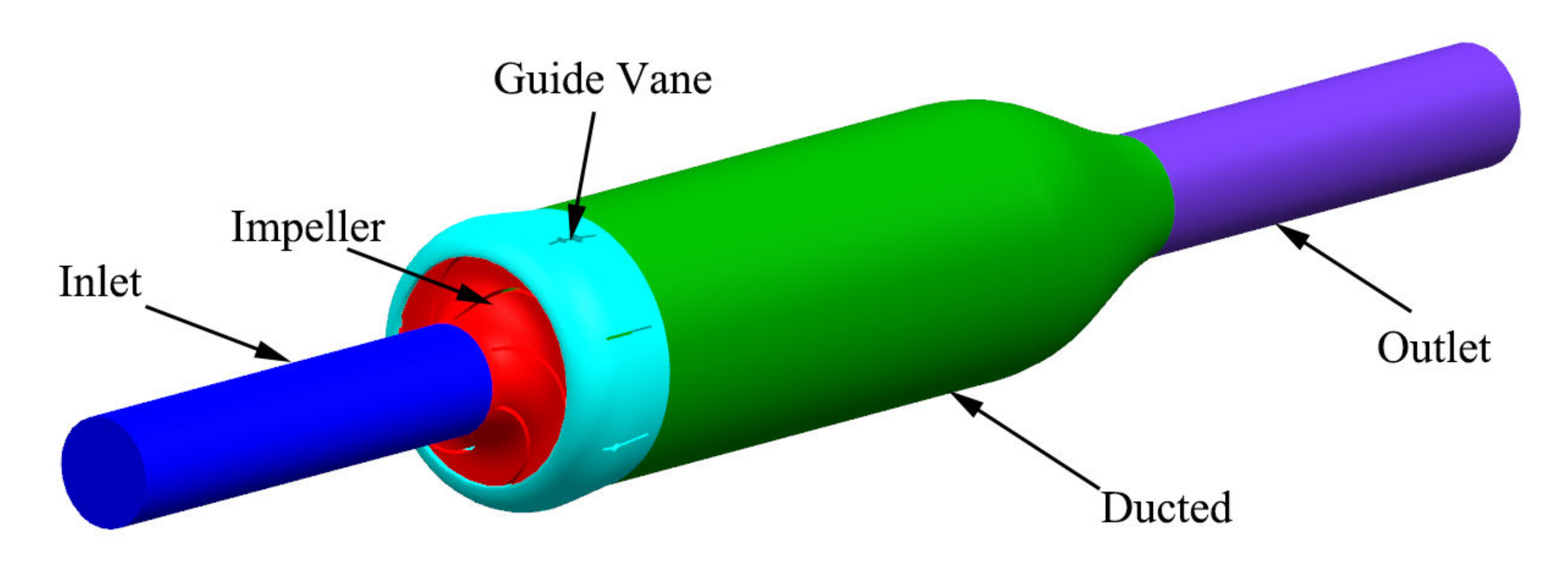
3.1. Computational Domain Model

This paper takes a diving tubular pump as the optimization object, and its main performance design parameters are shown in Table 1.
To conduct a preliminary analysis of the hydraulic performance of the diving tubular pump, three-dimensional modeling of the water body is built as the computational domain of the diving tubular pump. As shown in Figure 1, the computational domain is composed of five parts: the inlet pipe, the impeller, the spatial guide vane, the ducted, and the outlet pipe.

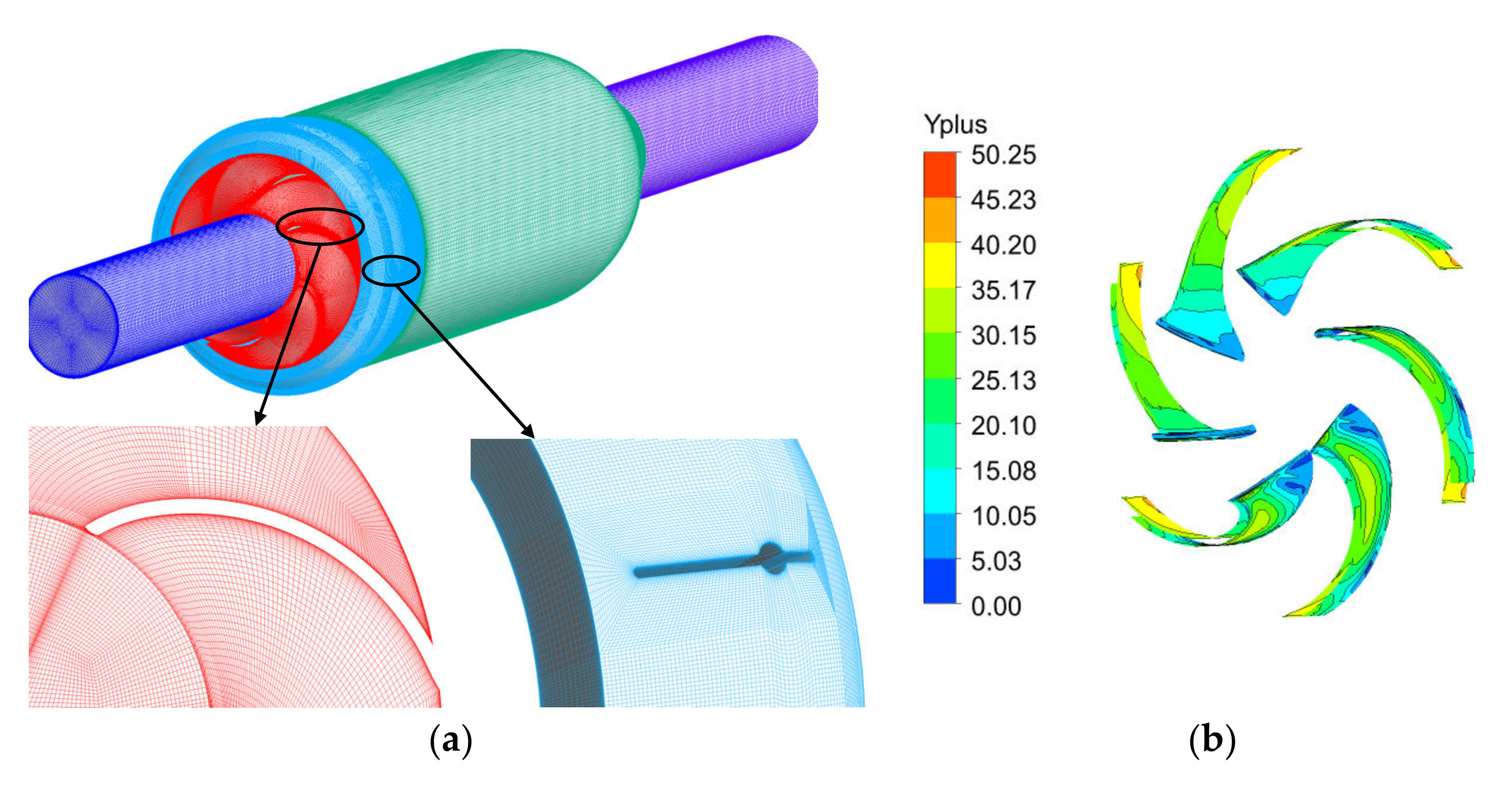
3.2. Grid Division of a Computational Domain

To improve the calculation accuracy and speed up the convergence speed, ANSYS ICEM was used to divide the water body in the calculation domain of the diving tubular pump with a structured grid. As the structured meshes only contained quadrilaterals or hexahedrons in this case, their topological structure was equivalent to a uniformly orthogonal mesh within a rectangular domain. Accordingly, the nodes on each layer of the mesh lines can be effectively adjusted to ensure a high quality [32]. For inlet and outlet pipes, ICEM with an O-Block strategy was adopted to discretize the domains. In addition, to be able to capture more flow details inside the diving tubular pump, the meshes closed to the wall part were locally encrypted. The quality of meshes within all computational domains was above 0.4. The mesh division result and the partial mesh enlargement are shown in Figure 2. To treat the high-velocity gradient, all near-wall surfaces were refined with prism layers. The expansion ratio of near-wall grids is 1.2. Because wall loss is directly affected by the quality of the wall mesh, the boundary layer was applied to improve the quality of the wall mesh. Different models have different requirements for y+ and do not have a fixed value [33,34]. The average values of y+ of each flow passage component are listed in Figure 2b, and it is less than 50 [9]. Because the calculation results were generally satisfactory, the y+ value can be considered as appropriate in this paper.
A grid-independent check (GIC) was conducted to make sure that the simulations in the optimization process are free from errors caused by the element count. It can be seen from Table 2 that when the element count increases from 7.68 to 8.56 million, the relative error of head and efficiency are 0.04% and 0.16%. Finally, the element count of 7.68 million was used for subsequent optimizations and simulations. Pump head and efficiency are defined as below.
H = p 2 p 1 ρ g + v 2 2 v 1 2 ρ g + ( z 2 z 1 )
η = ρ g H Q P

3.3. Boundary Condition Setting

To analyze the reasons for the low efficiency of the diving tubular pump and the internal flow loss, before the optimization design, numerical calculation was completed based on the commercial CFD software ANSYS CFX. The shear stress transport (SST) k-ω model of the Reynolds time-averaged equation can usually provide satisfactory results in the analysis of the internal flow field and the separation flow in the centrifugal pump [8,35]. In the paper, the SST k–ω turbulence model is applied in the numerical simulation of the model pump. The medium is clean water under normal temperature and pressure. The inlet boundary condition is set to the total pressure inlet (1 atm), the outlet boundary condition is the mass flow outlet, and the wall boundary condition is a non-slip wall. The wall function is set to an automatic wall function, the dynamic and static interface is set to a frozen rotor model, and the convection term uses a high-resolution difference format. The timestep for the transient case was 3.33 × 10⁻⁴, which corresponds to 3° of the impeller rotation. The root mean square (RMS) residual is set to 10−5.

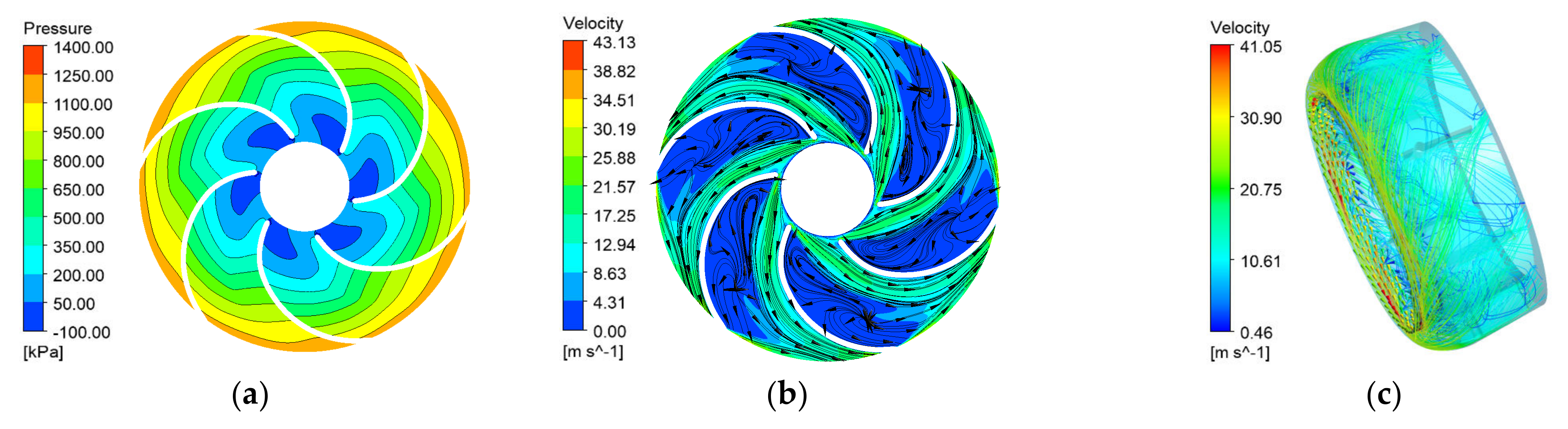
3.4. Performance Analysis of the Initial Model

To analyze the reasons for the low efficiency of diving tubular pumps, this paper determines the specific location of the internal flow loss and analyzes the cause of the flow loss according to the numerical calculation results under the design conditions. Figure 3 shows the cross-sectional pressure distribution cloud diagram, the velocity streamline diagram, and the guide vane velocity streamline diagram in the impeller under design conditions. It can be seen from Figure 3a that the pressure distribution in the inlet area of the impeller blade is uneven and the pressure at the inlet of the impeller blade fluctuates greatly. This shows that due to the unreasonable selection of the blade inlet angle, the incoming flow has a greater impact on the blade inlet edge. It can be seen from Figure 3b that there is a serious stall phenomenon on the back of the blade in the runner channel and vortices and recirculations develop on the back of the blade. It can be seen from Figure 3c that the direction of the liquid flow will change from radial to axial after the liquid flow enters the guide vane from the rotating impeller. However, since the guide vane blades of the original plan are straight, the angle of attack between the incoming flow and the inlet placement angle of the guide vane is too large. After the liquid flow enters the guide vane, there will be a large stall area and the flow state in the guide vane flow passage will show considerable disarrangement.

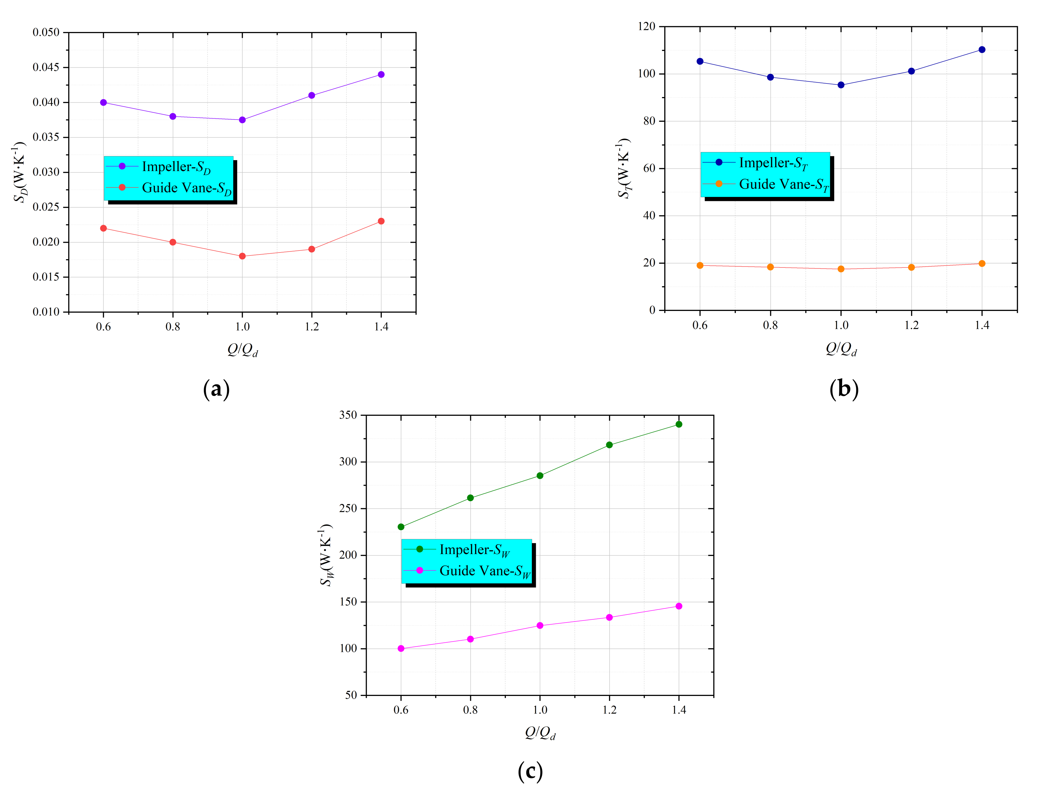
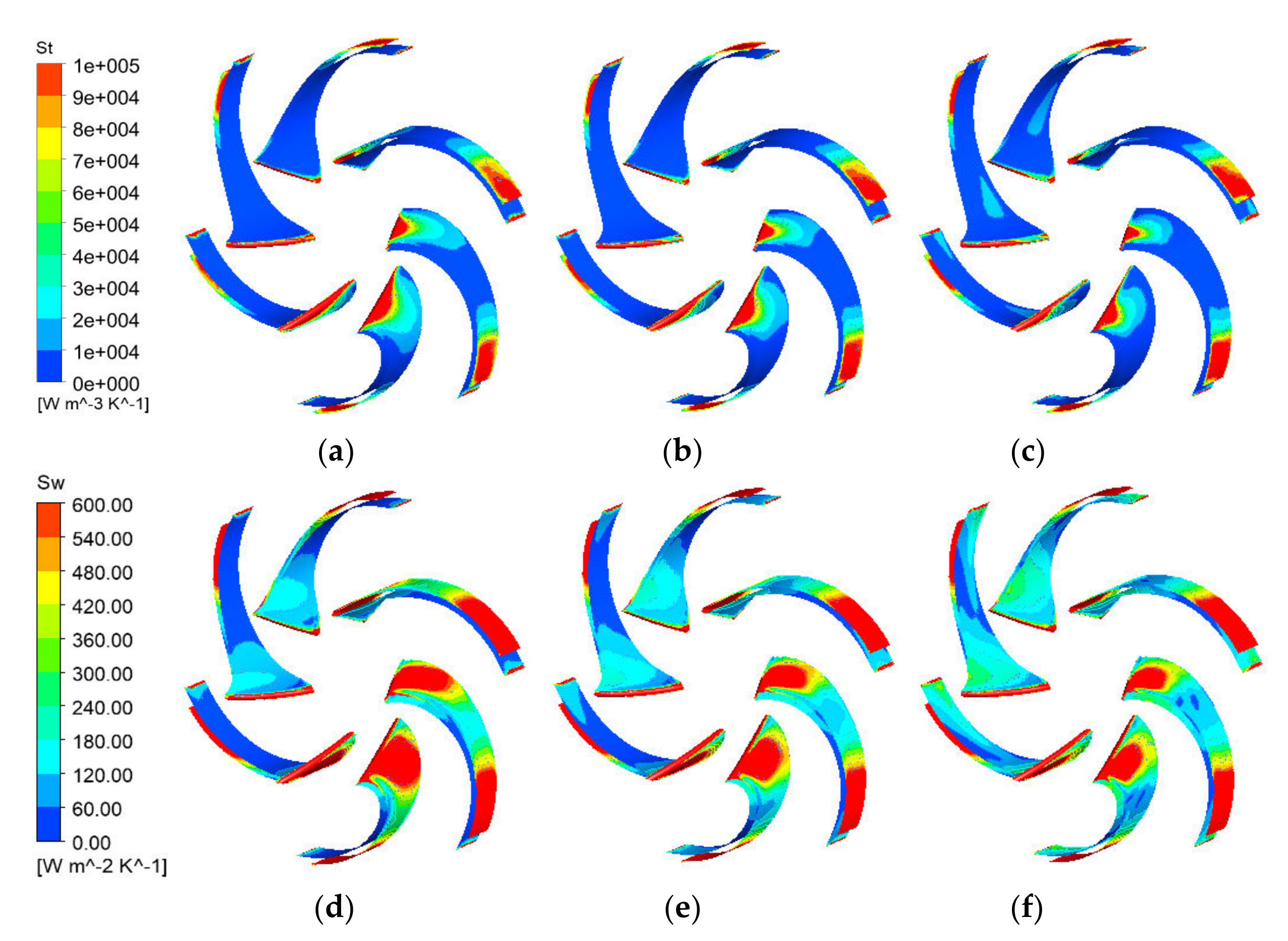
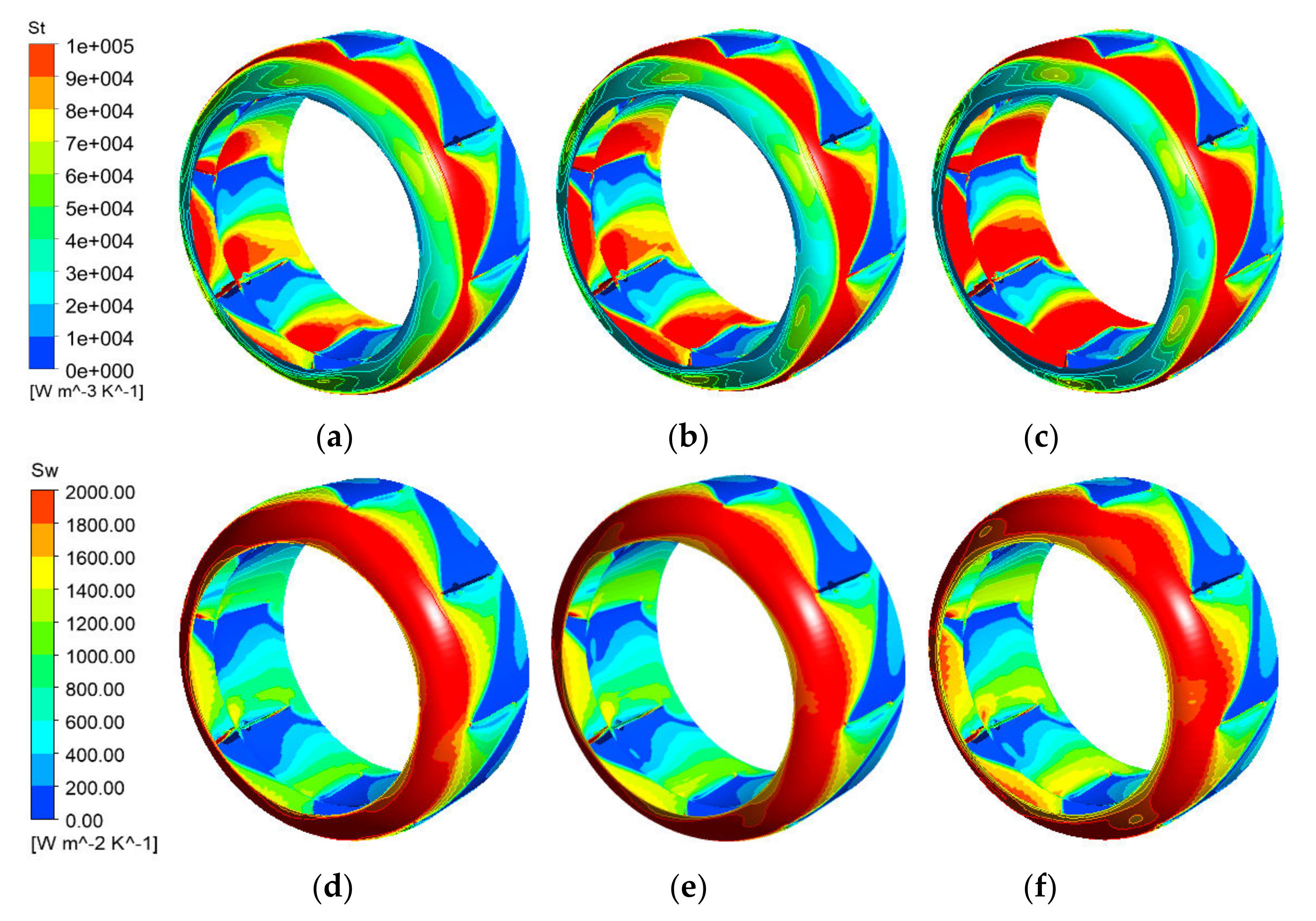
3.5. Analysis of Entropy Generation

The entropy production analysis in this paper is used to analyze the flow loss of the initial pump so as to identify the parts of the original pump with large energy loss, which provides a reference for the subsequent redesign. Figure 4 shows the entropy generation distribution of the impeller and the guide vane of the diving tubular pump. It can be seen from Figure 4 that the viscous entropy generation value and the turbulent kinetic energy entropy generation value of the impeller and the guide vane first decrease and then increase with the increase in the flow, while the wall entropy generation value increases with the increase in the flow. At the same flow rate, in terms of viscous entropy generation value, turbulent kinetic energy entropy generation value, and wall entropy generation value, the values corresponding to the guide vanes are all greater than the values corresponding to the impeller, which shows that the turbulent energy dissipation in the flow field inside the guide vane is more serious than the turbulent energy dissipation in the impeller. Under different flow conditions, the wall entropy generation value of both impeller and guide vane is greater than the entropy generation value of turbulent kinetic energy and the magnitude of wall entropy generation and turbulent kinetic energy entropy generation is much larger than the viscous entropy generation value. Therefore, the effect of viscous dissipation and entropy generation on the flow loss of diving tubular pumps can be ignored. Wall entropy generation and turbulent kinetic energy entropy generation play a leading role in the flow loss of diving tubular pumps. The subsequent analysis also mainly focuses on wall entropy generation and turbulent kinetic energy entropy generation.
Figure 5 shows the entropy generation distribution of turbulent kinetic energy and wall entropy generation on the blade surface and the guide vane surface. It can be seen that there is turbulent kinetic energy entropy generation and wall entropy generation in the blade inlet area and the blade outlet area under the three flow conditions and the entropy generation is mainly concentrated on the blade working surface. The entropy production at the blade inlet indicates that the incoming flow has an impact on the blade inlet, which results in flow loss, and the entropy generation at the blade exit is caused by the dynamic and static interference between the impeller and the guide vane. Therefore, the flow loss inside the impeller is mainly concentrated in the inlet and outlet areas of the impeller. It can also be seen from Figure 6 that there is turbulent kinetic energy entropy generation and wall entropy generation in the guide vane inlet area under the three flow conditions. The strength of the guide vane entropy generation and the area size of the generated area increase with the increased inflow. The entropy production of turbulent kinetic energy is mainly concentrated in the inlet area of the guide vane, while the wall entropy production is mainly concentrated in the inlet area of the guide vane, and the intensity of the two entropies along the axial direction shows a decreasing trend. So the internal flow loss of the guide vane is mainly concentrated in the guide vane inlet area and the guide vane blade inlet area.
From the numerical calculation results above, it can be seen that due to the deviation in the selection of the impeller blade inlet angle and the unreasonable design of the guide vane structure, the matching of the impeller and the space guide vane is problematic, which leads to large flow losses and low operating efficiency of the diving tubular pump. Therefore, this paper intends to first redesign the impeller and guide vane shape according to the excellent hydraulic model without changing the size of the impeller and guide vane axial surface. Then, based on the full-factor design of the experiment and the response surface method, the impeller blade inlet angle is used as the design variable and the efficiency and head are used as the response to perform the initial optimization of the impeller. Finally, the geometric parameters of the impeller and guide vanes that meet the expected goals are determined to achieve the improvement of the overall performance of the diving tubular pump.

4. Optimal Design

4.1. Optimal Design Based on the Empirical Method

4.1.1. Hydraulic Design of the Impeller and Guide Vanes

The impeller is designed by the empirical method [36]. Based on the traditional one-dimensional theory, the impeller is redesigned hydraulically by referring to the excellent hydraulic model of the same specific speed based on the prototype pump impeller. Same as the hydraulic design of the impeller, based on the prototype pump guide vane, the guide vane is redesigned according to the excellent hydraulic model with the same specific speed. First, the straight guide vane of the prototype pump is designed as a twisted blade and the outlet angle of the guide vane is 90°. Then, the area of the inlet of the guide vane is reduced to shift the maximum efficiency point of the diving tubular pump to the design working condition point. The research results of the literature [37,38] show that the extension of the outlet edge of the guide vane can inhibit the evolution and growth of the vortex core due to the stall, thereby improving the liquid flow in the guide vane channel. In addition, the extension of the outlet edge of the guide vane increases the static pressure of each section at the outlet of the guide vane, which can improve the rectification ability of the guide vane. The geometric parameters of the redesigned impeller and guide vanes are shown in Table 3.

4.1.2. The Results of Numerical Calculation

To compare and analyze the performance of the prototype pump, the optimized model adopts the same meshing method and the same boundary conditions as the prototype pump. Numerical calculations are completed also in ANSYS CFX. The calculation results of the pump performance are shown in Table 4. It can be seen that the optimal working condition point is at its design point, and the head of the design point is 134.59 m, which meets the design requirements. The subsequent optimization does not need to consider the head.

4.2. Optimal Design Based on the Full-Factorial Experiment

4.2.1. Optimization Object

Based on the hydraulic design of the impeller and the guide vanes in Section 4.1, the design is optimized only for the hydraulic performance of the impeller. With the streamline placement angle (A) of the front cover of the impeller blade, the placement angle (B) of the middle streamline inlet, and the placement angle (C) of the rear cover flowline inlet as the response variables and efficiency as the target variable, multi-objective optimization of the impeller of the mining pump is carried out to optimize the efficiency under the condition of meeting the head. Minitab software is used for a linearity test (full-factorial experiment) and a secondary test (response surface experiments) in this paper.

4.2.2. Full-Factor Design of the Experiment

A full-factorial experimental design is an experimental design in which all combinations of all factors and all levels must be tested at least once. Since all combinations are included, the full-factor experiment requires more time, but its advantage is that all main effects and interaction effects of various orders can be estimated. So the factorial experimental design is suitable for situations where the number of factors is small and the interaction effects of each order need to be investigated. In the full-factorial experiment design, the streamline placement angle (A) of the front cover of the impeller blade, the placement angle (B) of the middle flowline inlet, and the placement angle (C) of the back cover flowline inlet are selected as the three factors of the full-factorial experiment design factor. The level of each factor is shown in Table 5. In the table, −1, 0, and 1, respectively, represent the low level, the medium level, and the high level of the experimental factors.
Since the full-factorial experiment with three factors and two levels requires at least 8 experiments (under the condition of no repeatability test), three center points are added during optimization to reduce the error of fitting the regression equation, so a total of 11 full-factorial experiments are set. The experiment design scheme and the corresponding calculated CFD data are shown in Table 6. Analysis based on CFD calculation results and the variance of the full-factor experimental efficiency are shown in Table 7. It can be seen from the table that the p-values of A, B, and C are 0.015, 0.002, and 0.007, respectively, which means all of them are significant factors because they are less than 0.05. The order of impact factors from strong to weak is B (p = 0.002) > C (p = 0.007) > A (p = 0.015). The p-value of the two-factor interaction A * B and A * C is also less than 0.05, which also belongs to significantly affected items. The p-value of bending is 0.003, which is less than 0.005, so there is bending, indicating that the results of the linear regression equation are distorted, there is the influence of the quadratic factor, and further design experiments are needed.

4.3. Optimal Design Based on Surface Response Experimental Method

According to the results of the full-factor experimental method, the fitted bending judgment coefficient p < 0.05 (p > 0.05 proves that the model is available and no bending occurs), the equation has bending, and the main effect (single factor) coefficient p < 0.05, which proves that A, B, and C are all significant influencing factors. When the number of factors does not exceed three and they are all significant influencing factors, a more detailed surface response design analysis method should be adopted. The response surface experimental method adopts a central composite design, adding nine groups based on the full-factor experimental method. The experimental design and the corresponding experimental data are shown in Table 8.
The variance in the efficiency of the surface response experimental is shown in Table 9. It can be seen from the table that the p-values of blades A, B, and C are 0.0162, 0.023, and 0.007, respectively. The p-values of B and C are both less than 0.05, which are significant influencing factors, and the p-value of A is greater than 005, which is an insignificant influencing factor. In the square term, the p-value of A2 is 0.000, which is a strong significant influence factor, and the p-values of B2 and C2 are both greater than 0.05, which are weakly significant factors. In the two-factor interaction, the p-value of A * B is 0.007 < 0.05, and A * B is a significant influence factor, while the p-value of A * C is 0.094 and the p-value of B * C is 0.421, both greater than 0.05, which are weakly significant impact factors. It can be seen that A, B, and C are all significant factors (single term, square term, and interaction term) that affect the regression equation. The order of impact factors from strong to weak is:
A 2 P = 0.000 > C P = 0.007 = A × B P = 0.007 > B P = 0.023 > B 2 P = 0.066 > A × C P = 0.094 > A P = 0.162 > C 2 P = 0.386 > A × B P = 0.421
From the above analysis, it can be seen that the model is effective and there is no lack of fit. The multiple linear regression equation of efficiency is as follows:
η = 42.1 + 2.238 A + 0.431 B + 1.069 C 0.03316 A 2 0.00931 B 2 0.0125 C 2 0.02368 A B 0.0229 A C + 0.0089 B C
Figure 7 shows the two-factor interaction diagram of efficiency of A, B, and C. It can be seen from Figure 7a that the slopes of the curved surfaces of A and C are steep and parabolic and the efficiency value changes caused by these two factors are relatively large. When C remains unchanged, the efficiency first increases and then decreases with A. When A remains unchanged, the efficiency increases with an increase in C and the contour is presented as an ellipse with large curvature, indicating that the interaction between A and C is significant. It can be seen from Figure 7b that the influence of A and B on efficiency is more complicated. When B is at a low level, the efficiency increases with an increase in A. When A is at a low level, the efficiency increases with an increase in B. The contour lines are presented as ellipses with greater curvature. It shows that the interaction between A and C is more significant; It can be seen from Figure 7c that when C is at a low level, the efficiency decreases with an increase in B. When C is at a high level, the efficiency first increases and then decreases with an increase in B. It can also be seen from the contour lines that C and B have significant interactive effects.

4.4. Optimization Results

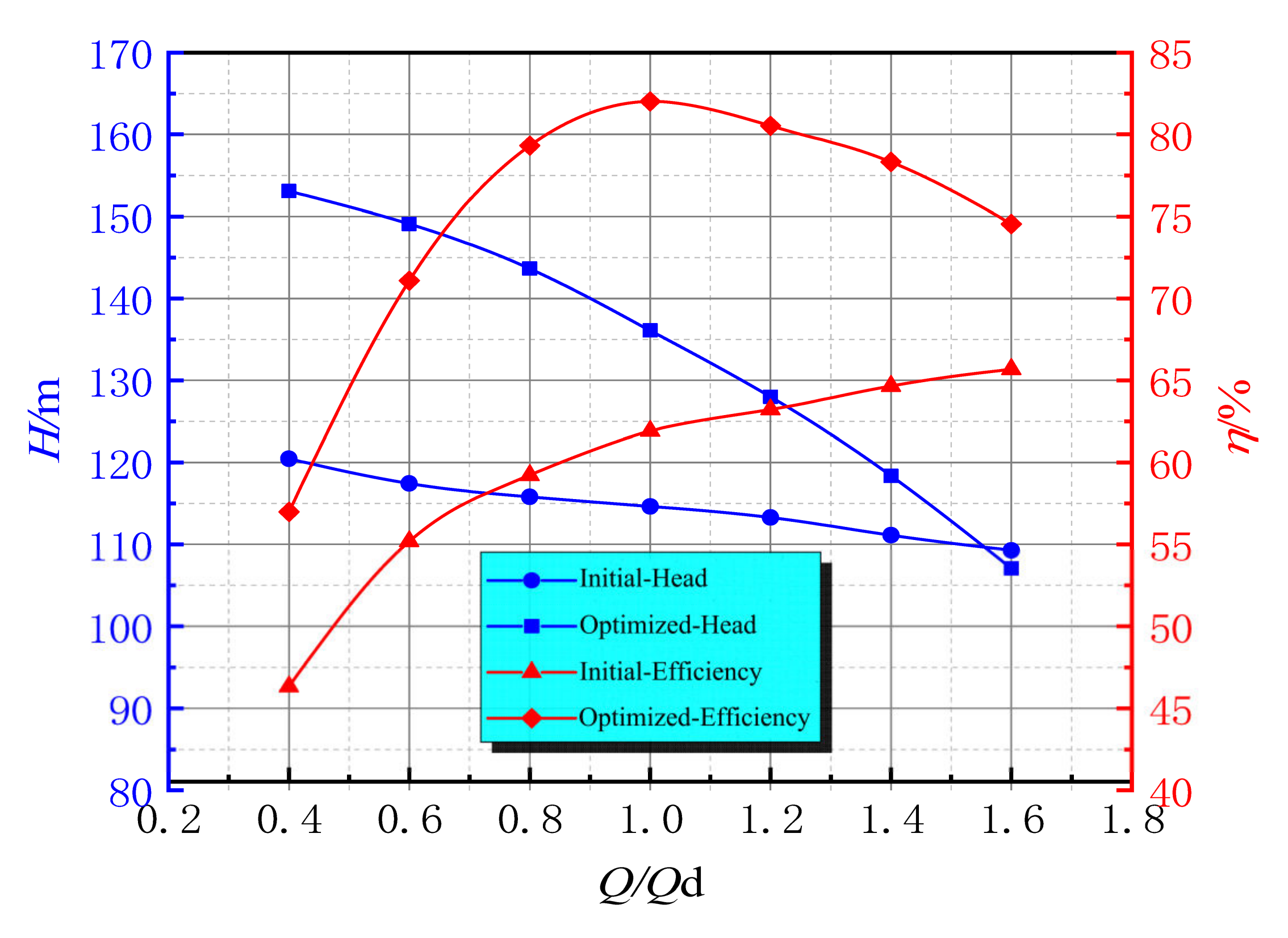
4.4.1. Comparison of Optimization Effects on Pump Performance

The optimal solutions of the response optimization variables obtained by the response optimizer are A = 10°, B = 28.87°, and C = 38.72°, and the efficiency value is 82.7%. To compare and analyze the performance of the prototype pump again, the same meshing method and the same boundary conditions are set as those of the prototype pump. The efficiency of the design operating point obtained after the numerical calculation is 81.9%, which is lower than the 82.7% obtained by the response optimizer, which is caused by the error of the fitting equation. The calculation efficiency of the 9th group in the surface response experiment design scheme is 82.34%, and the error of the efficiency value obtained by the response optimizer is only 0.435%. Therefore, the variables A = 9°, B = 31°, and C = 36° of the 9th group of experiments are selected as the best combination for solving the surface response. According to the optimal solution of the response variable, the head and efficiency values of the diving tubular pump are calculated as shown in Table 10.
To verify the accuracy of the numerical calculation results, a performance test was carried out on the model pump. Figure 8 is the schematic diagram of the pump test and the test site diagram, and it includes the tested pump, motor, pipes, multifunctional data collector, and so on. The pump was a vertical installation, and an elbow pipe was used to connect the pump and the outlet pipe. The pump outlet pressure was collected by a pressure sensor whose accuracy was better than 0.1%. The flow was measured by the electromagnetic flowmeter with an uncertainty of 0.2%, and the motor speed and other parameters were collected by a multifunctional data collector. The systematic uncertainty of the test rig was 0.36%, which meets the level 1 accuracy requirements specified in ISO9906-2012.
Figure 9 presents the optimization effect of the numerical simulation on the pump performance, and Figure 10 shows the comparison between the test and the numerical simulation after the optimization. It can be seen from Figure 9 that the head and the efficiency of the pump after optimization have been greatly improved compared with those before optimization. The efficiency improvement is most obvious near the design operating point. The performance curve has no camelback phenomenon; the efficiency curve declines slowly under large flow rate conditions, and the range of the high-efficiency zone has been broadened. In addition, the optimal working condition point of the optimized diving tubular pump efficiency is located at the design working condition (1.0Qd), with an efficiency value of 82.34% and head of 136.09 m. The efficiency of the optimized model is increased by 32.99%, and that of the head is increased by 18.71% compared with the initial scheme under design conditions, which fully meets the design requirements. The pump adopts a variable frequency motor, so the frequency converter is used to drive the pump to 3600 r/min during the engineering application. However, the frequency converter will interfere with the test sensor during the experiment. Therefore, the pump test does not use the frequency converter to drive the motor instead of the 50 Hz AC, which could drive the pump to 2900 r/min. To compare the numerical simulation and the test data, the pump flow rate and the pump head are made dimensionless as per Equation (16) and Equation (17), and the results are shown in Figure 10.
φ = Q l 2 π R 2 b 2 u 2
ψ = g H u 2 2
As the mechanical and volumetric efficiency was not considered in simulations, the results obtained by CFD are generally higher than the experimental values. It can be seen from Figure 10 that the trends of the head coefficient curve and the efficiency curve of the test and the numerical simulation are consistent with the flow rate increase. The maximum relative errors of the head coefficient and hydraulic efficiency are lower than 5%. The absolute predicted deviations for the head coefficient and hydraulic efficiency at the design condition are 2.47% and 2.92%, which proves that the optimization method and the numerical simulation method adopted in this research are correct and feasible.

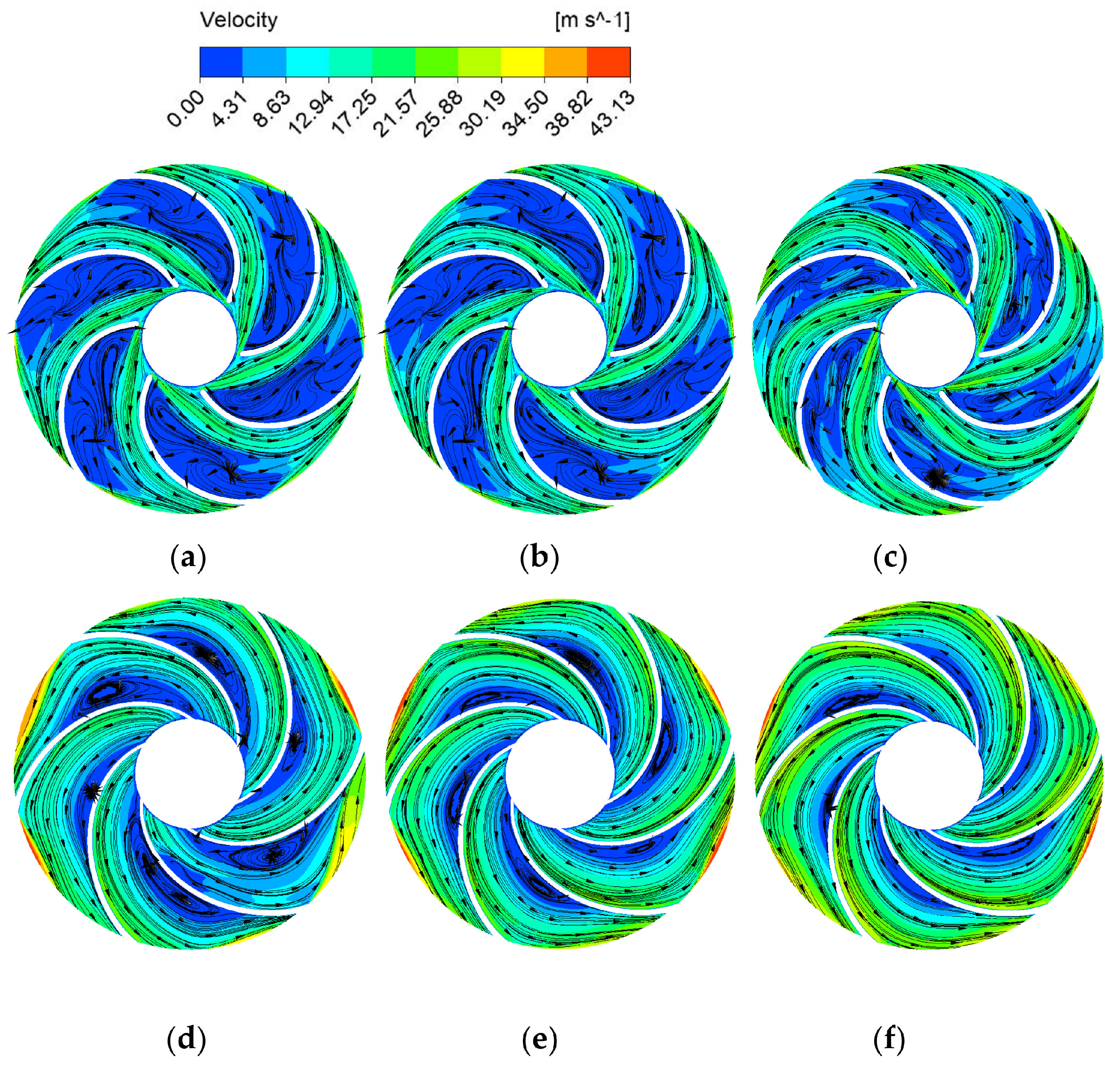
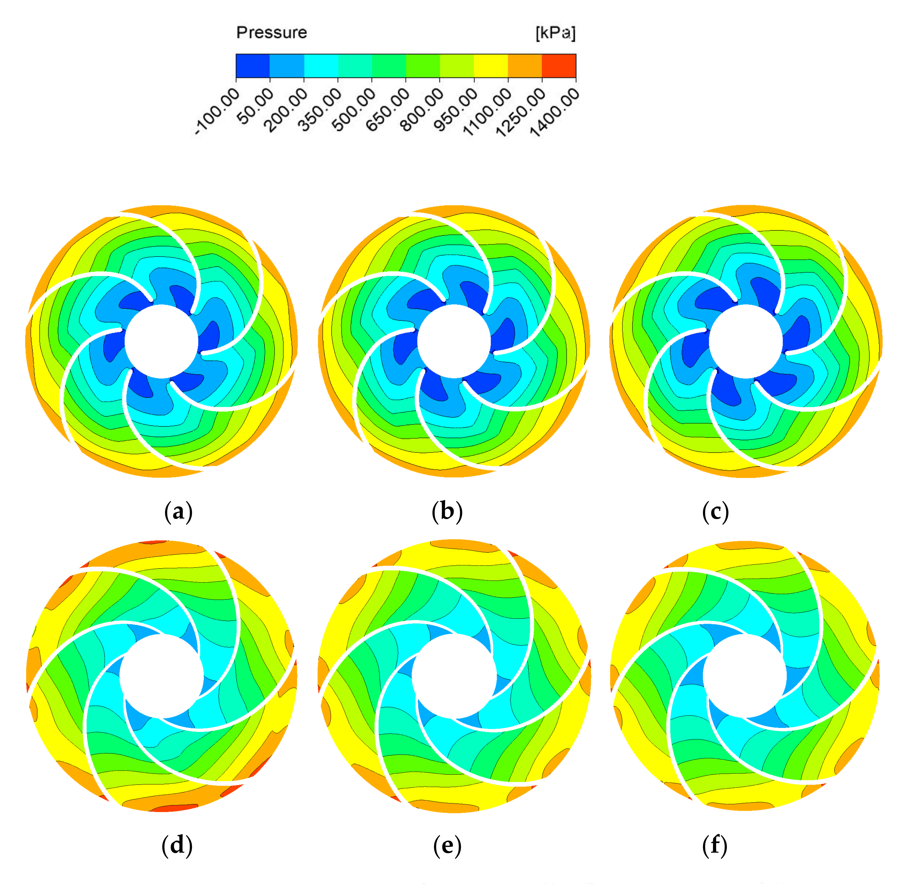
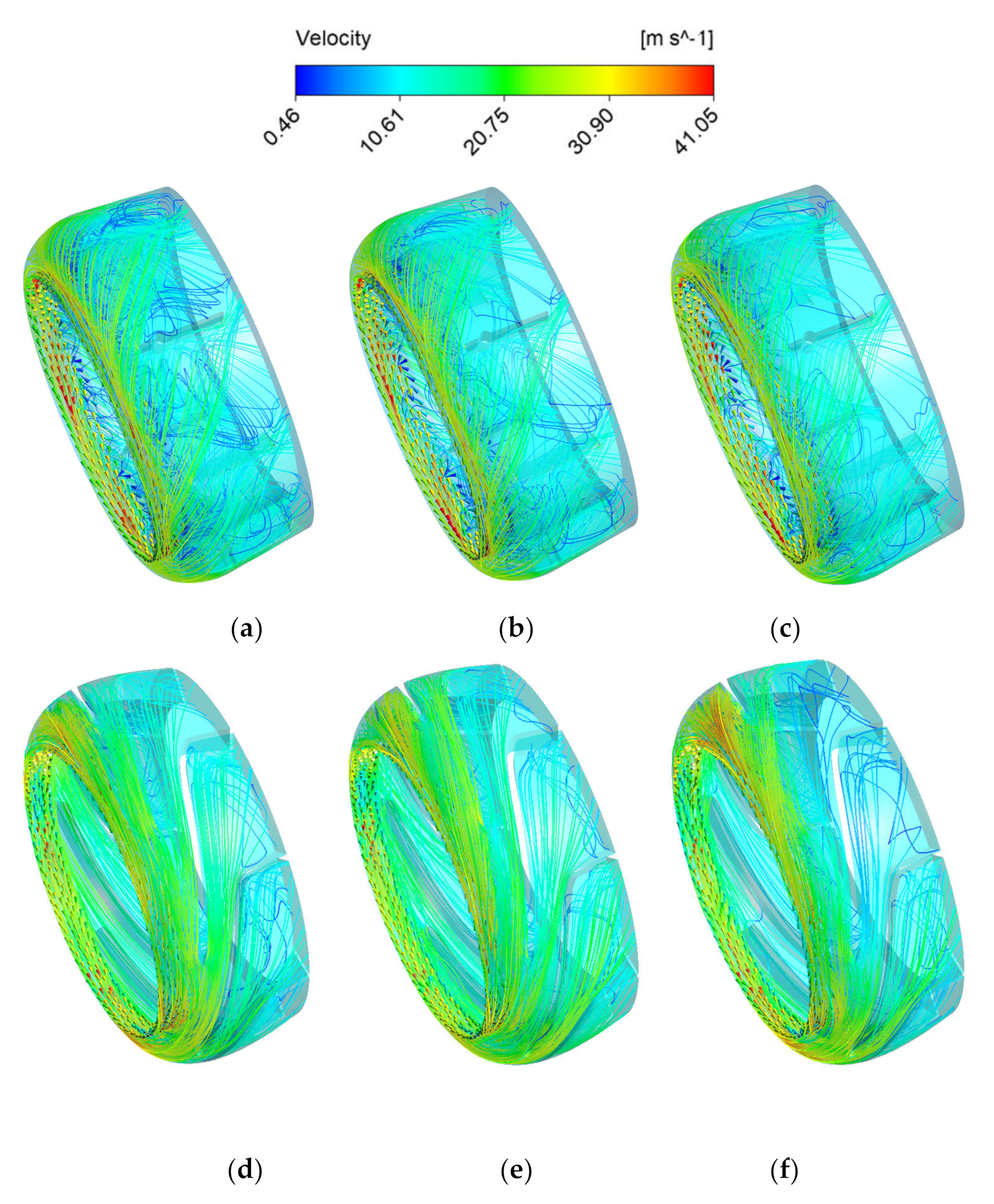
4.4.2. Analysis of Internal Flow Characteristics

Figure 11 shows the velocity streamline distribution diagram of the middle section of the impeller outlet. Before optimization, there is a large-scale separation vortex on the back of the blade and backflow occurs. The vortex area and the backflow area occupy more than half of the flow channel, and the flow pattern is turbulent. The flow velocity in the vortex area and the backflow area is low, and the velocity distribution in the entire flow channel is uneven, which leads to a reduction in the blade’s functional power, which seriously affects the hydraulic performance of the diving tubular pump. The large-scale separation vortices in the optimized impeller flow channel are significantly reduced. Only small-scale vortices are generated on the blade working surface, but there is no backflow phenomenon in the flow channel. Meanwhile, the flow velocity distribution in the flow channel after optimization is more uniform, and the vortex located on the blade working surface gradually disappears with the flow increase. Overall, the flow loss after optimization is significantly reduced compared to that before optimization, so the hydraulic performance of the diving tubular pump has been improved.
Figure 12 shows the static pressure distribution cloud diagram of the middle section of the impeller. Before optimization, there is a large low-pressure area at the blade inlet and the static pressure distribution is extremely uneven. The pressure distribution at the inlet presents a phenomenon of alternating high pressure and low pressure under different flow rates, and the low-pressure zone gradually expands with the flow rate increase. It shows that the improper setting of the blade inlet angle before optimization resulted in a serious impact between the incoming flow and the blade inlet, resulting in greater flow loss. In addition, due to the existence of a large low-pressure region, the possibility of cavitation at the blade inlet side was increased. The low-pressure region at the inlet of the optimized impeller is reduced, the static pressure at the inlet is increased compared to before optimization, and the static pressure distribution is more even. The pressure at the outlet of the impeller is reduced compared to that before optimization, so the energy loss caused by the liquid flow from the impeller into the guide vane is reduced.
Figure 13 shows the internal velocity streamline distribution diagram of the guide vane. Before optimization, the guide vane blades of the original plan were straight, resulting in an excessively large attack angle between the incoming flow and the entrance angle of the guide vane and a large area of stall occurred after the liquid flow entered the guide vane. In addition, the flow pattern in the guide vane shows disarrangement and the velocity at the inlet of the guide vane is unevenly distributed, which is more obvious under small flow conditions. After optimization, the stall area of the guide vane is significantly reduced, the streamline distribution is more uniform, and the flow pattern is improved. In addition, the flow velocity in the guide vane inlet area is stable, indicating that the selection of a reasonable guide vane inlet angle and design of the guide vane blade profile improves the internal flow of the guide vane and its internal flow loss is reduced.

5. Conclusions

Based on the theory of entropy production, the energy loss analysis of a submersible tube pump was carried out and the reasons for its low efficiency were analyzed. The investigation on the diving tubular pump with low hydraulic efficiency performance improvement was carried out with the parameters of the impeller blade and the guide vane as design variables by coupling the numerical simulation, one-dimensional theory, and response surface methodology. Three design variables, the streamline placement angle (A) of the front cover of the impeller blade, the placement angle (B) of the middle streamline inlet, and the placement angle (C) of the streamline inlet of the rear cover, with two objectives, pump head and efficiency, were considered to construct the RSM model. The reliability of the numerical simulation was validated by the experimental test. The results show that:
(1)
Entropy generation can effectively visualize the flow loss distribution caused by turbulent dissipation and flow separation. The internal flow loss of the diving tubular pump is mainly concentrated in the inlet and outlet area of the impeller and the inlet area of the guide vane. The main cause of flow loss is that the angle of attack between the relative liquid flow angle and the blade placement angle at the inlet of the impeller blade is too large; the matching between the guide vane and the impeller is poor, and the guide vane design is unreasonable.
(2)
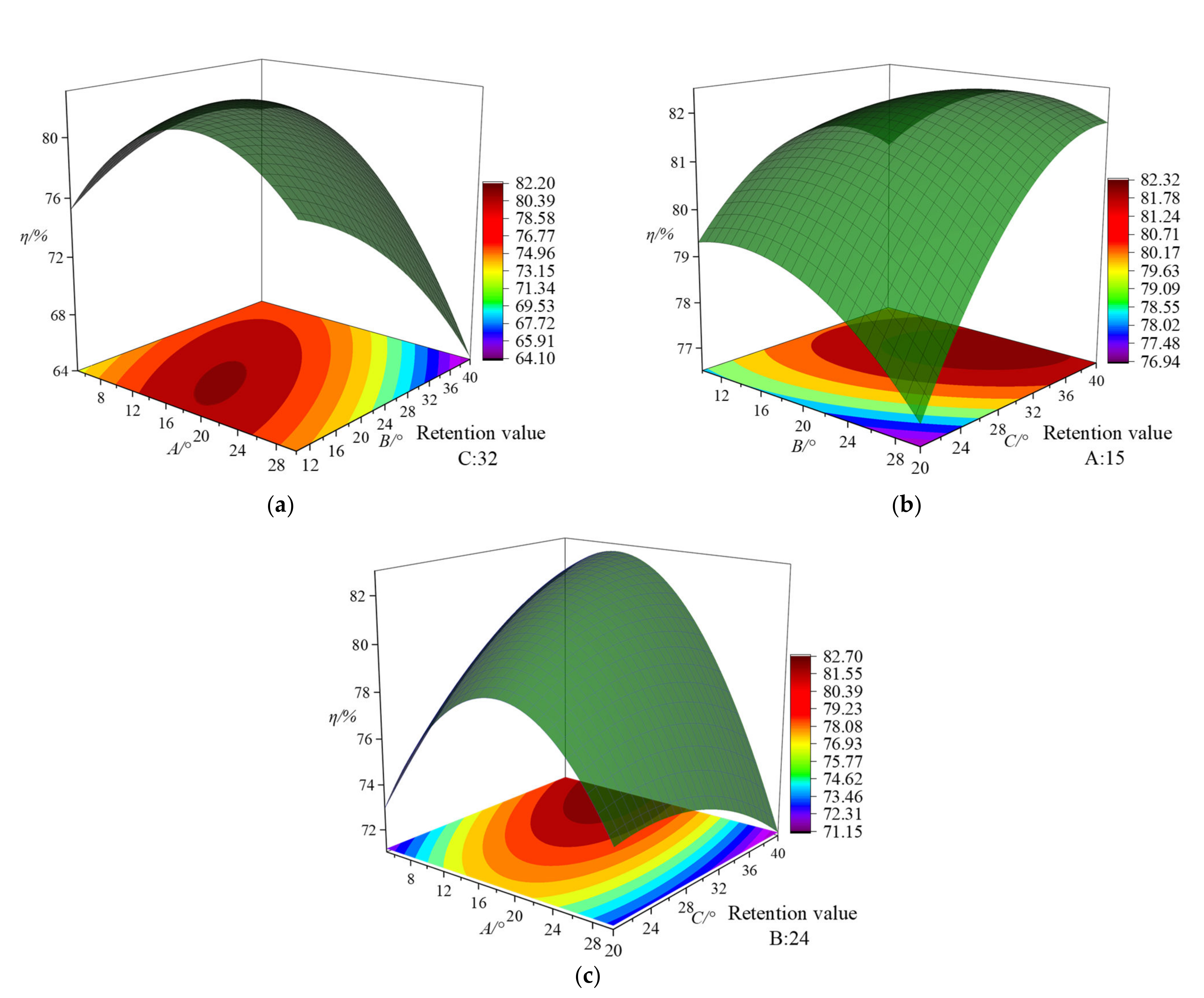
The streamline placement angle (A) of the front cover of the impeller blade, the placement angle (B) of the middle streamline inlet, and the placement angle (C) of the streamline inlet of the rear cover are all significant factors that affect the efficiency. The order of the influencing factors from strong to weak is as follows: A2 (p = 0.000) > C (p = 0.007) = A * B (p = 0.007) > B (p = 0.023) > B2 (p = 0.066) > A * C (p = 0.094) > A (p = 0.162) > C2 (p = 0.386) > A * B (p = 0.421). The best combination of response variables after surface response test design is A = 9°, B = 31°, and C = 36°.
(3)
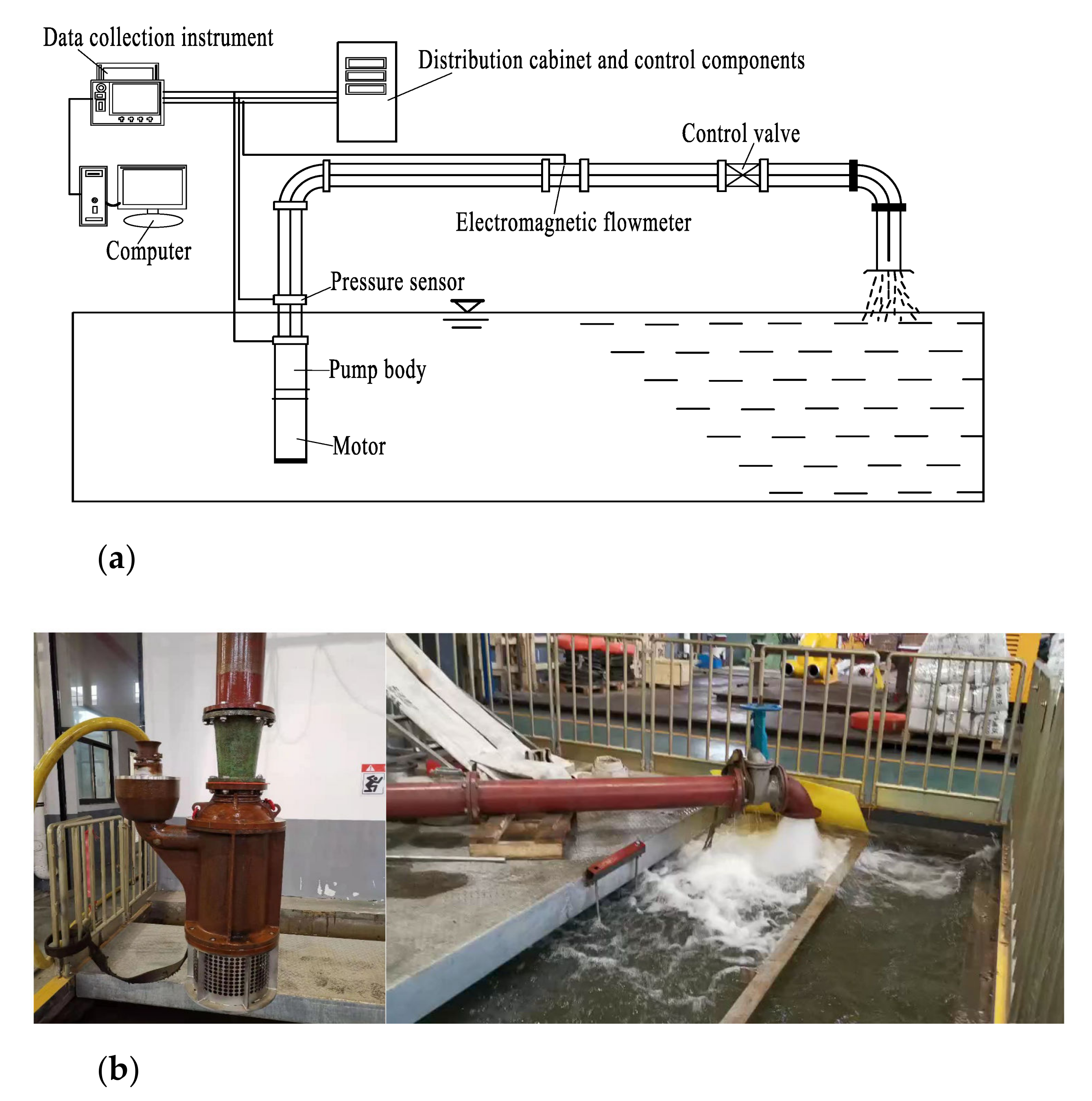
The optimization process successfully improves the head and efficiency by 32.99% and 18.71%, respectively, compared to those of the initial pump. The optimized simulation data of the diving tubular pump are in good agreement with the test data. After optimization, the large-scale separation vortex inside the impeller is significantly reduced and no backflow occurs. The internal outflow area of the guide vane is significantly reduced after optimization, and the internal flow is greatly improved because the flow is more uniform and smoother.
(4)
The optimization method in this study is universal and can be applied to conduct optimization of other fluid machinery. This study focuses on only some parameters of the impeller, and more parameters can be studied as variables in the future.

Author Contributions

Data curation, D.T.; Formal analysis, X.H.; Funding acquisition, Q.S. and Z.L.; Investigation, M.L.; Supervision, Q.S.; Validation, J.H. and Z.L.; Writing – original draft, X.Y. All authors have read and agreed to the published version of the manuscript.

Funding

This research was funded by the National Key Research and Development Program of China (No. 2020YFC1512403), the National Natural Science Foundation of China (No. 51976079), Research Project of State Key Laboratory of Mechanical System and Vibration MSV202201, and Industry University Research Cooperation Project of Jiangsu Province (No. BY2019059).

Institutional Review Board Statement

Not applicable.

Informed Consent Statement

Not applicable.

Data Availability Statement

Not applicable.

Conflicts of Interest

The authors declare no conflict of interest.

Nomenclature

u v wCartesian velocity components
x y zCoordinate components
tTime
pPressure
μDynamic viscosity
νKinematic viscosity
εTurbulent eddy dissipation
TTemperature
sEntropy
p1Pressure of the pump inlet
p2Pressure of the pump outlet
v1Velocity of the pump inlet
v2Velocity of the pump outlet
z1Installation height of the pump inlet
z2Installation height of the pump outlet
PShaft power
Φ The viscous dissipation term of mechanical energy
Φ θ The dissipation term generated by heat transfer due to temperature difference
S P R O , D ¯ Viscous entropy generation
S P R O , D Turbulent kinetic energy entropy generation
S P R O , W Wall entropy generation
τ w Wall shear stress
v p The average velocity
QRate flow
HHead
nRotational speed
ηEfficiency
DhHub diameter
DjImpeller inlet diameter
D2Impeller outlet diameter
b2Impeller outlet width
ϕ Blade wrap angle
φ2Blade outlet angle
ZBlade number
b3Guide vane inlet width
D3Maximum diameter of an inner streamline of the guide vane
D4Maximum diameter of an outer streamline of the guide vane
D5Inside diameter of the guide vane outlet
D6Outside diameter of the guide vane outlet
LAxial length of the guide vane
ZNumber of guide vanes
α3Guide vane inlet angle
α4Guide vane outlet angle
φ 0 Guide vane wrap angle
φ Flow coefficient
ψ Head coefficient
AThe streamline placement angle of the front cover of the impeller blade
BThe placement angle of the middle streamline inlet
CThe placement angle of the rear cover flowline inlet
Superscripts
-Time-averaged value
Fluctuating component

References

  1. Shi, L.J.; Zhang, W.P.; Jiao, H.F.; Tang, F.P.; Wang, L.; Sun, D.D.; Shi, W. Numerical simulation and experimental study on the comparison of the hydraulic characteristics of an axial-flow pump and a full tubular pump. Renew. Energy 2020, 153, 1455–1464. [Google Scholar] [CrossRef]
  2. Abdelaziz, E.A.; Saidur, R.; Mekhilef, S. A review on energy saving strategies in industrial sector. Renew. Sustain. Energy Rev. 2011, 15, 150–168. [Google Scholar] [CrossRef]
  3. Edwards, G.; Spence, D. The European Commission. Dev. Eur. 1997, 8, 14–26. [Google Scholar]
  4. Shankar, A.; Kalaiselvan, V.; Subramaniam, U.; Shanmugam, P.; Hanigovszki, N. A comprehensive review on energy efficiency enhancement initiatives in centrifugal pumping system. Appl. Energy 2016, 181, 495–513. [Google Scholar] [CrossRef]
  5. Denton, J.D. Loss Mechanisms in Turbomachines. Trans ASME J. Turbomach. 1993, 115, 10–23. [Google Scholar] [CrossRef]
  6. Herwig, H.; Kock, F. Direct and indirect methods of calculating entropy generation rates in turbulent convective heat transfer problems. Heat Mass Transf. 2007, 43, 207–215. [Google Scholar] [CrossRef]
  7. Gu, Y.; Pei, J.; Yuan, S.; Wang, W.; Zhang, F.; Wang, P. Clocking Effect of Vaned Diffuser on Hydraulic Performance of High-Power Pump by Using the Numerical Flow Loss Visualization Method. Energy 2019, 170, 986–997. [Google Scholar] [CrossRef]
  8. Ren, Y.; Zhu, Z.C.; Wu, D.H.; Li, X.J. Influence of guide ring on energy loss in a multistage centrifugal pump. J. Fluids Eng. 2019, 141, 0613021–06130213. [Google Scholar]
  9. Zhang, F.; Appiah, D.; Hong, F.; Zhang, J.; Wei, X. Energy loss evaluation in a side channel pump under different wrapping angles using entropy production method. Int. Commun. Heat Mass Transf. 2020, 113, 104526. [Google Scholar] [CrossRef]
  10. Hao, C.; Shi, W.D.; Li, W.; Liu, J.R. Energy loss analysis of novel self-priming pump based on the entropy production theory. J. Therm. Sci. 2019, 28, 150–162. [Google Scholar]
  11. Li, D.; Wang, H.; Qin, Y.; Han, L.; Wei, X.; Qin, D. Entropy production analysis of hysteresis characteristic of a pump-turbine model. Energy Convers. Manag. 2017, 149, 175–191. [Google Scholar] [CrossRef]
  12. Wang, C.; Zhang, Y.; Hou, H.; Zhang, J.; Xu, C. Entropy production diagnostic analysis of energy consumption for cavitation flow in a two-stage lng cryogenic submerged pump. Int. J. Heat Mass Transf. 2019, 129, 342–356. [Google Scholar] [CrossRef]
  13. Si, Q.; Lu, R.; Shen, C.; Xia, S.; Sheng, G.; Yuan, J. An intelligent cfd-based optimization system for fluid machinery: Automotive electronic pump case application. Appl. Sci. 2020, 10, 366. [Google Scholar] [CrossRef] [Green Version]
  14. Zhang, J.Y.; Cai, S.J.; Li, Y.J.; Zhou, X.; Zhang, Y.X. Optimization design of multiphase pump impeller based on combined genetic algorithm and boundary vortex flux diagnosis. J. Hydrodyn. 2017, 29, 1023–1034. [Google Scholar] [CrossRef]
  15. Kim, J.H.; Choi, J.H.; Husain, A.; Kim, K.Y. Multi-objective optimization of a centrifugal compressor impeller through evolutionary algorithms. Proc. Inst. Mech. Eng. J. Power Energy 2010, 224, 711–721. [Google Scholar] [CrossRef]
  16. Kang, H.S.; Song, Y.J.; Kim, Y.J. Optimal Design of Impeller for Centrifugal Compressor Under the Influence of Fluid-Structure Interaction. J. Mech. Sci. Technol. 2016, 30, 3953–3959. [Google Scholar] [CrossRef]
  17. Shi, L.; Zhu, J.; Tang, F.; Wang, C. Multi-Disciplinary optimization design of axial-flow pump impellers based on the approximation model. Energies 2020, 13, 779. [Google Scholar] [CrossRef] [Green Version]
  18. Liu, M.; Tan, L.; Cao, S. Design method of controllable blade angle and orthogonal optimization of pressure rise for a multiphase pump. Energies 2018, 11, 1048. [Google Scholar] [CrossRef] [Green Version]
  19. Bonaiuti, D.; Arnone, A.; Ermini, M.; Baldassarre, L. Analysis and optimization of transonic centrifugal compressor impellers using the design of experiments technique. J. Turbomach. 2006, 128, 647–652. [Google Scholar] [CrossRef]
  20. Lee, K.Y.; Choi, Y.S.; Kim, Y.L.; Yun, J.H. Design of axial fan using inverse design method. J. Mech. Sci. Technol. 2008, 22, 1883–1888. [Google Scholar] [CrossRef]
  21. Thakkar, S.; Vala, H.; Patel, V.K.; Patel, R. Performance improvement of the sanitary centrifugal pump through an integrated approach based on response surface methodology, multi-objective optimization and cfd. J. Braz. Soc. Mech. Sci. Eng. 2021, 43, 1–15. [Google Scholar] [CrossRef]
  22. Nataraj, M.; Ragoth, S.R. Analyzing pump impeller for performance evaluation using RSM and CFD. Desalination Water Treat. 2014, 52, 6822–6831. [Google Scholar] [CrossRef]
  23. Wang, W.; Pei, J.; Yuan, S.; Zhang, J.; Yuan, J.; Xu, C. Application of different surrogate models on the optimization of centrifugal pump. J. Mech. Sci. Technol. 2016, 30, 567–574. [Google Scholar] [CrossRef]
  24. Yang, F.; Jin, Y.; Liu, C.; Tang, F.; Cheng, L.; Yang, H. Numerical analysis and performance test on diving tubular pumping system with symmetric aerofoil blade. Trans. Chin. Soc. Agric. Eng. 2012, 28, 60–67. [Google Scholar]
  25. Lu, R.; Yuan, J.; Wei, G.; Zhang, Y.; Lei, X.; Si, Q. Optimization Design of Energy-Saving Mixed Flow Pump Based on MIGA-RBF Algorithm. Machines 2021, 9, 365. [Google Scholar] [CrossRef]
  26. Shi, Y.; Zhu, H.; Zhang, J.; Zhang, J.; Zhao, J. Experiment and numerical study of a new generation three-stage multiphase pump. J. Pet. Sci. Eng. 2018, 169, 471–484. [Google Scholar] [CrossRef]
  27. Zhou, L.; Bai, L.; Li, W.; Shi, W.; Wang, C. PIV validation of different turbulence models used for numerical simulation of a centrifugal pump diffuser. Eng. Computations 2018, 35, 2–17. [Google Scholar] [CrossRef]
  28. Al-Obaidi, A.R. Effects of different turbulence models on three-dimensional unsteady cavitating flows in the centrifugal pump and performance prediction. Int. J. Nonlinear Sci. Numer. Simul. 2019, 20, 487–509. [Google Scholar] [CrossRef]
  29. Lu, R.; Yuan, J.P.; Wang, L.Y.; Fu, Y.X.; Hong, F.; Wang, W.J. Effect of volute tongue angle on the performance and flow unsteadiness of an automotive electronic cooling pump. Proc. Inst. Mech. Eng. Part A J. Power Energy 2020, 235, 227–241. [Google Scholar] [CrossRef]
  30. Herwig, H.; Gloss, D.; Wenterodt, T. A new approach to understanding and modelling the influence of wall roughness on friction factors for pipe and channel flows. J. Fluid Mech. 2008, 613, 35–53. [Google Scholar] [CrossRef]
  31. Xiang, Z. Energy conversion characteristic within impeller of low specific speed centrifugal pump. Trans. Chin. Soc. Agric. Mach. 2011, 42, 75–81. [Google Scholar]
  32. Wang, H.; Long, B.; Wang, C.; Han, C.; Li, L. Effects of the impeller blade with a slot structure on the centrifugal pump performance. Energies 2020, 13, 1628. [Google Scholar] [CrossRef]
  33. Tao, R.; Zhao, X.; Wang, Z. Evaluating the transient energy dissipation in a centrifugal impeller under rotorstator interaction. Entropy 2019, 21, 271. [Google Scholar] [CrossRef] [Green Version]
  34. Liu, Y.; Tan, L. Spatial-temporal evolution of tip leakage vortex in a mixed flow pump with tip clearance. J. Fluids Eng. 2019, 141, 081302. [Google Scholar] [CrossRef]
  35. Ran, H.; Luo, X.; Zhu, L.; Zhang, Y.; Wang, X.; Xu, H. Experimental study of the pressure fluctuations in a pump turbine at large partial flow conditions. Chin. J. Mech. Eng. 2012, 25, 1205–1209. [Google Scholar] [CrossRef]
  36. Lu, L.G.; Chen, J.; Liang, J.D.; Leng, Y. Optimal hydraulic design of bulb tubular pump system. J. Hydraul. Eng. 2008, 39, 355–360. [Google Scholar]
  37. Zhou, L.; Yang, Y.; Shi, W.; Lu, W.; Ye, D. Influence of outlet edge position of diffuser vane on performance of deep-well centrifugal pump. J. Drain. Irrig. Mach. Eng. 2016, 34, 1028–1034. [Google Scholar]
  38. Cheng, X.; Zhang, X.; Wei, Y.; Zhang, S.; Wang, P. Influence of outlet edge position of guide vane on performance of well submersible pump. Trans. Chin. Soc. Agric. Eng. 2018, 34, 68–75. [Google Scholar]
Figure 1. Three-dimensional model of a diving tubular pump computational domain.
Machines 10 00175 g001
Figure 2. Results of grid division. (a) Mesh detail. (b) y+ distribution.
Machines 10 00175 g002
Figure 3. Analysis of the internal flow field of the impeller and the guide vanes. (a) Pressure cloud diagram of the midsection of the impeller. (b) Velocity streamline diagram of the midsection of the impeller. (c) Velocity streamline diagram of guide vanes.
Machines 10 00175 g003
Figure 4. Entropy generation of the impeller and the guide vane. (a) Viscous entropy generation. (b) Turbulent kinetic energy entropy generation. (c) Wall entropy generation.
Machines 10 00175 g004
Figure 5. Entropy generation distribution of the impeller. Turbulent kinetic energy entropy: (a) 0.8Qd, (b) 1.0Qd, and (c) 1.2Qd. Wall entropy generation: (d) 0.8Qd, (e) 1.0Qd, and (f) 1.2Qd.
Machines 10 00175 g005
Figure 6. Entropy generation distribution of the guide vane. Turbulent kinetic energy entropy: (a) 0.8Qd, (b) 1.0Qd, and (c) 1.2Qd. Wall entropy generation: (d) 0.8Qd, (e) 1.0Qd, and (f) 1.2Qd.
Machines 10 00175 g006
Figure 7. Contour plots and response surface plots of the interaction terms of efficiency and variables. (a) Contour plots and response surface plots of efficiency and A, B. (b) Contour plots and response surface plots of efficiency and B, C. (c) Contour plots and response surface plots of efficiency and A, C.
Machines 10 00175 g007
Figure 8. Experimental measurement. (a) The schematic diagram of the pump test. (b) The test site diagram.
Machines 10 00175 g008
Figure 9. Optimization effect of the numerical simulation on the pump performance.
Machines 10 00175 g009
Figure 10. Comparison of the pump performance between the test and the numerical simulation.
Machines 10 00175 g010
Figure 11. Comparison of the velocity and the streamline of the midsection of the impeller. (a) 0.8Qd of the initial pump, (b) 1.0Qd of the initial pump, (c) 1.2Qd of the initial pump, (d) 0.8Qd of the optimized pump, (e) 1.0Qd of the optimized pump, and (f) 1.2Qd of the optimized pump.
Machines 10 00175 g011
Figure 12. Comparison of static pressure distribution in the middle section of the impeller. (a) 0.8Qd of the initial pump, (b) 1.0Qd of the initial pump, (c) 1.2Qd of the initial pump, (d) 0.8Qd of the optimized pump, (e) 1.0Qd of the optimized pump, and (f) 1.2Qd of the optimized pump.
Machines 10 00175 g012
Figure 13. Comparison of guide vane velocity streamlines. (a) 0.8Qd of the initial pump, (b) 1.0Qd of the initial pump, (c) 1.2Qd of the initial pump, (d) 0.8Qd of the optimized pump, (e) 1.0Qd of the optimized pump, and (f) 1.2Qd of the optimized pump.
Machines 10 00175 g013
Table 1. Main performance design parameters of diving tubular pumps.
ParametersSymbolsValue
Rate flowQd240 m3/h
HeadHd120 m
Rotational speedn3600 r/min
Impeller suction diameterDj276 mm
Impeller outlet diameterD2110 mm
Impeller outlet widthb218 mm
Blade numberz6
Table 2. Calculation and analysis of grid independence.
Element Count (Million)H (m)Relative Error (%)Efficiency (%)Relative Error (%)
5.79113.97-61.35-
6.36114.640.58%61.040.51%
7.68115.520.76%61.911.42%
8.56115.570.04%62.010.16%
9.72115.560.01%61.980.04%
Table 3. The geometric parameters of the redesigned pump.
ParametersSymbolsValue
Hub diameterdh0 mm
Impeller inlet diameterDj110 mm
Impeller outlet diameterD2276 mm
Impeller outlet width
Blade wrap angle
Blade outlet angle
Number of blades
b2
Φ
φ2
Z
18 mm
140°
29°
6
Guide vane inlet widthb338 mm
Maximum diameter of an inner streamline of the guide vaneD3144 mm
Maximum diameter of an outer streamline of the guide vaneD4176 mm
Inside diameter of the guide vane outletD5132.9 mm
Outside diameter of the guide vane outlet
Axial length of the guide vane
Number of guide vanes
Guide vane inlet angle
Guide vane outlet angle
Guide vane wrap angle
D6
L
z
α3
α4
φ0
167 mm
147 mm
8
12°
89.71°
65.2°
Table 4. Calculation results of pump performance.
Q/QdHead (m)Efficiency (%)
0.75140.8071.09
1134.9575.38
1.2130.8173.59
Table 5. Table of experimental factors.
FactorsABC
Levels β 1 β 2 β 3
−191728
0152432
1213136
Table 6. Full-factorial experimental design scheme and results of calculation.
Standard OrderOperation OrderCenter PointZoneABCEfficiency (%)Head (m)
910115243281.91136.92
1020115243281.91136.92
73119313682.38136.81
641121173681.65133.50
251121172881.32134.04
16119172879.88130.93
57119173681.66137.19
38119312878.86129.05
1190115243281.91136.92
8101121313677.65126.66
4111121312877.06126.71
Table 7. Analysis of variance for the efficiency of the full-factorial experimental design.
SourceDegree of FreedomAdj SSAdj MSF p
Model635.0665.8443730.140.003
Linearity317.253475.7511329.930.003
A13.27043.2704017.020.015
B19.14859.1485047.610.002
C14.83454.8345025.160.007
Two-factor interaction210.32435.1621726.860.005
A × B17.91427.9142341.180.003
A × C12.41012.4101112.540.024
Bending17.48857.4884838.970.003
Error40.76870.19217
Lack of fit20.76870.38434
Pure error20.00000.00000
Total1035.8349
Table 8. Design plan and calculation results of the surface response experimental method.
Standard OrderOperation OrderCenter PointZoneABCEfficiency (%)Head (m)
1810115243281.91136.92
1920115243281.91136.92
831121313677.64126.66
124−111535.83280.70131.09
95−114.9243278.41127.51
146−11152438.781.76135.13
17119172879.88130.93
38119312878.86129.05
79119313682.38136.81
6101121173681.65133.50
1111−111512.23280.55131.55
15120115243281.91136.92
1013−1125243278.67127.96
1314−11152425.280.94133.47
2151121172881.32134.04
16160115243281.91136.92
17170115243281.91136.92
518119173681.66137.19
20190115243281.91136.92
4201121312877.06126.71
Table 9. Analysis of variance of the design efficiency of the surface response experiment.
SourceDegree of FreedomAdj SSAdj MSFp
Model943.93764.88206.940.003
Linearity310.87853.62625.160.021
A11.60221.60222.280.162
B15.04155.04157.170.023
C14.83454.8345025.160.007
Square322.24027.413410.540.002
A2120.542420.542429.20.000
B212.99962.99964.260.066
C210.57690.57690.820.386
Two-factor interaction310.81893.60635.130.021
A × B17.91427.914211.250.007
A × C12.41012.41013.430.094
B × C10.49450.49450.700.421
Error107.03420.7034
Lack of fit57.03421.4068
Pure error50.00000.0000
Total1950.9718
Table 10. The results of surface response optimization.
Initial Optimized
Q/QdHead (m)Efficiency (%)Head (m)Efficiency (%)
0.4120.4646.34153.0956.99
0.6117.4355.19149.0971.08
0.8115.8059.23143.6379.31
1.0114.6461.91136.0982.34
1.2113.2863.22127.9980.52
1.4111.1264.66118.3678.32
1.6109.2765.69107.0874.54
Publisher’s Note: MDPI stays neutral with regard to jurisdictional claims in published maps and institutional affiliations.

