Orthogonal Experimental Design Based Nozzle Geometry Optimization for the Underwater Abrasive Water Jet

Abstract

This paper proposes an orthogonal experimental design based on the optimization method for the nozzle geometry of an underwater abrasive water jet, with the objective of maximizing the cutting capacity and minimizing the nozzle-erosion rate. Parameter effects on the nozzle’s cutting capability and life are analyzed. This analysis shows that while the contraction-section curve, the contraction-section axial length and the focus-section axial length mainly affected the service life of the nozzle, the nozzle-outlet diameter mainly affected the cutting capacity of the nozzle. The effect significances of the structural parameters, from high to low, are outlet diameter > axial length of contraction section > axial length of focusing section > contraction curve. According to the optimal performance index for this nozzle, the optimal nozzle structure parameters were a contraction-section curve of $A_4$ (parabolic), an axial length of contraction section of 20 mm, an outlet diameter of 2 mm, and an axial length focusing section of 10 mm. With the optimal parameters, the nozzle performance excellence index was $Q$ = 1.441, which is the optimization objective and 44.1% higher than the baseline of the conical nozzle; the maximum velocity at a distance of 100 mm was improved by 56% and the maximum erosion rate was reduced by 72% compared to that of the conical nozzle.

1. Introduction

High-pressure abrasive water jet machining is a technique to increase the cutting capacity of a jet via mixing solid particles, such as of garnet and emery, in a high-pressure water jet. Compared with pure water jets, the abrasive water jet has the advantages of a low system-pressure requirement and high impact and cutting capacity, and is widely used for cutting and cleaning of various materials [1,2,3,4]. Currently, some companies have applied abrasive jet technology in cutting operations of underwater multilayered casing; this has improved cutting efficiency and made the operation process safer. However, the conical nozzles used at present have a short service life and cannot cut multilayered casing in one go, and the service life and cutting capacity of these nozzles need to be improved.

A series of studies and experiments have been conducted on nozzles to obtain the optimal operating parameters and abrasive mass flow rate for a particular abrasive jet system [5,6,7,8]. The nozzle-erosion process has been studied via wear-acceleration tests and simulation tests to validate the nozzle-erosion model [9,10,11]. Ding, M.W. et al. simulated abrasive flow in nozzles with different structures and compared the corresponding particle outflow velocities. Those results showed that the abrasive outflow velocity of tapered-angle nozzles is larger than that of nozzles with through-hole structure, and the abrasive particles of the tapered-angle nozzle were more uniformly distributed [12]. Liu, Y.L. et al. studied the effects of nozzle-geometry parameters on jet velocity, concluding that angle of contraction has basically no effect on the axial velocity of a jet, and jet velocity increases continuously as the outlet diameter increases and the length of the focus section decreases [13]. Deepak, D. et al. performed a computational analysis of the jets of nozzles with different geometries and found that the reduction in the radius of the curvature of nozzle geometry produced higher jet velocities and cutting forces, as well as lower pressure drops [14]. Wen, J.W. et al. used an orthogonal experimental design, numerical simulation, a water jet impact test and a sandstone-crushing test to obtain optimal conical nozzle parameters, and also found that an increase in nozzle-outlet diameter can significantly improve the impact pressure of the nozzle [15]. Zhang, Y.X. et al. explored the relationship between nozzle diameter and jet cutting capacity through experiments and simulations. Those results show that reducing nozzle diameter decreases the cutting capacity at the same pressure; the accelerations and attenuations of axial flows of nozzles with different diameters are basically the same [16]. Nanduri, M. et al., through accelerated wear tests, established a nozzle-wear prediction model based on the effects of nozzle length, inlet angle, inlet diameter, outlet diameter, abrasive flow rate and water pressure on wear [17]. Guan, J.F. et al. simulated the flow field of the abrasive water jet in a conical straight nozzle. Those results show that the axial velocity of abrasive particles at the outlet of a tapered straight nozzle decreases with any increase in nozzle-inlet diameter; the axial static pressure of the water at the inlet decreases with any increase in nozzle-inlet diameter. Meanwhile, 8 mm was selected as the best nozzle-inlet diameter [18]. Syazwani, H. et al. studied nozzle-erosion development and found that the nozzle geometry, material and operating parameters affect the nozzle life, and the erosion rates of nozzles can be minimized through control of parameters such as nozzle length, nozzle diameter and nozzle-outlet diameter [19].

According to the literature review above, most studies focus on the effects of nozzle-geometry parameters on jet flow or erosion. Study of both aspects simultaneously is required, as is a comprehensive method to measure nozzle performance. This paper proposes an orthogonal experimental design based optimization method for the nozzle geometry of an underwater abrasive water jet, with the objective of maximizing the cutting capacity and minimizing the nozzle-erosion rate. A CFD model of the nozzle was created, a the effects of the abrasive jet nozzle-geometry parameters on the jet flow and the nozzle erosion were investigated using the control variable method, and the cutting nozzle geometry was optimized with regard to both the cutting capacity and the nozzle life on the basis of this orthogonal experimental design.

2. Nozzle Geometry and CFD Simulation

In a high-speed abrasive water jet, the pressure energy of an abrasive water mixture is converted into kinetic energy at the nozzle [20].

The nozzle is composed of two sections, the contraction section and the focus section, as shown in Figure 1. In the contraction section, as the nozzle cross-sectional area decreases, the velocity of the mixture increases rapidly, and the abrasive particles are accelerated at the same time; in the focus section, the velocity of the mixture reaches its peak [21].

In Figure 1, E is the nozzle-inlet diameter, which is 8 mm; A is the contraction curve; B is the contraction-section axial length; C is the outlet diameter; and D is the focus-section axial length. The nozzle-geometry parameters involved in this study include A, B, C and D.

2.1. Geometry Model

A CFD two-dimensional model was created, as shown in Figure 2. The abrasive mixture enters the nozzle from the pipe, and, after being accelerated in the nozzle, it jets into the external environment. The external medium is water in underwater operation, and the water pressure is 0.6 MPa. The inlet of the pipe is set as the boundary condition of the pressure inlet, the internal surfaces of the pipe and the nozzle as well as the nozzle end surface (ab) are set as the boundary conditions of the wall and boundaries ac, cd and bd of the external area are set for the pressure outlet. The pipe diameter is 8 mm, the pipe length is 10 mm, db = ac = 100 mm and ab = cd = 50 mm.

The following assumptions were made in this study:

(1)

Water is of a continuous phase and incompressible.

(2)

The abrasive particles are rigid and spherical, with equal diameters, and there is no mass exchange between the particles and the water.

(3)

There is no heat exchange between the particles and the water in the flow, and the temperature remains constant.

2.2. Turbulence Model

The flow field was simulated using the realizable $k-\mathsf{\epsilon }$ turbulence model, and the continuity equation and the momentum conservation equation are applicable. The realizable $k-\mathsf{\epsilon }$ turbulence model, compared with the standard $k-\mathsf{\epsilon }$ turbulence model, can not only better predict the diffusivity of a jet but also exhibit phenomena such as vortices and bending of flow lines in a submerged flow field [22]. In the realizable $k-\mathsf{\epsilon }$ model, the transport equations with respect to $k$ and $\mathsf{\epsilon }$ are as follows:

Turbulent kinetic energy equation,

$$\frac{\partial \left(\rho k\right)}{\partial t}+\frac{\partial \left(\rho k{u}_i\right)}{\partial x_i}=\frac{\partial }{\partial x_j}\left[\left(\mu +\frac{{\mu }_t}{{\sigma }_k}\right)\frac{\partial k}{\partial x_j}\right]+G_k-\rho \epsilon$$

(1)

Turbulent dissipation rate equation,

$$\frac{\partial \left(\rho \epsilon \right)}{\partial t}+\frac{\partial \left(\rho \epsilon u_j\right)}{\partial x_i}=\frac{\partial }{\partial x_j}\left[\left(\mu +\frac{{\mu }_t}{{\sigma }_{ϵ}}\right)\frac{\partial ϵ}{\partial x_j}\right]+\rho C_{1}E\epsilon -\rho C_2\frac{{\epsilon }^2}{k+\sqrt{v\epsilon }}$$

(2)

of which $C_2=1.9,{\sigma }_k=1.0,{\sigma }_{ϵ}=1.2$; $C_1=max\left[0.43,\frac{\eta }{\eta +5}\right],\eta ={\left(2E_{ij}·E_{ij}\right)}^{0.5}\frac{k}{\epsilon }; E_{ij}=\frac{1}{2}\left(\frac{\partial u_i}{\partial x_i}+\frac{\partial u_j}{\partial x_j}\right)$; $x_i$ and $x_j$ denote the distances in the $i$ and $j$ directions, ${\mu }_t$ is the turbulent viscosity; and $\mathsf{\rho }$ is the fluid density in $\mathrm{kg}/{\mathrm{m}}^3$.

2.3. Discrete Phase Model

The discrete phase model (DPM) is commonly used to calculate solid–liquid two-phase flows with particle-volume fractions below 10% [23]. Turbulent diffusion of particles is predicted using a random walk model, considering the effects of coupling between the water and particle phases, and ignoring the effects of particle–particle interactions and particle-volume fraction on the water phase. The force-balance equation of the particles is

$$\frac{d{u}_p}{dt}=F_D\left(u-u_p\right)+\frac{g_x\left({\rho }_p-\rho \right)}{{\rho }_p}+F_x$$

(3)

where $F_D\left(u-u_p\right)$ represents the unit mass trajectory force of the particle and F_x is the other forces in the X-direction, including additional mass force, pressure gradient force, lift force, etc. In this study, only the additional mass force and pressure gradient force were considered:

$$F_D=\frac{18\mu }{{\rho }_p{d}_p^2}\frac{C_{D}Re}{24}$$

(4)

where $u$ is fluid phase velocity, $u_p$ is particle velocity, $\mu$ is fluid dynamic viscosity, $\rho$ is fluid density, ${\rho }_p$ is particle density, $d_p$ is particle diameter and $Re$ is the particle Reynolds number.

2.4. Erosion Model

The geometry of a nozzle has a big impact on the service life of that nozzle, and a reasonable geometry can effectively reduce abrasive erosion [24,25]. The erosion of a nozzle wall can be predicted using the Fluent erosion model:

$$R_{ER}={\displaystyle \sum }_{i=1}^N{m}_{p}C\left(d_p\right)f\left(\theta \right)v^{b\left(v\right)}/A_r$$

(5)

where $R_{ER}$ is the particle unit area erosion rate, $\mathrm{Kg}/\left({\mathrm{m}}^2·\mathrm{s}\right)$; $N$ is the number of particles colliding on the unit area; $m_p$ is the mass of abrasive flowing into the nozzle per unit time; $C\left(d_p\right)$ is a function of particle diameter related to nozzle material and particle diameter, $C\left(d_p\right)=1.8\times {10}^{-9}; b\left(v\right)$ is the velocity index function, $b\left(v\right)$ = 1.73; $A_r$ is the particle-collision-cell area; $\theta$ is the collision angle; and $f\left(\theta \right)$ is the impact angle coefficient,

$$f\left(\theta \right)\{\begin{array}{c}0.0 \theta =0^{°} \\ 0.8 \theta ={20}^{°}\\ 1.0 \theta ={30}^{°}\\ 0.5 \theta ={45}^{°}\\ 0.4 \theta ={90}^{°}\end{array}$$

(6)

The particle bounces back after colliding with the wall, and the velocity and direction are changed. Assuming that there is no loss of mass and only a change in momentum after the particle collides with the wall, the elasticity coefficients $e_n$ and $e_t$ are used to represent the ratio of the normal and tangential velocity components before and after the collision, respectively, and the Grant recovery coefficient equation was chosen, as follows:

$$\begin{gathered} e_n=0.993-0.03072\theta +4.752\times {10}^{-4}{\theta }^2-2.605\times {10}^{-6}{\theta }^3, \\ {e}_t=0.998-0.02897\theta +6.427\times {10}^{-4}{\theta }^2-3.562\times {10}^{-6}{\theta }^3. \end{gathered}$$

(7)

2.5. Mesh and Independency

The structural mesh of the nozzle simulation model was created using ICEM software, and the nozzle region was refined. In order to eliminate the effect of the grid size on the simulation results, a conical nozzle was used and the nozzle area grid refinement kept consistent; the external area grid size was set to 0.2 mm, 0.3 mm, 0.4 mm and 0.5 mm. The calculation results are listed in

Table 1. Grid independence.

Grid Size	Number of Grids	${\mathit{V}}_{\mathit{m}\mathit{a}\mathit{x}}$ (m/s)	${\mathit{u}}_{\mathit{m}\mathit{a}\mathit{x}} \left(\mathbf{m}/\mathbf{s}\right)$	${\mathit{R}}_{\mathit{E}} \left({10}^{-5} \mathbf{k}\mathbf{g}/{\mathbf{m}}^2·\mathbf{s}\right)$
0.2 mm	162257	704.5	163.0	4.98
0.3 mm	84229	704.7	162.8	4.81
0.4 mm	56012	704.8	162.7	4.43
0.5 mm	41417	704.8	162.6	4.83
Average		704.7	162.8	4.77

.

The maximum velocity of the jet at the nozzle outlet is denoted with $V_{max}$ in m/s; the maximum velocity of the jet at an axial distance of 100 mm from the nozzle outlet is denoted with $u_{max}$ in m/s; and the maximum erosion rate of the abrasive particles is denoted with $R_E$ in ${10}^{-5} \mathrm{kg}/{\mathrm{m}}^2·\mathrm{s}$. The higher the $u_{max} \mathrm{value} \mathrm{is}$, the better, representing better cutting ability of the jet. The lower the $R_E$ value is, the better, representing longer service life.

From Table 1, it can be seen that changing the size of the grid in the external area had little effect on $V_{max}$, $u_{max}$ and $R_E$, where the grid size of 0.3 mm was the closest to the average. It can also be seen that smaller grid sizes resulted in bigger grid numbers, so the grid size was selected to be 0.3 mm.

3. Optimization of Nozzle Geometry

The effect of the nozzle geometry on the jet was studied via the controlled variable method, and the nozzle geometry was optimized via the multifactor orthogonal experimental design method. The following settings were kept constant during this study: The inlet boundary condition was set to be the pressure inlet, with a pressure of 250 MPa. The abrasive particle diameter was 0.18 mm. The density was 2600 Kg/m, and the mass flow rate is 0.1 Kg/s; The outlet boundary condition was set to be the pressure outlet, with a pressure of 0.6 MPa.

3.1. Geometry Parameters

The parameters of the nozzle were the inlet diameter, the contraction curve, the axial length of the contraction section, the axial length of the focus section and the outlet diameter, of which the inlet diameter remained constant at 8 mm.

The contraction curve determined the shape of the contraction section, and seven typical curves were selected for comparison, including six streamlines and one straight line (cone).

Table 2. Contraction Curves.

Curves	${\mathit{A}}_1$	${\mathit{A}}_2$	${\mathit{A}}_3$	${\mathit{A}}_4$	${\mathit{A}}_5$	${\mathit{A}}_6$	${\mathit{A}}_7$
Types	Wiedosinki	Bicubic	Quintuplet	Quadratic	Conical	Shift Wiedosinki	Shift Bicubic

lists the types of contraction curves.

The mathematical expression of each curve is

$$f(\mathrm{E},\mathrm{C},D,x)=\{\begin{array}{l}{A}_1:\frac{\mathrm{C}}{\sqrt{1-\left[1-{\left(\frac{\mathrm{C}}{\mathrm{E}}\right)}^2\right]\frac{{\left(1-\frac{x^2}{3D^2}\right)}^2}{{\left(1+\frac{x^2}{D^2}\right)}^3}}}\\ A_2: \{\begin{array}{c}\mathrm{F}-4\left(\mathrm{E}-\mathrm{C}\right){\left(\frac{x}{D}\right)}^3 , \frac{x}{D}\le 0.5 \\ \mathrm{C}+4\left(\mathrm{E}+\mathrm{C}\right){\left(1-\frac{x}{D}\right)}^3, \frac{x}{D}>0.5 \end{array}\\ A_3: \mathrm{F}{\left\{\left(-10{\epsilon }^3+15{\epsilon }^4-6{\epsilon }^5\right)\left[1-{\left(\frac{\mathrm{C}}{\mathrm{E}}\right)}^2\right]+1\right\}}^{0.5}, \epsilon =\frac{x}{D} \\ A_4: \left(\frac{E-\mathrm{C}}{D^2}\right)x^2-\frac{2\left(\mathrm{E}-\mathrm{C}\right)}{D}x+\mathrm{E}\\ A_5:\frac{\left(\mathrm{C}-\mathrm{E}\right)}{D}x+\mathrm{E}\\ A_6:\frac{\mathrm{C}+0.5}{\sqrt{1-\left[1-{\left(\frac{\mathrm{C}+0.5}{\mathrm{E}+0.5}\right)}^2\right]\frac{{\left(1-\frac{x^2}{3D^2}\right)}^2}{{\left(1+\frac{x^2}{D^2}\right)}^3}}}-0.5\\ A_7: \{\begin{array}{c}\mathrm{F}-4\left(\mathrm{E}-\mathrm{C}\right){\left(\frac{x}{D}\right)}^3 , \frac{x}{D}\le 0.3\\ \mathrm{C}+4\left(\mathrm{E}+\mathrm{C}\right){\left(1-\frac{x}{D}\right)}^3, \frac{x}{D}>0.3 \end{array}\end{array}$$

(8)

The geometric parameters of the widely used conical nozzle are a conical contraction section, an axial length of 10 mm, an outlet diameter of 1 mm and a focus-section axial length of 30 mm. The shapes of the contraction curves when the inlet dimeter of the nozzle was 8 mm, the outlet dimeter was 1 mm and the axial length of contraction section was 10 mm are shown in Figure 3.

The geometric parameters of the commercial product nozzle, above, were used as initial values. As shown in

Table 3. Geometric parameters and values.

Geometric Parameter	Values	Initial Value
$A$	$A_1$ $A_2$ $A_3$ $A_4$ $A_5$ $A_6$ $A_7$	$A_5$
$B$ (mm)	7.5 10 12.5 15 17.5 20 22.5	10
$C$ (mm)	0.8 1 1.2 1.4 1.6 1.8 2	1
$D$ (mm)	10 15 20 25 30 35 40	30

, the range of values for the axial length of the contraction section $B$ was [7.5 mm,22.5 mm] with a step of 2.5 mm, the range of values for the axial length of the focus section $C$ was [10 mm,40 mm] with a step of 5 mm and the range of values for the outlet diameter $D$ was [0.8 mm,2 mm] with a step of 0.2 mm.

3.2. Effects of the Nozzle Geometric Parameters

Three aspects were considered to evaluate the effects of the geometric parameters on the nozzle performance, including the maximum velocity at the outlet, $V_{max}$; the maximum velocity at the axial distance of 100 mm, $u_{max}$; and the nozzle-unit-area erosion rate, $R_E$.

3.2.1. Effect of Contraction Curves

Although the conical nozzle is the most widely used, according to the literature, the streamline curve can be better than the conical curve [26]. While the length of the contraction section was kept at 10 mm, the axial length of the focus section was kept at 30 mm and the outlet diameter was kept at 1 mm, contraction curves were compared to study the effects of the shape of the contraction section on the nozzle performance.

The contraction curve has little effect on the jet velocity, as shown in Figure 4a, indicating that changing the contraction curve cannot improve the cutting ability of the nozzle. However, in Figure 4b, $R_E$ has been changed a lot. The conical–straight curve, $A_5,$ had the highest wear erosion rate, at $4.81\times {10}^{-5 }\mathrm{kg}/{\mathrm{m}}^2·\mathrm{s}$; with the streamline nozzle, the erosion rate could be decreased by 49.9–82.7% compared with that of the conical nozzle; and $A_4$ was the best curve.

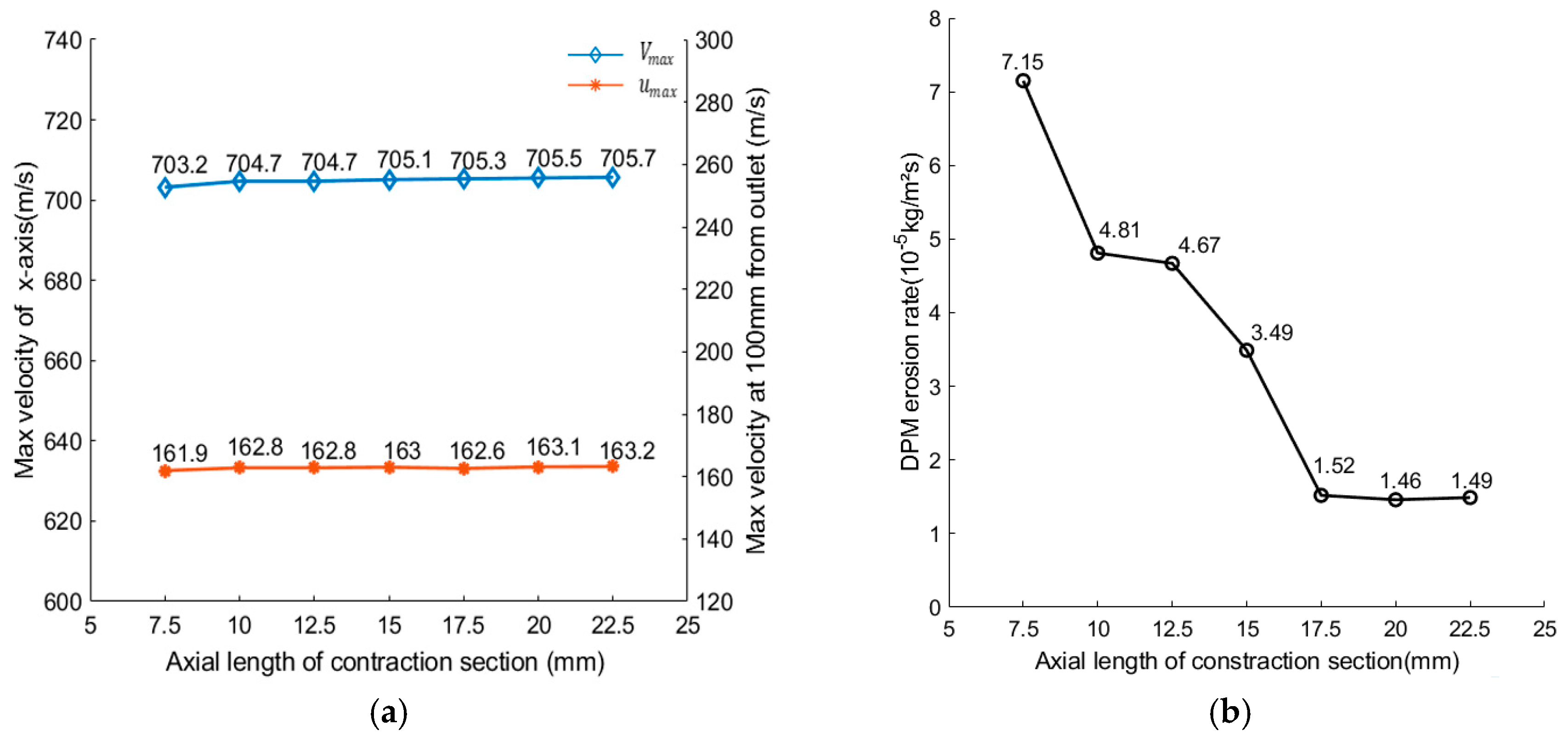
3.2.2. Effect of Axial Length of Contraction Section

It can be seen that with an increase in the axial length of the contraction section, $V_{max}$ only increased slightly, $u_{max}$ remained near constant and the $R_E$ value had a significant decrease, as shown in Figure 5a,b. Simulation results showed that the axial length of the contraction section mainly affected the life of the nozzle; the effect on the nozzle cutting capacity was limited.

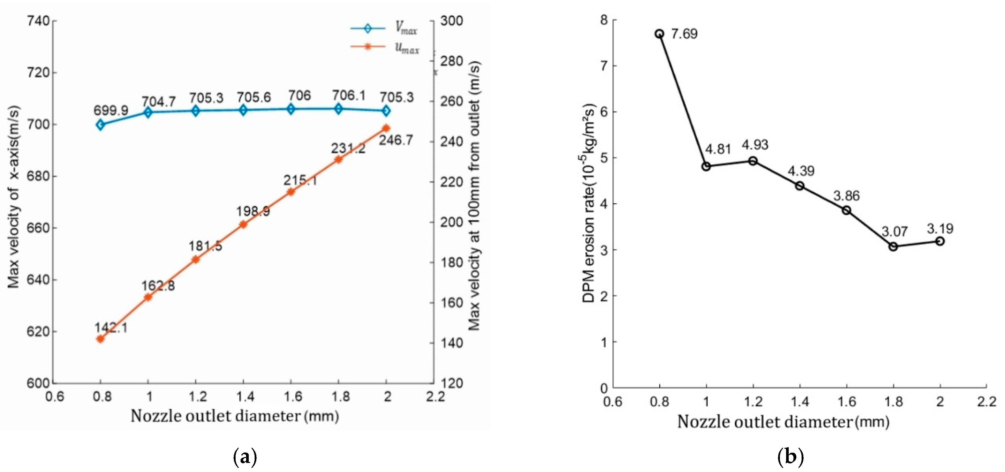
3.2.3. Effect of Outlet Diameter

Abrasive material in the focus section causes a violent, abrasive washout on the wall [27], which changes the shape of the nozzle so that the jet is not concentrated well. After increasing the nozzle diameter increased, the $V_{max}$ value increased slightly; the $u_{max}$ value increased rapidly, as shown in Figure 6a; and the $R_E$ value decreased first rapidly and then gently in Figure 6b. The rapid increase in the $u_{max} \mathrm{value}$ indicated that increasing outlet diameter can enhance nozzle cutting capacity, and the rapid decrease in the $R_E$ value indicated that increasing the nozzle-outlet diameter can extend nozzle life. It was also found that increasing the nozzle diameter led to an increase in the total flow rate of the water, as well as an increase in the total kinetic energy of the jet at both the outlet and the distance of 100 mm; thus, the cutting capacity of the nozzle was enhanced while the pressure was kept constant.

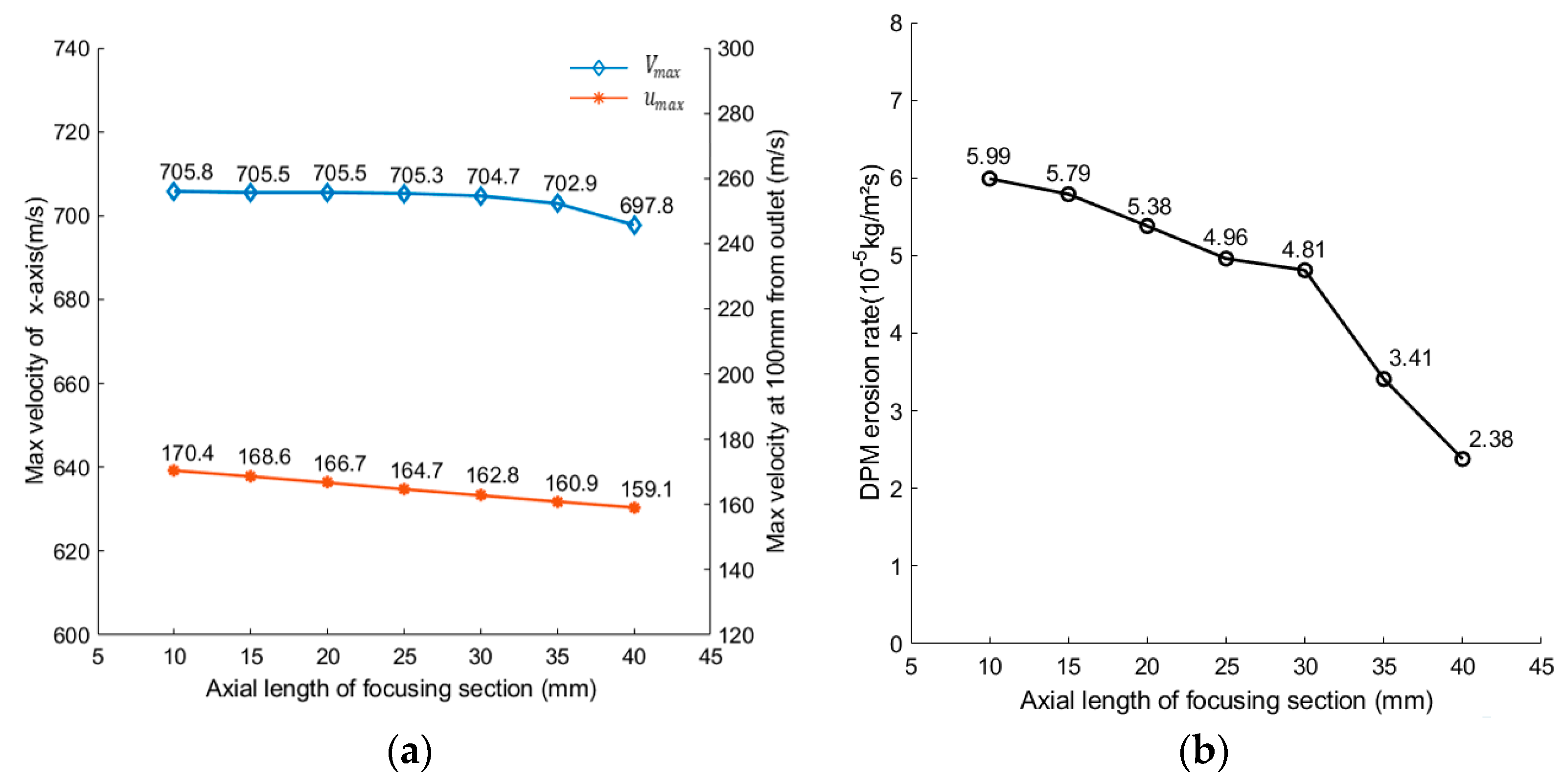
3.2.4. Effect of Axial Length of Focusing Section

$V_{max}$ and $u_{max}$ only decreased slightly and $R_E$ decreased rapidly when the axial length of the focus section increased, as shown in Figure 7a,b, indicating that focus-section length has a low effect on cutting ability but a high effect on nozzle service life. More energy was lost in longer focus sections, resulting in a decrease in the peak velocity of the jet. However, with the lower jet velocity, the flow rate of abrasive particles was also reduced, thus reducing the erosion on the inner wall of the nozzle.

The above analysis shows that the contraction curve and the axial length of the contraction section mainly affected the service life of the nozzle, and nozzle-outlet diameter mainly affected the cutting ability.

3.3. Nozzle Geometry Optimization

3.3.1. Orthogonal Experimental Design Method

Through the analysis above, the effects of nozzle parameters on nozzle performance are basically clear, but the optimal combination of nozzle parameters could not be obtained directly. If all parameter combinations were tested, the workload would be too big; the orthogonal experimental design can minimize the number of simulation tests to achieve results equivalent to those of full-scale tests [28,29], so the orthogonal experimental design was used to optimize the nozzle geometric parameters. There were four structural parameters of the nozzle, each of which had seven levels. According to the orthogonal design, the first four columns of the $L_{49} (7^8$) orthogonal table were selected for the simulation test. The factors and levels of the orthogonal tests are listed in

Table 4. Factors and levels.

Level (j)	$\mathit{A}$	$\mathit{B}$	$\mathit{C}$	$\mathit{D}$
	Contraction Curve	Axial Length of Contraction Section (mm)	Outlet Diameter (mm)	Axial Length of Focusing Section (mm)
1	$A_1$	7.5	0.8	10
2	$A_2$	10	1	15
3	$A_3$	12.5	1.2	20
4	$A_4$	15	1.4	25
5	$A_5$	17.5	1.6	30
6	$A_6$	20	1.8	35
7	$A_7$	22.5	2	40

.

The objective function, $Q$, is the nozzle performance excellence index with maximum velocity, $u_{max},$ and maximum erosion rate, $R_E$, as variables. The performance excellence index, $Q$, is defined as:

$${\mathrm{Q}}_i=0.5\frac{u_{max}^i}{u_{max}^0}+0.5EXP(-0.4\ast (\frac{R_E^i}{R_E^0}-1))$$

(9)

where $i$ indicates the ith test. The simulation results of the conical nozzle were used as a baseline, where $u_{max}^0=162.8 \mathrm{m}$/s and $R_E^0=4.81\times {10}^{-5} \mathrm{kg}/{\mathrm{m}}^2·\mathrm{s}$. The higher the $u_{max}^i$ value was, the better, and the lower the $R_E^i \mathrm{value}$ was, the better.

3.3.2. Simulation and Discussion

Based on the simulation results, the values of $Q$ were calculated and are listed in

Table 5. Table of orthogonal experiments and experimental data.

Factor	$\mathit{A}$	$\mathit{B}$	$\mathit{C}$	$\mathit{D}$	${\mathit{u}}_{\mathit{m}\mathit{a}\mathit{x}}^{\mathit{i}}$	${\mathit{R}}_{\mathit{E}}^{\mathit{i}}$	$\mathit{Q}$
Number (i)	1	2	3	4
1	$A_1$	7.5	0.8	10	147.7	1.78	1.097
2	$A_1$	10	1.2	25	182.7	2.91	1.147
3	$A_1$	12.5	1.6	40	211.5	3.63	1.201
4	$A_1$	15	2	20	248.7	2.85	1.352
5	$A_1$	17.5	1	35	158	1.28	1.156
6	$A_1$	20	1.4	15	202.1	1.49	1.280
7	$A_1$	22.5	1.8	30	229.3	1.99	1.336
8	$A_2$	7.5	2	35	245.6	5.91	1.211
9	$A_2$	10	1	15	168.7	2.05	1.147
10	$A_2$	12.5	1.4	30	198.3	3.45	1.169
11	$A_2$	15	1.8	10	237.3	2.35	1.342
12	$A_2$	17.5	0.8	25	141.9	0.87	1.130
13	$A_2$	20	1.2	40	177.5	1.57	1.200
14	$A_2$	22.5	1.6	20	222.6	2.37	1.296
15	$A_3$	7.5	1.8	25	233.2	5.84	1.175
16	$A_3$	10	0.8	40	135.4	1.92	1.052
17	$A_3$	12.5	1.2	20	190.9	1.84	1.226
18	$A_3$	15	1.6	35	214.1	1.87	1.296
19	$A_3$	17.5	2	15	236	1.82	1.366
20	$A_3$	20	1	30	162.9	0.61	1.209
21	$A_3$	22.5	1.4	10	205.7	0.93	1.322
22	$A_4$	7.5	1.6	15	220.6	3.02	1.258
23	$A_4$	10	2	30	246.8	2.84	1.347
24	$A_4$	12.5	1	10	169.9	0.82	1.219
25	$A_4$	15	1.4	25	200.3	0.96	1.304
26	$A_4$	17.5	1.8	40	227.8	1.71	1.347
27	$A_4$	20	0.8	20	144.1	0.33	1.168
28	$A_4$	22.5	1.2	35	179.1	0.38	1.273
29	$A_5$	7.5	1.4	40	194.8	6.99	1.015
30	$A_5$	10	1.8	20	234.1	3.29	1.286
31	$A_5$	12.5	0.8	35	138.5	4.89	0.922
32	$A_5$	15	1.2	15	187.2	1.92	1.211
33	$A_5$	17.5	1.6	30	215.6	1.32	1.331
34	$A_5$	20	2	10	253	1.42	1.439
35	$A_5$	22.5	1	25	164.9	1.47	1.167
36	$A_6$	7.5	1.2	30	181.5	3.93	1.095
37	$A_6$	10	1.6	10	221.7	2.44	1.290
38	$A_6$	12.5	2	25	247.8	3.42	1.322
39	$A_6$	15	1	40	158	1.11	1.165
40	$A_6$	17.5	1.4	20	201.1	2.54	1.222
41	$A_6$	20	1.8	35	228.5	2.13	1.327
42	$A_6$	22.5	0.8	15	145.9	0.67	1.154
43	$A_7$	7.5	1	20	166.7	1.89	1.149
44	$A_7$	10	1.4	35	197.1	3.13	1.180
45	$A_7$	12.5	1.8	15	235.5	3.55	1.279
46	$A_7$	15	0.8	30	138.8	0.71	1.129
47	$A_7$	17.5	1.2	10	186.9	1.38	1.239
48	$A_7$	20	1.6	25	215.8	1.57	1.317
49	$A_7$	22.5	2	40	243.1	1.74	1.392

beside the orthogonal design parameters.

A statistical analysis and an ANOVA were performed based on the values of $Q$ in Table 5, and the results thereof are presented in

Table 6. Statistical analysis.

Level (j)	$\mathit{A}$	$\mathit{B}$	$\mathit{C}$	$\mathit{D}$
$k_1$	1.224	1.143	1.093	1.278
$k_2$	1.213	1.207	1.173	1.242
$k_3$	1.235	1.191	1.199	1.243
$k_4$	1.274	1.257	1.213	1.223
$k_5$	1.195	1.256	1.284	1.231
$k_6$	1.225	1.278	1.299	1.195
$k_7$	1.241	1.277	1.347	1.196
$RG$	0.060	0.134	0.244	0.083
Superior level	4	6	7	1
Factor priority	4	2	1	3

and

Table 7. Analysis of variance table.

Source of Variance	Deviation Sum of Squares	Degree of Freedom	Variance	$\mathit{F}$	Significant Level
$A$	0.025	6	0.004	3.153	*
$B$	0.108	6	0.018	13.869	***
$C$	0.313	6	0.052	40.018	****
$D$	0.036	6	0.006	4.574	**
Error	0.031	24	0.001
Sum		48

$F_{0.05}\left(6,24\right)=$2.51; * indicates the level of significance, the higher the number the more significant.

.

In the statistical analysis, $RG$ stands for the variation range, which is used to compare importance of different factors to the optimization objective and can be calculated using Equation (10). The higher the RG value is, the more important the factor is, as shown by

$$RG=\max \left(k_j\right)-\min \left(k_j\right)$$

(10)

where $k_j$ represents the average of the results to which the $j$th level of each factor leads. A higher $k_j$ value indicates a better level.

The superior levels are the level with the maximum $k_j$ (j = 1 to 7) for each factor, as listed in Table 6; this was (4,6,7,1) for factors ($A,B,C,D$). Correspondingly, the optimal parameter combination was ($A$ = $A_4$, $B$ = $B_6$ = 20 mm, $\mathrm{C}$ = $C_7$ = 2 mm, $\mathrm{D}$ = $D_1$ = 10 mm).

Factor priority can be identified according to the RG value of each factor. According to Table 6, the priority sequence is $C$ > $B$ >$D$ > $A$.

Analysis of variance (ANOVA) can also help to identify factor priority or significance, as listed in Table 7.

The $F$-test is used for ANOVA with a significant level of 0.05, and according to the table of critical values for the $F$-test, the critical value is $F_{0.05}\left(6,24\right)=2$.51. Meanwhile, the larger the $F$ value is, the more significant the factor is. Analysis results show that all factors, $A, B,C$ and $D,$ had an effect on the performance excellence index, $Q$; factor $C$ had the greatest impact on the nozzle performance, and after that were $B, D$ and $A$. The results of the ANOVA and the statistical analysis agree with each other very well.

The optimal combination was not in the 49 sets of experiments, as listed in Table 5, so the optimal nozzle was simulated separately, as shown in Figure 8; $u_{max}=252.2 \mathrm{m}/\mathrm{s}$, $R_E=$ $1.35\times {10}^{-5} \mathrm{kg}/{\mathrm{m}}^2·\mathrm{s}$ and nozzle performance excellence index $Q$ = 1.441, which was the best result in all simulation tests, consistently with the theoretical analysis. The performance of this nozzle was 44.4% higher than that of the conical nozzle, the maximum velocity at the distance of 100 mm was 56% higher and the maximum erosion rate of the nozzle was 72% lower.

4. Conclusions

This paper proposes an orthogonal experimental design based optimization method for the nozzle geometry of an underwater abrasive water jet with the objective of maximizing the cutting capacity and minimizing the nozzle-erosion rate. Four factors (parameters), with seven levels each, were involved in this optimization, including the contraction-section curve, the contraction-section axial length, the nozzle-outlet diameter and the focus section length.

The parameter effects on the nozzle cutting capability and life were analyzed.

The following conclusions can be drawn.

(1)

The contraction section curve, axial length of contraction section and axial length of focusing section mainly affect the nozzle service life, while nozzle-outlet diameter mainly affects nozzle cutting capacity.

(2)

The effect significances of the structural parameters, from high to low, are: outlet diameter > axial length of contraction section > axial length of focusing section > contraction curve.

(3)

According to the optimal performance index of the nozzle, the optimal nozzle structure parameters are a contraction curve of $A_4$ (parabolic), an axial length of contraction section of 20 mm, an outlet diameter of 2 mm, and an axial length of focusing section of 10 mm.

(4)

With the optimal parameters, the nozzle performance excellence index is $Q$ = 1.441, which is the optimization objective and 44.1% higher than the baseline of the conical nozzle; the maximum velocity at a distance of 100 mm is improved by 56% and the maximum erosion rate is reduced by 72% compared to those of the conical nozzle.

In future work, the cutting capacity of the optimal nozzle and the effects of operating parameters on cutting capacity and nozzle life need to be experimentally verified.

References

1. Llanto, J.M.; Tolouei-Rad, M.; Aamir, M. Recent Progress Trend on Abrasive Waterjet Cutting of Metallic Materials: A Review. Appl. Sci. 2021, 11, 3344. [Google Scholar] [CrossRef]
2. Liu, X.C.; Liang, Z.W.; Wen, G.L.; Yuan, X.F. Waterjet machining and research developments: A review. Int. J. Adv. Manuf. Technol. 2019, 102, 1257–1335. [Google Scholar] [CrossRef]
3. Haldar, B.; Ghara, T.; Ansari, R.; Das, S.; Saha, P. Abrasive jet system and its various applications in abrasive jet machining, erosion testing, shot-peening, and fast cleaning. Mater. Today Proc. 2018, 5 Pt 2, 13061–13068. [Google Scholar] [CrossRef]
4. Cao, L.P.; Liu, S.; Huang, Y.S.; Liu, Q.; Li, Z.H. Study of high-pressure waterjet characteristics based on CFD simulation. Appl. Mech. Mater. 2012, 224, 307–311. [Google Scholar] [CrossRef]
5. Yu, Y.; Sun, T.X.; Gao, H.; Wang, X.P. Experimental investigation into the effect of abrasive process parameters on the cutting performance for abrasive waterjet technology: A case study. Int. J. Adv. Manuf. Technol. 2020, 107, 2757–2765. [Google Scholar] [CrossRef]
6. Khan, A.A.; Munajat, N.B.; Tajudin, H.B. A Study on Abrasive Water Jet Machining of Aluminum with Garnet Abrasives. J. Appl. Sci. 2005, 5, 1650–1654. [Google Scholar] [CrossRef]
7. Liao, W.T.; Deng, X.Y. Study on Flow Field Characteristics of Nozzle Water Jet in Hydraulic cutting. IOP Conf. Ser. Earth Environ. Sci. 2017, 81, 012167. [Google Scholar] [CrossRef] [Green Version]
8. Khan, A.A.; Haque, M.M. Performance of different abrasive materials during abrasive water jet machining of glass. J. Mater. Process. Technol. 2007, 191, 404–407. [Google Scholar] [CrossRef]
9. Chen, X.C.; Deng, S.S.; Hua, W.X. Experiment and simulation research on abrasive water jet nozzle wear behavior and anti-wear structural improvement. J. Braz. Soc. Mech. Sci. Eng. 2017, 39, 2023–2033. [Google Scholar] [CrossRef]
10. Pi, V.N.; Tuan, N.Q. A study on nozzle wear modeling in Abrasive Waterjet Cutting. Adv. Mater. Res. 2009, 78, 345–350. [Google Scholar] [CrossRef]
11. Du, M.M.; Wang, H.J.; Guo, Y.J.; Ke, Y.L. Numerical research on multi-particle movements and nozzle wear involved in abrasive waterjet machining. Int. J. Adv. Manuf. Technol. 2021, 117, 2845–2858. [Google Scholar] [CrossRef]
12. Ding, M.W.; Fu, C.J.; Yin, S.B. Optimization on the Structure of Ceramic Nozzles by FLUENT Simulation. Appl. Mech. Mater. 2013, 397–400, 213–217. [Google Scholar] [CrossRef]
13. Liu, Y.L.; Zhu, H.Q.; Huang, S.G. Effect of structural parameters of high-pressure water jet nozzles on flow field features. Int. J. Heat Technol. 2017, 4, 707–712. [Google Scholar] [CrossRef]
14. Deepak, D.; Jodel, A.Q.; Midhun, A.M.; Shiva, P.U. Numerical analysis of the effect of nozzle geometry on flow parameters in abrasive water jet machines. Sci. Technol 2017, 2, 497–506. [Google Scholar]
15. Wen, J.W.; Qi, Z.W.; Behbahani, S.S.; Pei, X.J.; Iseley, T. Research on the structures and hydraulic performances of the typical direct jet nozzles for water jet technology. J. Braz. Soc. Mech. Sci. Eng. 2019, 41, 570. [Google Scholar] [CrossRef]
16. Zhang, Y.X.; Wang, L.F.; Yao, F.; Wang, H.; Men, X.H.; Ye, B.B. Experimental Study on the Influence of Nozzle Diameter on abrasive jet Cutting Performance. Adv. Mater. Res. 2011, 337, 466–469. [Google Scholar] [CrossRef]
17. Nanduri, M.; Taggart, D.G.; Kim, T.J. The effects of system and geometric parameters on abrasive water jet nozzle wear. Int. J. Mach. Tools Manuf. 2002, 42, 615–623. [Google Scholar] [CrossRef]
18. Guan, J.F.; Deng, S.S.; Jiao, G.W.; Chen, M.; Hua, W.X. Numerical Simulation Study of Influence of Nozzle Entrance Diameter on Jet Performance of Pre-mixed Abrasive Water Jet. Appl. Mech. Mechatron. Intell. Syst. 2015, 2016, 57–62. [Google Scholar]
19. Syazwani, H.; Mebrahitom, G.; Azmir, A. A review on nozzle wear in abrasive water jet machining application. IOP Conf. Ser. Mater. Sci. Eng. 2016, 114, 12020–12027. [Google Scholar] [CrossRef]
20. Liu, H.; Wang, J.; Kelson, N.; Brown, R.J. A study of abrasive waterjet characteristics by CFD simulation. J. Mater. Process. Technol. 2004, 153–154, 488–493. [Google Scholar] [CrossRef] [Green Version]
21. Long, X.P.; Ruan, X.P.; Liu, Q.; Xue, S.X.; Wu, Z.Q. Numerical investigation on the internal flow and the particle movement in the abrasive waterjet nozzle. Powder Technol. 2017, 314, 635–640. [Google Scholar] [CrossRef]
22. Toapanta-Ramos, L.F.; Zapata-Cautillo, J.A.; Cholango-Gvailanes, A.I.; Qutiaquez, W.; Nieto-Londono, C.; Zapata-Benabithe, Z. Numerical and comparative study of the turbulence effect on elbows and bends for sanitary water distribution. Rev. Fac. De Ing. 2019, 28, 101–118. [Google Scholar] [CrossRef]
23. Kamarudin, N.H.; Prasada Rao, A.K.; Azhari, A. CFD Based Erosion Modelling of Abrasive Waterjet Nozzle using Discrete Phase Method. IOP Conf. Ser. Mater. Sci. Eng. 2016, 114, 12016–12023. [Google Scholar] [CrossRef] [Green Version]
24. Pătîrnac, I.; Ripeanu, R.; Laudacescu, G.E. Abrasive flow modelling through active parts water jet machine using CFD simulation. IOP Conf. Ser. Mater. Sci. Eng. 2020, 724, 12001–12006. [Google Scholar] [CrossRef]
25. Soyama, H. Effect of nozzle geometry on a standard cavitation erosion test using a cavitating jet. Wear 2013, 297, 895–902. [Google Scholar] [CrossRef]
26. Chen, J.; Guo, L.W.; Hu, Y.W.; Chen, Y. Internal structure of a jet nozzle for coalbed methane mining based on airfoil curves. Shock Vib. 2018, 2018, 3840834. [Google Scholar] [CrossRef]
27. Deepak, D.; Anjaiah, D.; Vasudeve, K.K.; Sharma, N.Y. CFD simulation of flow in an abrasive water suspension jet: The effect of inlet operating pressure and volume fraction on skin friction and exit kinetic energy. Adv. Mech. Eng. 2011, 2192, 2004–2008. [Google Scholar] [CrossRef]
28. Li, S.L.; Wu, G.G.; Wang, P.F.; Cui, Y.; Tian, C.; Han, H. A mathematical model for predicting the sauter mean diameter of Liquid-Medium ultrasonic atomizing nozzle based on orthogonal design. Appl. Sci. 2021, 11, 11628. [Google Scholar] [CrossRef]
29. Shen, C.M.; Lin, B.Q.; Meng, F.W. Structure optimization and application of conical convergence high-pressure jet nozzle. Adv. Mater. Res. 2011, 228–229, 1001–1006. [Google Scholar] [CrossRef]
Figure 1. Nozzle-shape cross-section.
Machines 10 01243 g001
Figure 2. CFD simulation model.
Machines 10 01243 g002
Figure 3. Shapes of contraction curves.
Machines 10 01243 g003
Figure 4. Effect of contraction curves on the performance of the nozzle: (a) Effect of contraction curve on jet velocity; (b) Effect of contraction curve on R E .
Machines 10 01243 g004
Figure 5. Effect of axial length of contraction section: (a) Effect of the axial length of contraction section on jet velocity; (b) Effect of the axial length of contraction section on R E .
Machines 10 01243 g005
Figure 6. Effect of outlet diameter: (a) Effect of outlet diameter on jet velocity; (b) Effect of outlet diameter on R E .
Machines 10 01243 g006
Figure 7. Effect of the axial length of the focusing section: (a) Effect of he axial length of the focusing section on jet velocity; (b) Effect of he axial length of the focusing section on R E .
Machines 10 01243 g007
Figure 8. Velocity distribution of the optimal nozzle.
Machines 10 01243 g008