
Nonlinear Analysis of Rotor-Bearing-Seal System with Varying Parameters Muszynska Model Based on CFD and RBF


Abstract
:1. Introduction
2. The Muszynska Nonlinear Seal Force Model
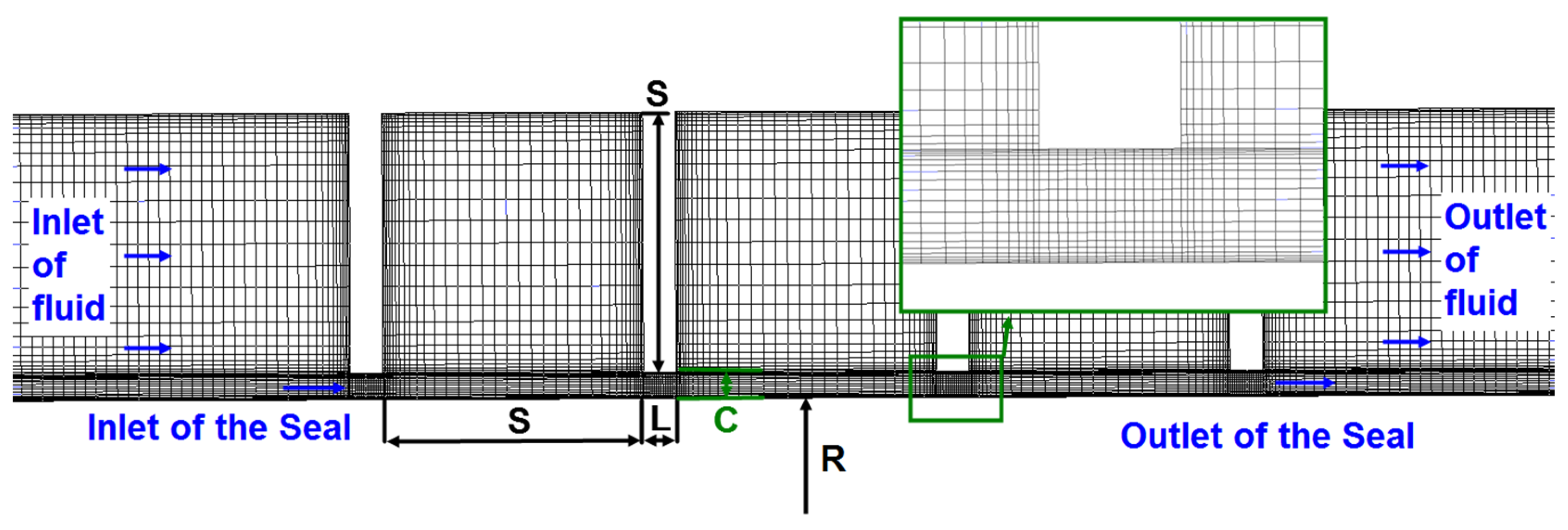
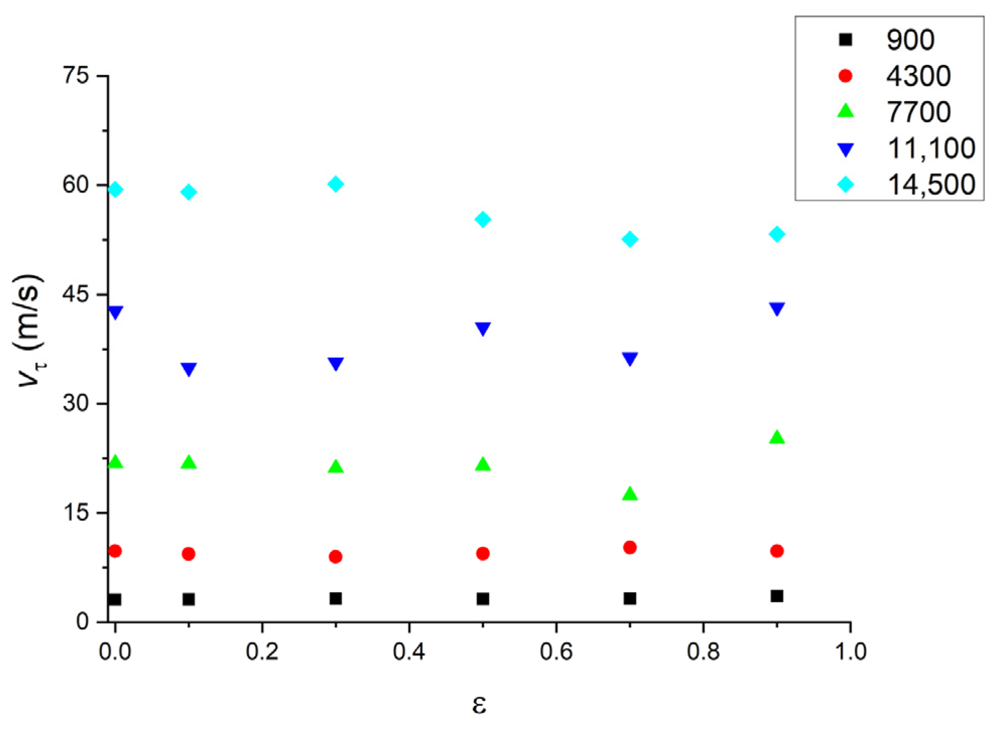
3. CFD Simulation
4. The Response Surface by RBF
5. Rotor Dynamics Analysis of Varying Parameters
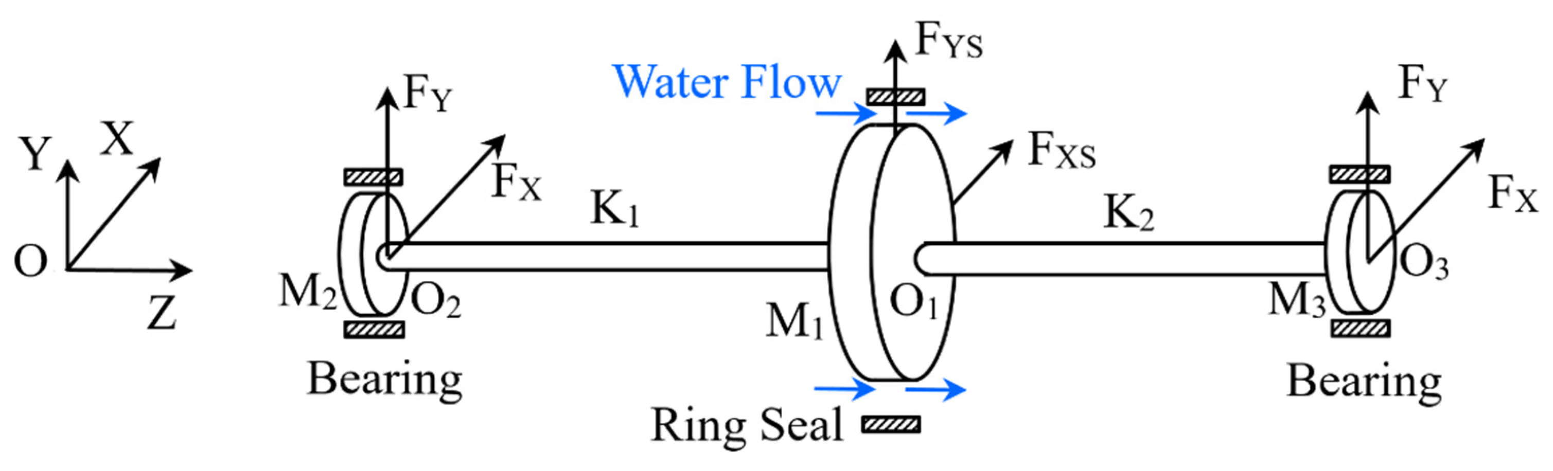
5.1. Numerical Model and Governing Equations
5.2. Comparing the Rotor Dynamic Characteristics of the VP Method to the Traditional method
- (1)
- When rad/s, the amplitude of the rotor increases gradually. Following this, with the increase in rotational speed, the amplitude of the rotor decreases gradually. It can be identified that ωn = 300 rad/s is the first-order critical speed of the rotor system;
- (2)
- When rad/s, the bifurcation has been observed and the amplitude value increases;
- (3)
- When rad/s, the amplitude of the bearing increases again substantially, with the maximum close to value 1.
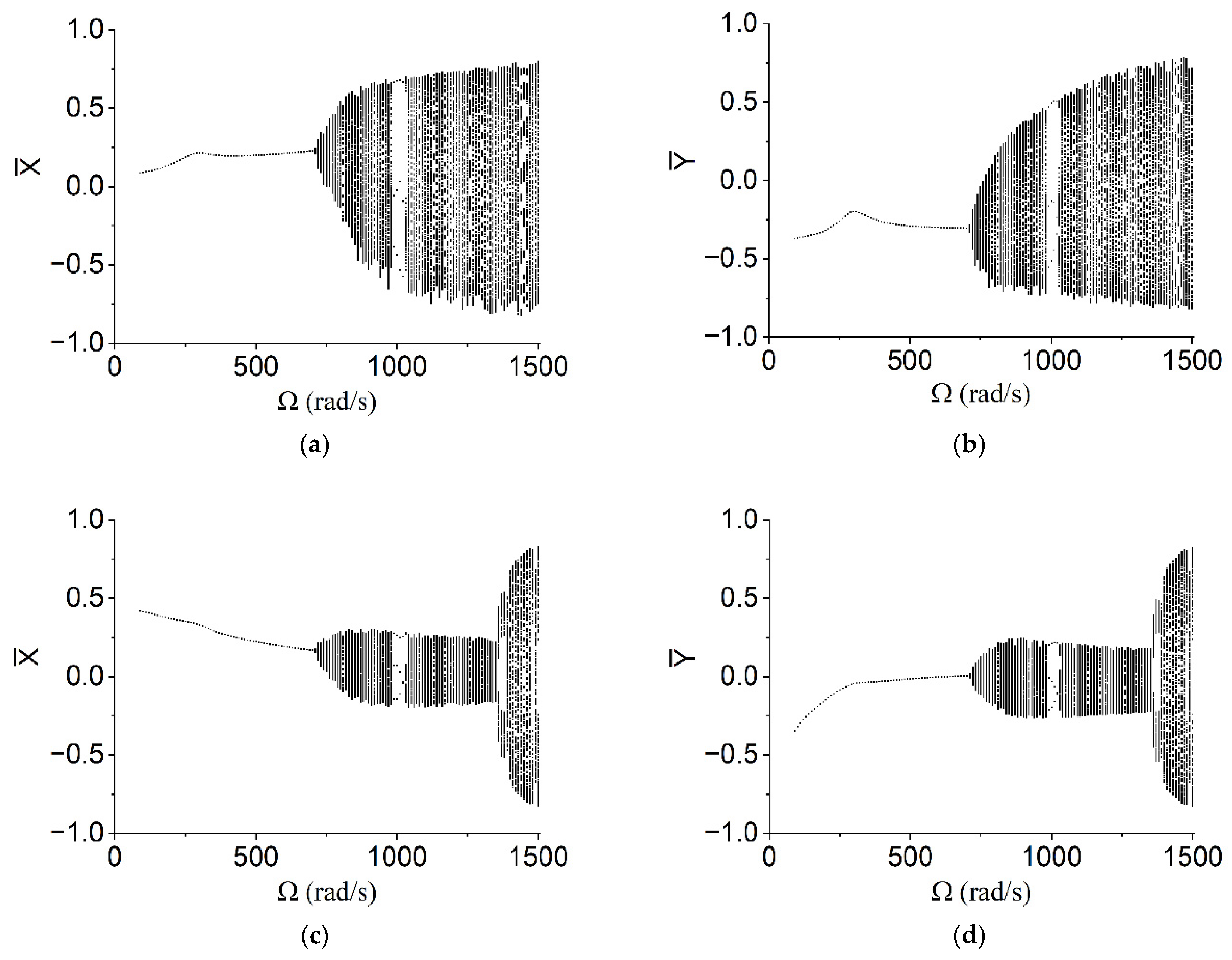
- (1)
- When rad/s, the conclusion is same as item (1) in Figure 10. It can be identified that ωn = 300 rad/s is the first-order critical speed of the rotor system;
- (2)
- When rad/s, the bifurcation is observed and the amplitude value increases;
- (3)
- When rad/s, the amplitude of the bearing increases again substantially, with the maximum close to value 1.
- (1)
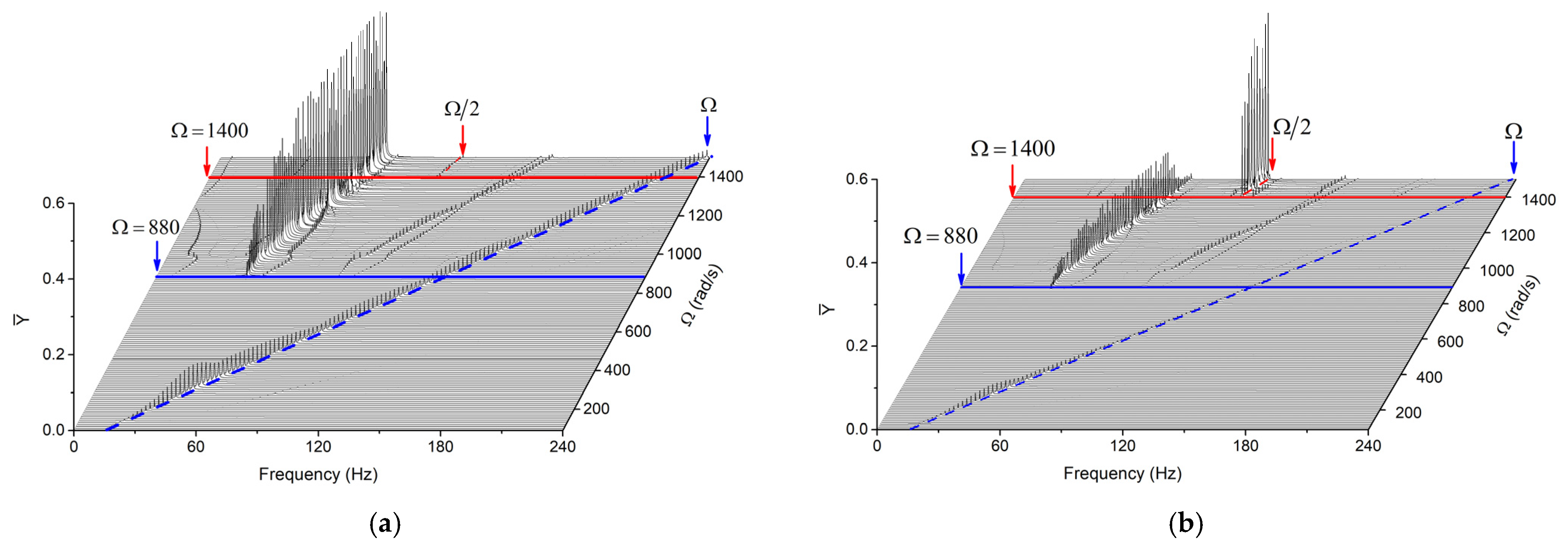
- When rad/s, there is only the frequency component corresponding to the rotational speed (Ω) at the rotor and bearing;
- (2)
- When rad/s, there are many frequency components at the rotor and bearing. When rad/s, a half-frequency (Ω/2) component of rotational speed appears at the rotor and bearing. In addition, the half-frequency component of the speed at the bearing is significantly higher than the peaks of the others that dominate. According to the literature [25], it can be judged that the oil film whirl occurred at the bearing, and Ω = 1400 rad/s is the oil film instability velocity of the rotor system.
- (1)
- When rad/s, there is only the frequency component corresponding to the rotational speed (Ω) at the rotor and bearing;
- (2)
- When rad/s, there are several frequency components at the rotor and bearing. It is worth noting that when rad/s, the half-frequency (Ω/2) of the rotational speed appears at the rotor and bearing. Furthermore, the half-frequency component at the bearing is obviously higher than the peaks of the other frequency components that are dominant. According to the literature [25,26], it can be judged that the oil film whirl occurred at the bearing. Thus, Ω = 1360 rad/s is the oil film instability angular velocity of the rotor system.
5.3. Axis Trajectories, Phase Diagrams and Poincaré Diagrams of the VP Method in Several Characteristic Speeds
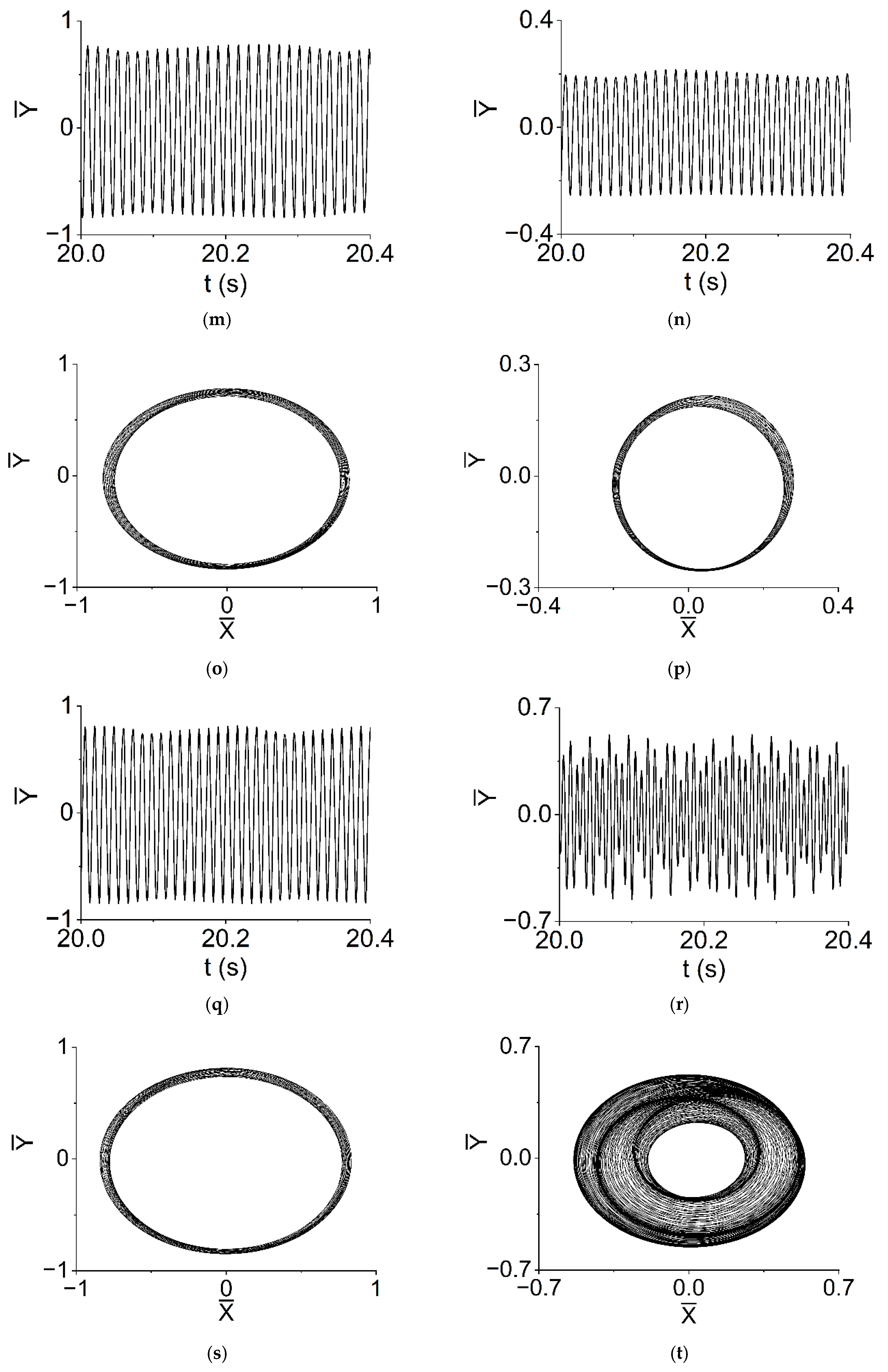
- (1)
- When rad/s, the periodic motion can be observed at rotor and bearings. The displacements of rotor and bearings are periodic; the shape of the trajectories and phases of rotor and bearings are a closed circle, respectively; there is only one point on each Poincaré map;
- (2)
- When and rad/s, the quasi-periodic motion can be obtained. The envelopes of displacements of rotor and bearings are periodic; the shapes of the trajectories and phases of rotor and bearings are quasi-periodic, respectively; most of the points on each Poincaré map formed a ring shape, while the shape in Figure 16h resembles a number eight;
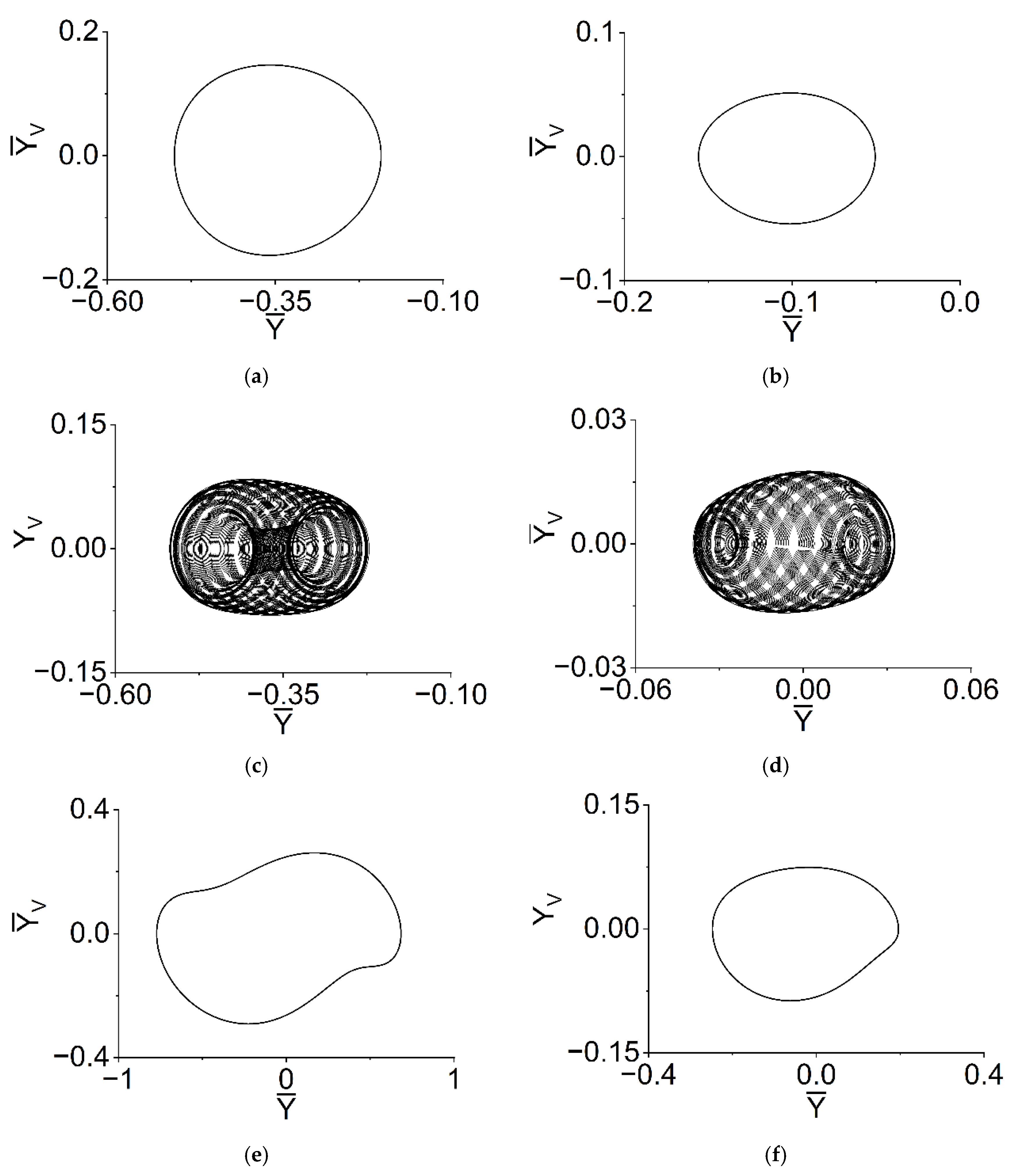
- (3)
- When rad/s, both the rotor and the bearing have a three-fold period bifurcation. The displacements of rotor and bearings are periodic; the shape of the trajectories and phases of rotor and bearings are a closed circle, respectively; there are three isolated points on the Poincaré map (Ω = 1250 rad/s, as Figure 16e,f), which correspond to 1/3 harmonic of the system;
- (4)
- When rad/s, the envelopes of displacements of rotor and bearings are periodic; the shape of the trajectories and phases of rotor and bearings are quasi-periodic, respectively; the rupture of phase trajectory in the bearing can be observed, as in Figure 16j.
6. Conclusions
- (1)
- The results of the first-order critical speed of the system are obtained by way of both the traditional constant model and the varying parameters model based on the approximate function surface method and the CFD method. The result obtained by the two methods is the same, which is equal to 300 rad/s;
- (2)
- In the process of increasing the speed, the results of both models appeared to have quasi-periodic motion. The difference is that the speed corresponding to the bifurcation point based on the traditional constant model is lower than that of the varying parameters model;
- (3)
- The oil film whirl phenomenon of the rotor-bearing-seal system is obtained by both algorithms. The difference is that the oil film instability angular velocity obtained based on the traditional constant model is lower than that of the varying parameters model. This means that the rotor-bearing-seal system in fact has a larger stable operation range.
Author Contributions
Funding
Data Availability Statement
Conflicts of Interest
References
- Black, H.F. Effects of Hydraulic Forces in Annular Pressure Seals on the Vibrations of Centrifugal Pump Rotors. J. Mech. Eng. Sci. 1969, 11, 206–213. [Google Scholar] [CrossRef]
- Childs, D.W. Dynamic Analysis of Turbulent Annular Seals Based on Hirs’ Lubrication Equation. J. Lubr. Technol. 1983, 105, 429–436. [Google Scholar] [CrossRef]
- Childs, D.W. Finite-Length Solutions for Rotordynamic Coefficients of Turbulent Annular Seals. J. Lubr. Technol. 1983, 105, 437–445. [Google Scholar] [CrossRef]
- Childs, D.W.; Scharrer, J.K. An Iwatsubo-Based Solution for Labyrinth Seals Comparison to Experimental Results. J. Eng. Gas Turbines Power-Trans. ASME 1986, 108, 325–331. [Google Scholar] [CrossRef] [Green Version]
- Childs, D.W.; Wade, J. Rotordynamic-Coefficient and Leakage Characteristics for Hole-Pattern-Stator Annular Gas Seals-Measurements versus Predictions. J. Tribol.-Trans. ASME 2004, 126, 326–333. [Google Scholar] [CrossRef]
- Childs, D.W.; McLean, J.; Zhang, M.; Arthur, S. Rotordynamic Performance of a Negative-Swirl Brake for a Tooth-on-Stator Labyrinth Seal. J. Eng. Gas Turbines Power ASME 2016, 138, 062505. [Google Scholar] [CrossRef]
- Nelson, C.C. Comparison of Hirs’ Equation with Moody’s Equation for Determining Rotordynamic Coefficients of Annular Pressure Seals. J. Tribol.-Trans. ASME 1987, 109, 144–148. [Google Scholar] [CrossRef] [Green Version]
- Muszynska, A. Whirl and Whip–Rotor Bearing Stability Problems. J. Sound Vib. 1986, 110, 443–462. [Google Scholar] [CrossRef] [Green Version]
- Bently, D.E.; Muszynska, A. Role of Circumferential Flow in the Stability of Fluid Handling Machine Rotors; Bently Rotor Dynamics Research Corporation: Minden, NV, USA, 1989; pp. 415–430. [Google Scholar]
- Muszynska, A.; Bently, D.E.; Franklin, W.D.; Grant, J.W.; Goldman, P. Applications of Sweep Frequency Rotating Force Perturbation Methodology in Rotating Machinery for Dynamic Stiffness Identification. J. Eng. Gas Turbines Power-Trans. ASME 1993, 115, 266–271. [Google Scholar] [CrossRef]
- Li, S.T.; Xu, Q.Y.; Zhang, X.L. Nonlinear Dynamic Behaviors of a Rotor-Labyrinth Seal System. Nonlinear Dyn. 2007, 47, 321–329. [Google Scholar] [CrossRef]
- Wang, Y.F.; Wang, X.Y. Nonlinear Vibration Analysis for a Jeffcott Rotor with Seal and Air-Film Bearing Excitations. Math. Probl. Eng. 2010, 2010, 657361. [Google Scholar] [CrossRef] [Green Version]
- Zhang, E.Z.; Jiao, Y.H.; Chen, Z.B. Dynamic behavior analysis of a rotor system based on a nonlinear labyrinth-seal forces model. J. Comput. Nonlinear Dyn. 2018, 13, 101002. [Google Scholar] [CrossRef]
- Xu, Q.; Luo, Y.; Yao, H.; Zhao, L.; Wen, B. Eliminating the Fluid-Induced Vibration and Improving the Stability of the Rotor/Seal System Using the Inerter-Based Dynamic Vibration Absorber. Shock. Vib. 2019, 2019, 1–9. [Google Scholar] [CrossRef]
- Zhang, K.; Jiang, X.; Li, S.; Huang, B.; Yang, S.; Wu, P.; Wu, D. Transient CFD Simulation on Dynamic Characteristics of Annular Seal under Large Eccentricities and Disturbances. Energies 2020, 13, 4056. [Google Scholar] [CrossRef]
- Mutra, R.R.; Srinivas, J. Parametric design of turbocharger rotor system under exhaust emission loads via surrogate model. J. Braz. Soc. Mech. Sci. Eng. 2021, 43, 1–17. [Google Scholar] [CrossRef]
- Moore, J.J. Three-Dimensional CFD Rotordynamic Analysis of Gas Labyrinth Seals. J. Vib. Acoust. 2003, 125, 427–433. [Google Scholar] [CrossRef]
- Li, Z.; Chen, Y.; Chen, Z.; Jiao, Y.; Ma, W. Nonlinear Dynamic Characteristics Analysis of the Gas Exciting Force in the Rotor-Seal System. J. Dyn. Control 2013, 11, 126–132. (In Chinese) [Google Scholar]
- Luo, Y.; Wang, P.; Jia, H.; Huang, F. Dynamic Characteristics Analysis of a Seal-Rotor System with Rub-Impact Fault. J. Comput. Nonlinear Dyn. 2021, 16, 081003. [Google Scholar] [CrossRef]
- Menter, F.R. Two-equation eddy-viscosity turbulence models for engineering applications. Aiaa J. 1994, 32, 1598–1605. [Google Scholar] [CrossRef] [Green Version]
- Hirano, T.; Guo, Z.L.; Kirk, R.G. Application of Computational Fluid Dynamics Analysis for Rotating Machinery—Part II Labyrinth Seal Analysis. J. Eng. Gas Turbines Power-Trans. ASME 2005, 127, 820–826. [Google Scholar] [CrossRef]
- Wang, Z.H.; Xu, L.Q.; Xi, G. Numerical Investigation on the Labyrinth Seal Design for a Low Flow Coefficient Centrifugal Compressor. In Proceedings of the ASME Turbo Expo 2010: Power for Land, Sea, and Air. Volume 7: Turbomachinery, Parts A, B, and C, Glasgow, UK, 14–18 June 2010; ASME; pp. 2031–2041. [Google Scholar]
- Zhang, H.X.; Huang, W.Q.; Wang, Y.; Lu, L.; Lyu, S. Research on Meshfree Method for Analyzing Seal Behavior of a T-DGS. Int. J. Precis. Eng. Manuf. 2017, 18, 529–536. [Google Scholar] [CrossRef]
- Wang, R.; Guo, X.L.; Wang, Y.F. Nonlinear analysis of rotor system supported by oil lubricated bearings subjected to base movements. Proc. Inst. Mech. Eng. Part C J. Mech. Eng. Sci. 2016, 230, 543–558. [Google Scholar] [CrossRef]
- Muszynska, A. Stability of Whirl and Whip in Rotor/Bearing Systems. J. Sound Vib. 1988, 127, 49–64. [Google Scholar] [CrossRef]
- Cheng, M.; Meng, G.; Jing, J.P. Non-linear dynamics of a rotor-bearing-seal system. Arch. Appl. Mech. 2006, 76, 215–227. [Google Scholar] [CrossRef]


| Inlet | Outlet | |
|---|---|---|
| Pressure | Axial Velocity | Pressure |
| 0.9 MPa | 10 m/s | 0.4 MPa |
| The First-Order Critical Speed | Bifurcation Point | Oil Film Instability Angular Velocity | |
|---|---|---|---|
| VP method | 300 | 880 | 1400 |
| Traditional constant method | 300 | 710 | 1360 |
Publisher’s Note: MDPI stays neutral with regard to jurisdictional claims in published maps and institutional affiliations. |
© 2022 by the authors. Licensee MDPI, Basel, Switzerland. This article is an open access article distributed under the terms and conditions of the Creative Commons Attribution (CC BY) license (https://creativecommons.org/licenses/by/4.0/).
Share and Cite
Wang, R.; Wang, Y.; Cao, X.; Yang, S.; Guo, X. Nonlinear Analysis of Rotor-Bearing-Seal System with Varying Parameters Muszynska Model Based on CFD and RBF. Machines 2022, 10, 1238. https://doi.org/10.3390/machines10121238
Wang R, Wang Y, Cao X, Yang S, Guo X. Nonlinear Analysis of Rotor-Bearing-Seal System with Varying Parameters Muszynska Model Based on CFD and RBF. Machines. 2022; 10(12):1238. https://doi.org/10.3390/machines10121238
Chicago/Turabian StyleWang, Rui, Yuefang Wang, Xiaojian Cao, Shuhua Yang, and Xinglin Guo. 2022. "Nonlinear Analysis of Rotor-Bearing-Seal System with Varying Parameters Muszynska Model Based on CFD and RBF" Machines 10, no. 12: 1238. https://doi.org/10.3390/machines10121238