Article

Real-Time Prediction of Remaining Useful Life for Composite Laminates with Unknown Inputs and Varying Threshold

1
School of Aeronautic Science and Engineering, Beihang University, Beijing 100191, China
2
Aircraft and Propulsion Laboratory, Ningbo Institute of Technology, Beihang University, Ningbo 315100, China
3
School of Reliability and Systems Engineering, Beihang University, Beijing 100191, China
*
Author to whom correspondence should be addressed.
Machines 2022, 10(12), 1185; https://doi.org/10.3390/machines10121185
Submission received: 8 November 2022 / Revised: 29 November 2022 / Accepted: 5 December 2022 / Published: 7 December 2022
(This article belongs to the Section Material Processing Technology)

Abstract

:
Prognostics and health management (PHM) has emerged as an essential approach for improving the safety, reliability, and maintainability of composite structures. However, an obstacle remains in its damage state estimation and lifetime prediction due to unknown inputs. Thus, a self-calibration Kalman-filter-based framework for residual life prediction is proposed, which involves unknown input items in the fatigue damage evolution model and employs health-monitoring data to estimate and compensate for them. Combined with the time-varying structural failure threshold, the remaining useful life (RUL) of composite laminates subjected to fatigue loading is predicted, providing a novel solution to the problem of unknown inputs in PHM. The simulation results demonstrate that the developed method can estimate the performance degradation state well, and its RUL prediction accuracy is within 5% with existing unknown inputs such as foreign impact damage.

1. Introduction

Advanced composite materials, with high specific strength, stiffness, and outstanding designability, have been applied in many fields such as aerospace, marine, and automotive. However, their inhomogeneous nature introduces multistate damage modes, including matrix cracking, matrix/fiber debonding, delamination, and fiber breakage. During service, different damage modes are induced and coupled with each other under fatigue loading, leading to a complex fatigue damage evolution mechanism and making it difficult to predict the remaining life of composites. In particular, delamination poses an extremely serious threat to the safety and reliability of composites due to its irregular propagation under compression fatigue loading while being visual undetectable [1,2]. Therefore, it is of great necessity to monitor the damage state or degradation level of composites in real time and dynamically update their RUL to meet the increasing demand for structural integrity.
Over the past decades, a number of phenomenological models have been developed for fatigue life prediction of composites, which characterize the degradation of residual strength or stiffness with loading cycles. For example, D’Amore et al. [3] proposed a stochastic two-parameter residual strength model and pointed out that both the fatigue life and the residual strength are related to static strength. Wan et al. [4] developed a residual strength model by considering the effects of initial delamination size and stress ratio. Zong and Yao [5] presented a normalized residual stiffness degradation model and employed Bayesian statistical theory to update the prior distribution of fatigue life. In addition, the relationship between residual strength and residual stiffness has been investigated to jointly estimate the fatigue life of composite materials [6,7].
On the other hand, with the booming development of structural health monitoring (SHM) technology, progressive damage modeling has become a popular alternative for predicting the RUL of composites. In SHM, the sensor network, signal processing, feature extraction, and information fusion are integrated to enable the state recognition and damage detection of composites [8,9]. For instance, optical fiber sensors have been used to continuously monitor the strain and temperature fields [10,11,12]. Impact damage and delamination can be identified, localized, and evaluated with guided-wave (GW) sensing [13], optical transmission scanning (OTS) [14], or acoustic emission (AE) techniques [15]. Among them, piezoelectric (PZT) sensors have a wide range of applications in SHM systems due to their light weight and small size, and they can be used for both active and passive sensing [16]. At present, piezoelectric sensors have been used to localize impact damage, track residual stiffness degradation, and monitor internal damage of composites based on the time- and frequency-domain characteristics of the signal [17,18,19]. By fusing such condition monitoring data with corresponding progressive damage models, the RUL can be assessed in real time with defined failure thresholds, which will facilitate the transformation of composite structures from passive scheduled maintenance to active condition-based maintenance.
As shown in Table 1, several studies based on progressive damage modeling combined with filtering algorithms for RUL prediction of composites have been published, where nondestructive testing techniques and SHM techniques have been applied to measure the damage variables of interest. For example, Corbetta et al. [20] utilized X-ray images to assess the matrix crack density and delamination size and strain gauges to monitor the residual stiffness decrease. These measurements were fused with a strain energy release rate model in a particle filtering framework to predict the remaining life of laminate subjected to constant amplitude fatigue loading. Banerjee et al. [21] extracted features from OTS images and GW signals to estimate the normalized stiffness of glass fiber-reinforced polymer structures and used a 30% residual stiffness as the failure threshold for lifetime estimation.
Nevertheless, challenges still exist in predicting residual life of composite structures. One challenge is the failure threshold determination. To the best of our knowledge, a large portion of the thresholds currently used for composites’ RUL prediction was empirically defined or based on the damage state at life truncation, which lacked theoretical basis and may have led to a low RUL prediction accuracy. The problem of unknown inputs is another issue that requires attention. Unknown inputs, such as environmental mutation or unexpected foreign impact during service, pose significant barriers to applying traditional filtering algorithms to the state estimation of composites, seriously affecting the accuracy of life prediction. Despite this, few studies have taken unknown inputs into account in the lifetime prediction of composites.
In response to the emerging challenges, this paper proposes a real-time remaining life prediction methodology for composite laminates based on a self-calibration Kalman filter (SCKF), considering unknown inputs and time-varying thresholds. The method consists of three main components: (a) failure threshold estimation (the compression failure strain associated with the delamination size was selected to be the failure threshold of the compression strain); (b) diagnosis (the degradation path information and real-time measurements were fused in SCKF to recursively update the degradation state, model parameters and failure threshold); and (c) prognosis (based on the current state and the damage evolution model, the future degradation state was estimated, and the RUL was predicted by assuming that the structure fails when the degradation value first hits the threshold).
The paper is structured as follows: In Section 2, a Wiener-process-based model embedded with unknown inputs is established to characterize the degradation path of fatigue damage of composites. A self-calibration Kalman filter for state assessment together with the method for RUL prediction are described in Section 3. Section 4 is devoted to the discussion of the failure threshold prediction model and application of the proposed diagnosis method. Finally, Section 5 provides concluding remarks.

2. Fatigue Damage Modeling

In general, the degradation modeling methods can be classified into model-based, data-driven, and fusion approaches. However, for composite structures, it is rather difficult to construct an accurate physical model to describe the degradation path because of the numerous influencing factors and the inherent complexity of failure mechanisms. In addition, there exists randomness in the manufacturing process, material properties, service loading, and environment conditions, which implies that the actual degradation of composites is generally uncertain and stochastic. In this respect, we utilized a data-driven stochastic process to characterize the evolution of the degradation process of composite laminates.

2.1. Wiener-Process-Based Degradation Model

Stochastic process models such as the Markov chain, Gamma process, Wiener process, and inverse Gaussian (IG) process have drawn extensive attention in modeling degradation paths for complex equipment [31,32,33]. Among these stochastic models, the Wiener process can provide a more satisfactory and flexible description of a system’s dynamic characteristic due to its nonmonotonic property. Therefore, we selected the Wiener process to characterize the degradation of composites and better deal with the fluctuations in degradation.
Let X t denote the underlying degradation path of the damage variable of a product up to time t . Then, a Wiener degradation model with a linear drift can be defined as [31]
X t = X 0 + λ t + σ B B t
where X 0 represents the initial value, λ is the drift parameter reflecting the degradation rate, σ B > 0 is the diffusion coefficient portraying the effect of random factors on the product, and B t is the standard Brownian motion.
From Equation (1), it can be inferred that the degradation increment Δ X from t to t + Δ t follows a Gaussian distribution whose mean and variance vary linearly with the time interval Δ t .
Discretizing Equation (1) by sampling period Δ T ,
x k = x k 1 + λ Δ T + σ B B Δ T
where x k is the degradation value at the k th point, and B Δ T = B T + Δ T B T .
Modeling the degradation process with Equation (2) means that the degradation rate is fixed and the degradation path is linear. However, in many cases, the rate of degradation slightly changes with the degradation value, and the degradation nonlinearly changes with time. In this condition, the drift parameter should be set as an adaptive variable to relax the Markov assumption, and the degeneration path can be reconstructed as
λ k = λ k 1 + η x k = x k 1 + λ k 1 Δ T + σ B B Δ T
where η is zero-mean white Gaussian noise.
Finally, a general Wiener process model with adaptive drift is obtained, where the information contained in the historical data can be further exploited, helping to make more accurate estimations of the degradation state.

2.2. Fatigue Damage Propagation Model

As fatigue damage occurs in composite structures, the composite properties degrade, including the increases in matrix crack density and delamination size at the microscopic level and the decreases in residual strength and residual stiffness at the macroscale. In this study, compressive strain and delamination size were chosen as damage variables to reflect the health state of the structure. Different from the residual strength, which is difficult to detect nondestructively, and the residual stiffness, which requires external loading information input to measure, the compression strain and delamination size can be monitored in real time without external information input. To a certain extent, the compressive strain reflects the capacity of the composite material to withstand loads.
Based on Equation (3) and taking Δ T = 1 , the evolution of the delamination size and compressive strain of the composites under fatigue loading can be expressed as
D k = D k 1 + λ D , k 1 + b D , k 1 + ω D , k 1 ε k = ε k 1 + λ ε , k 1 + b ε , k 1 + ω ε , k 1
where D k and ε k denote the delamination size and compression strain, respectively; λ D , k and λ ε , k represent the change of delamination size and compression strain per unit time interval, respectively; b D , k and b ε , k are the unknown inputs characterizing the influence of foreign impacts and environmental changes in service, respectively; and ω D N 0 , σ D 2 and ω ε N 0 , σ ε 2 are the system noises. It should be mentioned that the delamination size was taken as the average of the delamination length and width in this study.

3. Self-Calibration Kalman Filtering for Diagnosis and Prognosis

In this section, the self-calibration Kalman filtering algorithm [34] is employed to integrate fatigue damage evolution model information with condition monitoring data to estimate the damage state as well as the degradation rate of composite structures. For the linear Gaussian system considered in this study, the estimations are optimal in the sense of error variance. Following the filtered results, the degradation extent and RUL are predicted.

3.1. Dynamic State-Space Model and Current State Estimation

Consider the following linear discrete-time system with unknown inputs:
y k = F k 1 y k 1 + b k 1 + w k 1
z k = H k y k + ν k
where y k = x k T , λ k T T D y n × 1 represents the augmented system states consisting of damage variables x k and model parameters λ k , b k n × 1 is the unknown inputs, and z k D z m × 1 is the observations. w k n × 1 and ν k m × 1 denote zero-mean uncorrelated Gaussian random noise sequences with covariances of Q k n × n and R k m × m , respectively.
The strategy of SCKF involves first estimating the unknown inputs b ^ k , and then calculating the optimal estimates y ^ k + based on the previous estimates y ^ k and the new available measurements z k , described as [35]
y ^ k + = y ^ k + K k z k H k y ^ k
where the + superscript means that the estimate is a posteriori, conditioned on all of measurements up to and including time k ; while the superscript indicates an a priori estimate, based on all of measurements before time k ; K k denotes the gain matrix to be determined by minimizing the summary of variances of the estimation errors at time k ; y ^ k is obtained based on Equation (5) in the time update,
y ^ k = F k 1 y ^ k 1 + + b ^ k 1
Considering the high sampling rate in practice, the adjacent unknown inputs are very close to each other, which is [34]
b k b k 1
Therefore,
b ^ k 1 = b ^ k 2 = y ^ k 1 + F k 2 y ^ k 2 +
The initial unknown inputs are assumed to be zero; that is, b ^ 0 = 0 .
Substituting Equation (10) into Equation (8), the a priori estimate of the state can be rewritten as
y ^ k = I + F k 1 y ^ k 1 + F k 2 y ^ k 2 +
where I n × n is the unit matrix.
Then, the priori estimation error can be computed as
y ˜ k = y k y ^ k = F k 1 y k 1 + y k 1 F k 2 y k 2 w k 2 + w k 1 I + F k 1 y ^ k 1 + F k 2 y ^ k 2 + = I + F k 1 y k 1 y ^ k 1 + F k 2 y k 2 y ^ k 2 + + w k 1 w k 2 = I + F k 1 y ˜ k 1 + F k 2 y ˜ k 2 + + w k 1 w k 2
where y ˜ k + denotes the posterior estimation error, which can be further interpreted as
y ˜ k + = y k y ^ k + = I K k H k y ˜ k K k ν k
Thus, the covariance of the priori estimation error can be obtained as
P k = E y ˜ k 1 y ˜ k 1 T = E I + F k 1 y ˜ k 1 + F k 2 y ˜ k 2 + + w k 1 w k 2 I + F k 1 y ˜ k 1 + F k 2 y ˜ k 2 + + w k 1 w k 2 T = I + F k 1 P k 1 + I + F k 1 T + F k 2 P k 2 + F k 2 T I + F k 1 S k 1 F k 2 T F k 2 S k 1 T I + F k 1 T       I + F k 1 I K k 1 H k 1 Q k 2 Q k 2 I K k 1 H k 1 T I + F k 1 T + Q k 1 + Q k 2
where
S k 1 = E y ˜ k 1 + y ˜ k 2 + T = I K k 1 H k 1 I + F k 2 P k 2 + F k 3 S k 2 T Q k 3 I K k 2 H k 2 T
S 1 = P 1 +
and P k + is the posteriori error covariance
P k + = E y ˜ k + y ˜ k + T = E I K k H k y ˜ k K k ν k I K k H k y ˜ k K k ν k T = I K k H k P k I K k H k T + K k R k K k T
To minimize the summary of estimation error variance, the trace of P k + is set
K k tr P k + = 2 I K k H k P k H k T + 2 K k R k = 0
and the solution can be obtained as [35]
K k = P k H k T H k P k H k T + R k 1
The self-calibration filtering algorithms used are summarized in Algorithm 1.
Algorithm 1 SCKF for degradation state estimation
1: Initialize:
            y ^ 0 + = E y 0
            P 0 + = E y 0 y ^ 0 + y 0 y ^ 0 + T
            S 1 = P 1 +
2: for 1 k n , do
            -Time update:
                        y ^ k = F k 1 y ^ k 1 +
                        if k 2
                                  S k = S 1 P k = F k 1 P k 1 + F k 1 T + Q k 1
                        else
                            S k 1 = I K k 1 H k 1 I + F k 2 P k 2 + F k 3 S k 2 T Q k 3 I K k 2 H k 2 T P k = I + F k 1 P k 1 + I + F k 1 T + F k 2 P k 2 + F k 2 T I + F k 1 S k 1 F k 2 T             F k 2 S k 1 T I + F k 1 T I + F k 1 I K k 1 H k 1 Q k 2             Q k 2 I K k 1 H k 1 T I + F k 1 T + Q k 1 + Q k 2
                            end
            -Measurement update:
                            K k = P k H k T H k P k H k T + R k 1                             y ^ k + = y ^ k + K k z k H k y ^ k                             P k + = I K k H k P k I K k H k T + K k R k K k T
end
3: End

3.2. Future State Prediction

The self-calibration filter provides the optimal estimate of the current state. The next step is to further assess the damage state according to the damage evolution equation in the absence of new measurements. The damage variable x ^ k + l can be predicted as
x ^ k + l = x ^ k + + i = k k + l 1 b ^ i + λ ^ i + = x ^ k + + l x ^ k + x ^ k 1 + + λ ^ k + λ ^ k 1 + x ^ k + + l λ ^ k +
where x ^ k + and λ ^ k + are the optimal estimate of the current system degradation state and model parameters based on measurements up to time k , respectively; l > 1 is the number of steps predicted in advance.
The estimated variance of x ^ k + l can be calculated as
σ ^ x , k + l 2 = σ ^ x , k 2 + l 2 σ ^ λ , k 2
where σ ^ x , k 2 and σ ^ λ , k 2 can be inferred in the posterior error covariance P k + .

3.3. RUL Prediction

The RUL is defined by the first passage time [31], which means that the structure is considered to have failed when the degradation value x t exceeds the time-varying failure threshold x t h t for the first time. R U L k is defined as
R U L k = inf l k Δ T : x k + l k x t h , k + l k z 0 : k
where inf means the infimum, and z 0 : k = z 0 , z 1 , , z k represents the history of measurements up to the k th point.
Assuming that the degradation value and its threshold follow normal distributions, that is, x k N μ x , k , σ x , k 2 and x t h , k N μ x t h , k , σ x t h , k 2 , the difference between them subjects a new normal distribution,
w k N μ w , k , σ w , k 2
where w k = x t h , k x k , μ w , k = μ x t h , k μ x , k and σ w , k 2 = σ x t h , k 2 + σ x , k 2 . Then the R U L k can be redefined as
R U L k = inf l k Δ T : w k + l k 0 z 0 : k
The R U L k is considered to subject an IG distribution, and its probability density function is given as [31]
f R U L k | λ w , k , z 0 : k l k | λ w , k , z 0 : k = w k 2 π l k 3 σ w 2 + σ λ w 2 l k exp w k + λ w , k l k 2 2 l k σ w 2 + σ λ w 2 l k
where λ w , k represents the degradation rate of w k , described as
λ w , k = w N t = k Δ T = x t h N x N t = k Δ T = λ x t h , k λ x , k
The corresponding variance is
σ λ w , k 2 = σ λ x t h , k 2 + σ λ x , k 2
Finally, the expectation of R U L k is denoted as
E ( R U L k z 0 : k ) = E [ E ( R U L k λ k , z 0 : k ) z 0 : k ] = 2 w k / σ ^ λ w , k 2 D λ ^ w , k / 2 σ ^ λ w , k 2
where D u = exp u 2 0 u exp v 2 d v denotes the Dawson integral for a real u .

4. Case Study and Discussions

As a case study, the proposed method for predicting the RUL of composite laminates was applied to a simulation example, and the state estimation accuracy of the traditional Kalman filter (KF) and SCKF was compared when there were unknown inputs in the composite structures.

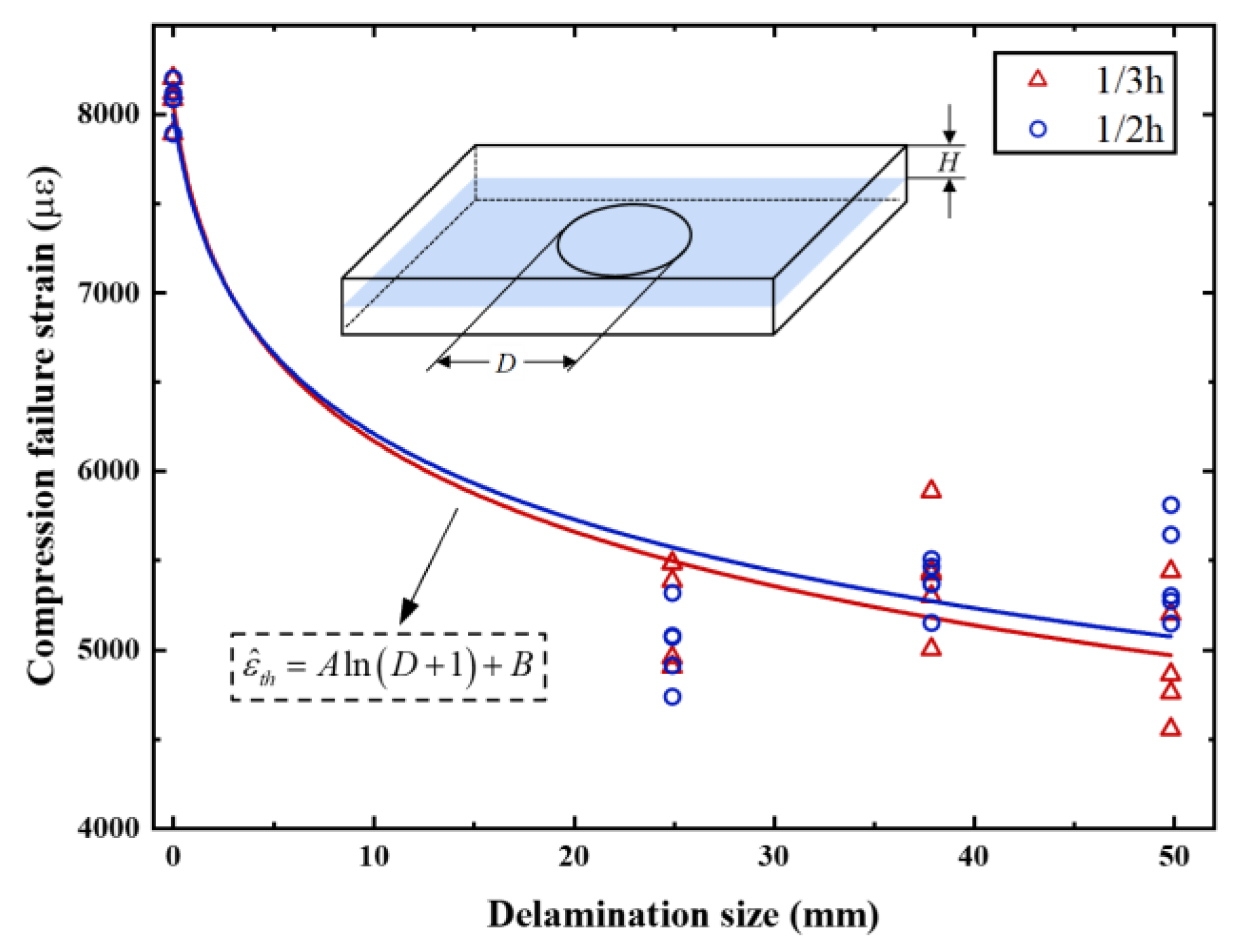
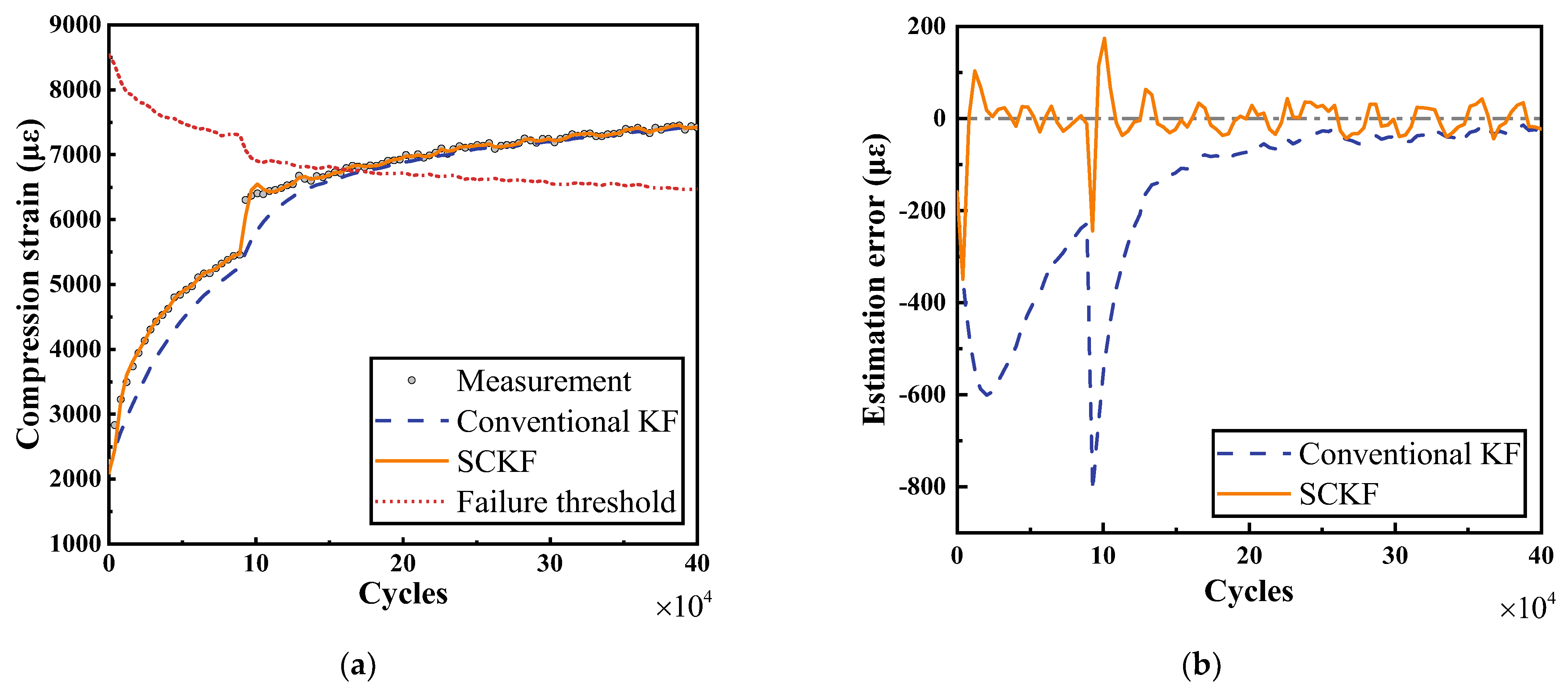
4.1. The Time-Varying Failure Threshold

An important premise for applying performance degradation data for RUL prediction is making an accurate definition of the structural failure. Generally, structural failure is considered to occur when the degradation value reaches the corresponding failure threshold. Therefore, for increasing degradation processes, a low failure threshold will make the predicted life lower than the true value, leading to inefficient use of the structure, and, conversely, resulting in a higher estimate than the true life, where the structural safety is not fully guaranteed. However, the currently used failure thresholds are usually set based on empirical domain knowledge, thus an experimental or theoretical basis is lacking for high prediction accuracy. Instead, we took into account an experiment-based failure threshold, which is related to the damage state of the composite laminates, providing a new solution to this problem.
The compression test results on composite laminates with delamination revealed that compression failure strain is highly dependent on the embedded delamination size, and failure strain largely reflects the compression carrying capacity of composite laminates [36]. The larger the size of the delamination deficiency inside the laminate, the lower the externally applied displacement required for the laminate to reach failure. Therefore, we took the compression failure strain as the failure threshold of the compression strain, which is associated with the delamination size.
According to the experimental results in [36], Figure 1 shows the variation in compression failure strain of composite laminates with delamination size. In this figure, as the delamination size increases, the compression failure strain quickly decreases, and the rate of the decrease gradually diminishes. As the delamination size increases from 0 to 25 mm, the compression failure strain decreases by more than 35%. However, when the delamination size is larger than 25 mm, there is no significant difference between the compression failure strains. In addition, it can be found that the delamination depth position has little impact on the compression failure strain for the results of h / 3 and h / 2 , which are quite close. From that, a logarithm prediction model was established as
ε t h = A ln ( D + 1 ) + B + ε
where ε t h is the compression failure strain, D is the delamination size, A and B are the regressive parameters, and ε is a random variable with zero expectation.
By comparing the compression failure strain with the actual compression strain of the laminates, the remaining life of composite structures can be further assessed. It is worth noting that the compression failure strain was derived from static test results, and the effect of fatigue cyclic loading was neglected. In other words, only the effect of delamination on the structural failure threshold was considered, while the effects of other types of deficiencies such as matrix cracking and matrix/fiber debonding were not taken into consideration.

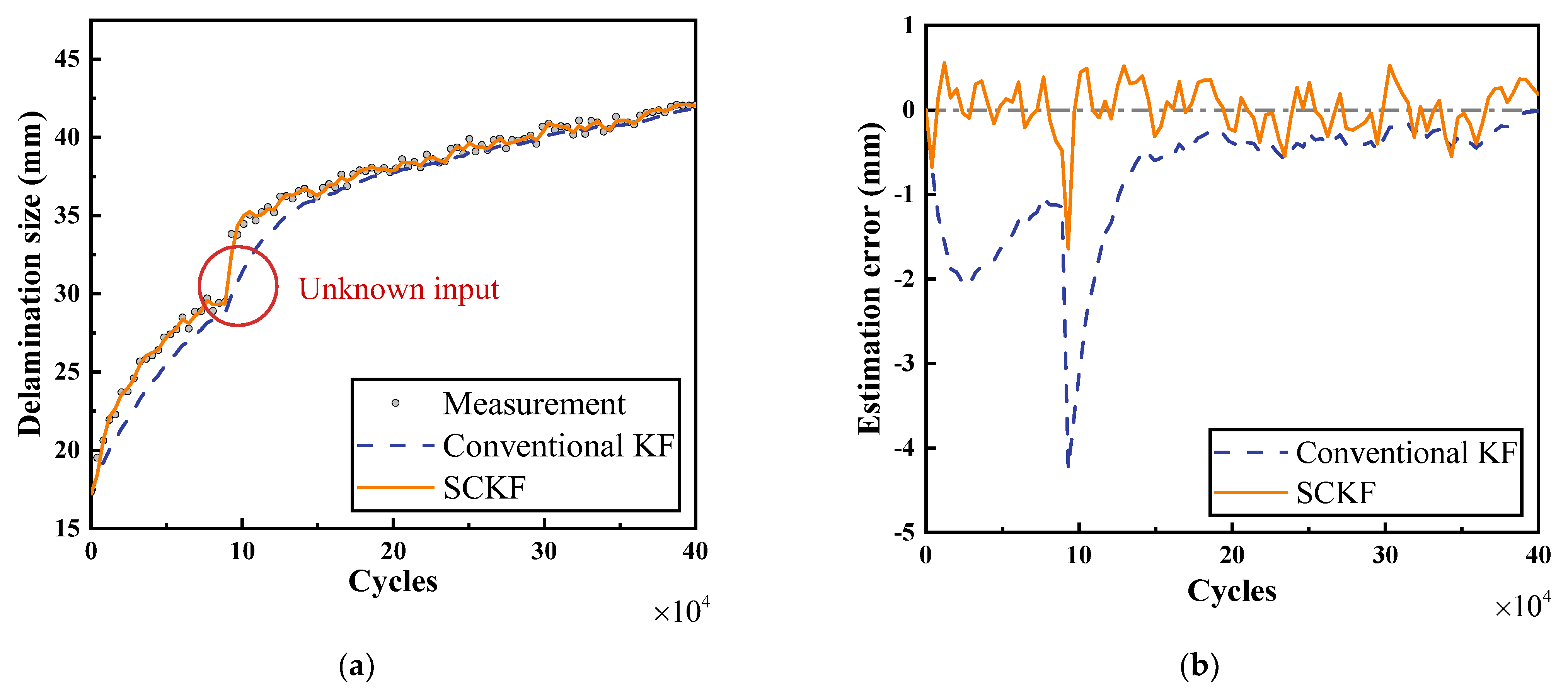
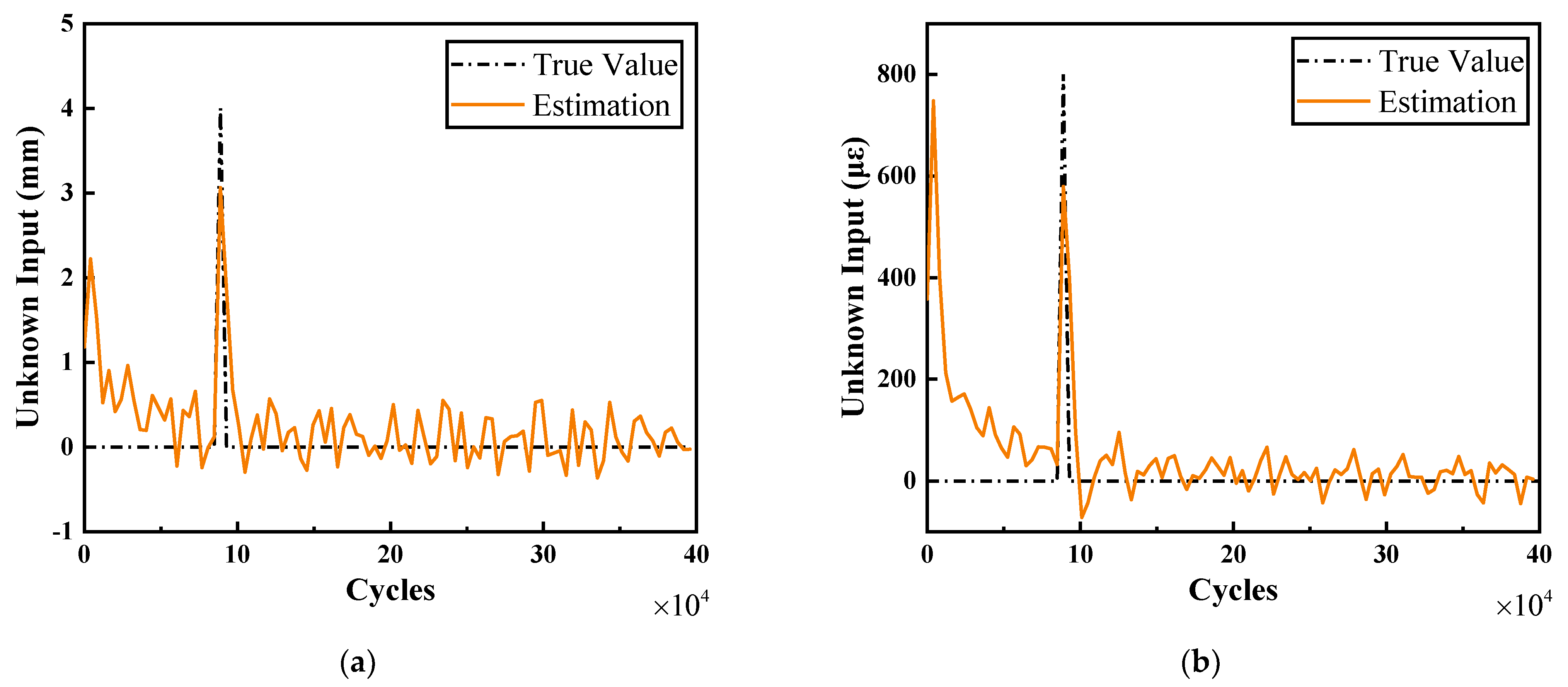
4.2. RUL Prediction of Composite Laminates with Delamination

The state equation used for SCKF is described as
y k = D k ε k λ D , k λ ε , k = 1 0 1 0 0 1 0 1 0 0 1 0 0 0 0 1 D k 1 ε k 1 λ D , k 1 λ ε , k 1 + b D , k + ω D b ε , k + ω ε ω λ D ω λ ε
where ω D , ω ε , ω λ D , and ω λ ε are four independent Gaussian white noises with covariance of Q .
The measurement equation includes direct observations of delamination size and compression strain,
z k = D k ε k + ν D ν ε
where ν D and ν ε are independent measurement noises with covariance matrix R .
Due to the lack of structural health condition monitoring data of composite laminates under fatigue loading, we employed a simulation example to illustrate the implementation of the proposed method. According to the description of fatigue delamination propagation in composite laminates in [20], it is assumed that the delamination first rapidly grows and then gradually tends to slow down with increased fatigue loading; that is, the delamination growth rate decreases with increasing delamination size. Moreover, the residual stiffness usually decreases with increasing load cycles and its degradation rate gradually declines, as can be seen in [20,21,37]. Because compression strain is inversely correlated with residual stiffness, the evolution path of compression strain can also be assumed. In addition, an abrupt increase of 4 mm in delamination size and a decrease of 800 με in compression strain were set at 100,000 cycles to simulate a foreign impact of the composite laminate during service. This is because the impact of foreign objects often causes a sudden increase in internal damage and a decrease in stiffness of composite laminates. In the simulation, the measurement z k was generated by adding zero-mean noise to the degradation path described above.
The SCKF and the traditional KF were separately applied to estimate the structural degradation, and their results are illustrated in Figure 2 and Figure 3. As can be seen from Figure 2a and Figure 3a, the SCKF could compensate for the unknown inputs in a short time. This is because the SCKF models the unknown input in the state equation and establishes both the connection between the unknown inputs of adjacent two-step filters and the connection between the unknown inputs and the state variables, as described in Equations (5), (9), and (10). However, because the unknown inputs are not considered, the conventional KF cannot identify the unknown inputs, and the influence of unknown inputs can only be partly reduced by measurement updates. Therefore, the estimation errors of SCKF were maintained around zero with less fluctuation, while there were larger estimation errors with conventional KF, as shown in Figure 2b and Figure 3b.
The estimation results of unknown inputs are shown in Figure 4. It can be found the SCKF was basically capable of tracking the unknown inputs, which provided a basis for accurate estimation of the system state.
In addition, the root mean square error of the estimation results was further calculated to compare the performance of the two filtering methods,
RMSE k = 1 n i = 1 n x ^ i , k x i , k 2
where n is the number of independent numerical simulations, x ^ i , k represents the estimated value of the system state at the k th point in the i th simulation, and x i , k is the true value. The average RMSE of 8000 simulations is shown in Table 2. It can be found that compared with the conventional KF, the average RMSE of the SCKF for delamination size and compression strain were reduced by 60.25% and 76.52%, respectively, indicating that the state estimations of the SCKF were closer to the true values, and the SCKF had a higher accuracy of state estimation.
Based on the estimation results of the structural degradation state and failure threshold shown in Figure 3a, the remaining life of composite laminates could be predicted, whose results are illustrated in Figure 5. With an increasing number of observed measurements, the predicted RUL curve gradually decreases and converges to the true RUL, and its 95% confidence interval gradually narrows. The final predicted service life was obtained as 153,900 cycles, which had a relative error of 4.76% compared with the real service life of 161,600 cycles. It is important to note that the true value of the RUL was obtained from the noise-free simulated data of delamination growth and compression evolution, whereas the prediction was carried out in a noisy environment; thus, this low relative error cannot validate the failure threshold used in this study.

5. Conclusions

This paper proposed a remaining life prediction method for composite laminates under unknown inputs and time-varying failure threshold conditions. First, a Wiener-process-based model was utilized to characterize the fatigue damage evolution of composite laminates, where an unknown input was involved. Then, an SCKF-based framework for state estimation was developed and implemented with a simulation example. In the simulation, a foreign impact was set to occur on the laminates under fatigue loading, and the results demonstrated that the SCKF could identify and estimate the unknown input quicker than the conventional Kalman filter, and the average RMSE of the SCKF for delamination size and compression strain was reduced by 60.25% and 76.52%, respectively. Finally, the compression failure strain was selected to be the failure threshold for predicting RUL, which was experimentally rather than empirically determined, and was associated with the delamination size.
However, the proposed method is only applicable to the constant-amplitude loading spectrum, and the failure threshold implemented must be further validated with fatigue tests. For further research, the life consumption may be introduced to predict the RUL of composites under variable-amplitude loading. The external environment condition has an impact on the performance of the composite material and the measurement of the sensors, which must be further explored.

Author Contributions

Conceptualization, J.G. and Y.Z.; methodology, J.G. and J.W.; software, J.G.; validation, J.G.; formal analysis, J.G. and J.W.; investigation, J.G. and Y.Z.; resources, J.G.; data curation, J.G.; writing—original draft preparation, J.G.; writing—review and editing, J.W. and Y.Z.; visualization, J.G.; supervision, Y.Z.; project administration, Y.Z.; funding acquisition, Y.Z. All authors have read and agreed to the published version of the manuscript.

Funding

This research was funded by the National Natural Science Foundation of China, grant number 52005159.

Institutional Review Board Statement

Not applicable.

Informed Consent Statement

Not applicable.

Data Availability Statement

Not applicable.

Conflicts of Interest

The authors declare no conflict of interest.

References

  1. Zhang, J.; Peng, L.; Zhao, L.; Fei, B. Fatigue Delamination Growth Rates and Thresholds of Composite Laminates under Mixed Mode Loading. Int. J. Fatigue 2012, 40, 7–15. [Google Scholar] [CrossRef]
  2. Gong, Y.; Li, W.; Liu, H.; Yuan, S.; Wu, Z.; Zhang, C. A Novel Understanding of the Normalized Fatigue Delamination Model for Composite Multidirectional Laminates. Compos. Struct. 2019, 229, 111395. [Google Scholar] [CrossRef]
  3. D’Amore, A.; Giorgio, M.; Grassia, L. Modeling the Residual Strength of Carbon Fiber Reinforced Composites Subjected to Cyclic Loading. Int. J. Fatigue 2015, 78, 31–37. [Google Scholar] [CrossRef]
  4. Wan, A.; Xiong, J.; Xu, Y. Fatigue Life Prediction of Woven Composite Laminates with Initial Delamination. Fatigue Fract. Eng. Mater. Struct. 2020, 43, 2130–2146. [Google Scholar] [CrossRef]
  5. Zong, J.; Yao, W. Fatigue life prediction of composite structures based on online stiffness monitoring. J. Reinf. Plast. Compos. 2017, 36, 1038–1057. [Google Scholar] [CrossRef]
  6. Gao, J.; Zhu, P.; Yuan, Y.; Wu, Z.; Xu, R. Strength and Stiffness Degradation Modeling and Fatigue Life Prediction of Composite Materials Based on a Unified Fatigue Damage Model. Eng. Fail. Anal. 2022, 137, 106290. [Google Scholar] [CrossRef]
  7. Dong, H.; Li, Z.; Wang, J.; Karihaloo, B.L. A New Fatigue Failure Theory for Multidirectional Fiber-Reinforced Composite Laminates with Arbitrary Stacking Sequence. Int. J. Fatigue 2016, 87, 294–300. [Google Scholar] [CrossRef]
  8. Lynch, J.P. A Summary Review of Wireless Sensors and Sensor Networks for Structural Health Monitoring. Shock Vib. Dig. 2006, 38, 91–128. [Google Scholar] [CrossRef] [Green Version]
  9. Farrar, C.R.; Worden, K. An Introduction to Structural Health Monitoring. Philos. Trans. R. Soc. Math. Phys. Eng. Sci. 2007, 365, 303–315. [Google Scholar] [CrossRef]
  10. Wu, Z.; Qing, X.P.; Chang, F.-K. Damage Detection for Composite Laminate Plates with A Distributed Hybrid PZT/FBG Sensor Network. J. Intell. Mater. Syst. Struct. 2009, 20, 1069–1077. [Google Scholar] [CrossRef]
  11. Da Silva, L.F.M.; Moreira, P.M.G.P.; Loureiro, A.L.D. Determination of the Strain Distribution in Adhesive Joints Using Fiber Bragg Grating (FBG). J. Adhes. Sci. Technol. 2014, 28, 1480–1499. [Google Scholar] [CrossRef] [Green Version]
  12. Grave, J.H.L.; Haheim, M.L.; Echtermeyer, A.T. Measuring Changing Strain Fields in Composites with Distributed Fiber-Optic Sensing Using the Optical Backscatter Reflectometer. Compos. Part B Eng. 2015, 74, 138–146. [Google Scholar] [CrossRef]
  13. Cantero-Chinchilla, S.; Malik, M.K.; Chronopoulos, D.; Chiachio, J. Bayesian Damage Localization and Identification Based on a Transient Wave Propagation Model for Composite Beam Structures. Compos. Struct. 2021, 267, 113849. [Google Scholar] [CrossRef]
  14. Khomenkd, A.; Karpenko, O.; Koricho, E.; Haq, M.; Cloud, G.L.; Udpa, L. Theory and Validation of Optical Transmission Scanning for Quantitative NDE of Impact Damage in GFRP Composites. Compos. Part B Eng. 2016, 107, 182–191. [Google Scholar] [CrossRef]
  15. Saeedifar, M.; Zarouchas, D. Damage Characterization of Laminated Composites Using Acoustic Emission: A Review. Compos. Part B Eng. 2020, 195, 108039. [Google Scholar] [CrossRef]
  16. Feng, T.; Bekas, D.; Aliabadi, M.H.F. Active Health Monitoring of Thick Composite Structures by Embedded and Surface-Mounted Piezo Diagnostic Layer. Sensors 2020, 20, 3410. [Google Scholar] [CrossRef]
  17. Andreades, C.; Fierro, G.P.M.; Meo, M. A Nonlinear Ultrasonic SHM Method for Impact Damage Localisation in Composite Panels Using a Sparse Array of Piezoelectric PZT Transducers. Ultrasonics 2020, 108, 106181. [Google Scholar] [CrossRef]
  18. Chalioris, C.E.; Kytinou, V.K.; Voutetaki, M.E.; Karayannis, C.G. Flexural Damage Diagnosis in Reinforced Concrete Beams Using a Wireless Admittance Monitoring System-Tests and Finite Element Analysis. Sensors 2021, 21, 679. [Google Scholar] [CrossRef]
  19. Peng, T.; Liu, Y.; Saxena, A.; Goebel, K. In-Situ Fatigue Life Prognosis for Composite Laminates Based on Stiffness Degradation. Compos. Struct. 2015, 132, 155–165. [Google Scholar] [CrossRef]
  20. Corbetta, M.; Sbarufatti, C.; Giglio, M.; Saxena, A.; Goebel, K. A Bayesian Framework for Fatigue Life Prediction of Composite Laminates under Co-Existing Matrix Cracks and Delamination. Compos. Struct. 2018, 187, 58–70. [Google Scholar] [CrossRef]
  21. Banerjee, P.; Palanisamy, R.P.; Udpa, L.; Haq, M.; Deng, Y. Prognosis of Fatigue Induced Stiffness Degradation in GFRPs Using Multi-Modal NDE Data. Compos. Struct. 2019, 229, 111424. [Google Scholar] [CrossRef]
  22. Liu, Y.; Mohanty, S.; Chattopadhyay, A. Condition Based Structural Health Monitoring and Prognosis of Composite Structures under Uniaxial and Biaxial Loading. J. Nondestruct. Eval. 2010, 29, 181–188. [Google Scholar] [CrossRef]
  23. Chiachío, J.; Chiachío, M.; Sankararaman, S.; Saxena, A.; Goebel, K. Condition-Based Prediction of Time-Dependent Reliability in Composites. Reliab. Eng. Syst. Saf. 2015, 142, 134–147. [Google Scholar] [CrossRef] [Green Version]
  24. Eleftheroglou, N.; Loutas, T. Fatigue Damage Diagnostics and Prognostics of Composites Utilizing Structural Health Monitoring Data and Stochastic Processes. Struct. Health Monit. 2016, 15, 473–488. [Google Scholar] [CrossRef]
  25. Loutas, T.; Eleftheroglou, N.; Zarouchas, D. A Data-Driven Probabilistic Framework towards the in-Situ Prognostics of Fatigue Life of Composites Based on Acoustic Emission Data. Compos. Struct. 2017, 161, 522–529. [Google Scholar] [CrossRef]
  26. Banerjee, P.; Karpenko, O.; Udpa, L.; Haq, M.; Deng, Y. Prediction of Impact-Damage Growth in GFRP Plates Using Particle Filtering Algorithm. Compos. Struct. 2018, 194, 527–536. [Google Scholar] [CrossRef]
  27. Pugalenthi, K.; Trung Duong, P.L.; Doh, J.; Hussain, S.; Jhon, M.H.; Raghavan, N. Online Prognosis of Bimodal Crack Evolution for Fatigue Life Prediction of Composite Laminates Using Particle Filters. Appl. Sci. 2021, 11, 6046. [Google Scholar] [CrossRef]
  28. Eleftheroglou, N.; Zarouchas, D.; Loutas, T.; Alderliesten, R.; Benedictus, R. Structural Health Monitoring Data Fusion for In-Situ Life Prognosis of Composite Structures. Reliab. Eng. Syst. Saf. 2018, 178, 40–54. [Google Scholar] [CrossRef] [Green Version]
  29. Cristiani, D.; Sbarufatti, C.; Giglio, M. Damage Diagnosis and Prognosis in Composite Double Cantilever Beam Coupons by Particle Filtering and Surrogate Modelling. Struct. Health Monit. 2021, 20, 1030–1050. [Google Scholar] [CrossRef]
  30. Yong Lee, I.; Doh Roh, H.; Park, Y.-B. Prediction Method for Propagating Crack Length of Carbon-Fiber-Based Composite Double Cantilever Beam Using Its Electromechanical Behavior and Particle Filter. Compos. Struct. 2022, 279, 114650. [Google Scholar] [CrossRef]
  31. Si, X.-S.; Wang, W.; Hu, C.-H.; Chen, M.-Y.; Zhou, D.-H. A Wiener-Process-Based Degradation Model with a Recursive Filter Algorithm for Remaining Useful Life Estimation. Mech. Syst. Signal Process. 2013, 35, 219–237. [Google Scholar] [CrossRef]
  32. Ye, Z.-S.; Chen, N. The Inverse Gaussian Process as a Degradation Model. Technometrics 2014, 56, 302–311. [Google Scholar] [CrossRef]
  33. Lin, Y.-H.; Ding, Z.-Q. An Integrated Degradation Modeling Framework Considering Model Uncertainty and Calibration. Mech. Syst. Signal Process. 2022, 166, 108389. [Google Scholar] [CrossRef]
  34. Xiao, M.; Zhang, Y.; Wang, Z.; Fu, H. An Adaptive Three-Stage Extended Kalman Filter for Nonlinear Discrete-Time System in Presence of Unknown Inputs. ISA Trans. 2018, 75, 101–117. [Google Scholar] [CrossRef]
  35. Simon, D. Optimal State Estimation: Kalman, H Infinity, and Nonlinear Approaches; John Wiley & Sons: Hoboken, NJ, USA, 2006; ISBN 0-470-04533-7. [Google Scholar]
  36. Guo, J.; Zhang, Y.; Chen, K. Algorithm for Compression Design Allowable Determination of Composite Laminates with Initial Delaminations. Machines 2021, 9, 307. [Google Scholar] [CrossRef]
  37. Huang, J.; Pastor, M.L.; Garnier, C.; Gong, X.J. A New Model for Fatigue Life Prediction Based on Infrared Thermography and Degradation Process for CFRP Composite Laminates. Int. J. Fatigue 2019, 120, 87–95. [Google Scholar] [CrossRef]
Figure 1. The compression failure strain as structural failure threshold.
Machines 10 01185 g001
Figure 2. Estimation results of delamination size and their errors. (a) Estimation results of D k . (b) Estimation error of D k .
Machines 10 01185 g002
Figure 3. Estimation results of compression strain and their errors. (a) Estimation results of ε k and failure threshold. (b) Estimation error of ε k .
Machines 10 01185 g003
Figure 4. Estimation results of SCKF for unknown inputs. (a) Estimation results of unknown input of D k . (b) Estimation results of unknown input of ε k .
Machines 10 01185 g004
Figure 5. RUL prediction of composite laminates considering unknown inputs.
Machines 10 01185 g005
Table 1. Summary of real-time prediction methods for RUL of composites (2010–2022).
Specimen TypeDamage VariablesSensors/Sensing TechnologiesReferences
Composite beam with notchDamage indexStrain gaugeLiu et al. [22] (2010)
Composite plate with notchMicrocrack density,
delamination area, stiffness
PZT, strain gauge, X-rayChiachío et al. [23] (2015)
Open-hole composite plateResidual stiffnessPZTPeng et al. [19] (2015)
Open-hole composite plateAE featureAEEleftheroglou et al. [24] (2016),
Loutas et al. [25] (2017)
Open-hole composite plateMatrix crack density,
delamination area, stiffness
X-ray, strain gaugeCorbetta et al. [20] (2018)
Impacted composite plateDelamination areaOTSBanerjee et al. [26] (2018),
Pugalenthi et al. [27] (2021)
Open-hole composite plateFeature valueAE, digital image correlation (DIC)Eleftheroglou et al. [28] (2018)
Open-hole composite plateResidual stiffnessOTS, GWBanerjee et al. [21] (2019)
Composite double cantilever beam (DCB)Delamination lengthFiber Bragg grating strain
sensor
Cristiani et al. [29] (2020)
Composite DCBCrack lengthDigital multimeterLee et al. [30] (2022)
Table 2. Comparison of RMSE between SCKF and conventional KF.
Filtering Method Average RMSE
Delamination Size (mm)Compression Strain (με)
KF1.3005279.6375
SCKF0.517065.6601
Publisher’s Note: MDPI stays neutral with regard to jurisdictional claims in published maps and institutional affiliations.

